Bringing Modeling to the Masses: A Web Based System to Predict Potential Species Distributions

Abstract

Predicting current and potential species distributions and abundance is critical for managing invasive species, preserving threatened and endangered species, and conserving native species and habitats. Accurate predictive models are needed at local, regional, and national scales to guide field surveys, improve monitoring, and set priorities for conservation and restoration. Modeling capabilities, however, are often limited by access to software and environmental data required for predictions. To address these needs, we built a comprehensive web-based system that: (1) maintains a large database of field data; (2) provides access to field data and a wealth of environmental data; (3) accesses values in rasters representing environmental characteristics; (4) runs statistical spatial models; and (5) creates maps that predict the potential species distribution. The system is available online at www.niiss.org, and provides web-based tools for stakeholders to create potential species distribution models and maps under current and future climate scenarios.

1. Introduction

Predicting species current and potential distributions is critical to the effective management of invasive species [1], conservation of threatened and endangered species [2,3,4], and protection of native species and habitats [5]. Accurate predictive models can guide field surveys [6,7], define monitoring priorities [8], and help direct conservation and restoration efforts at local, regional, and national scales [9].

Over the past few decades, statistical and technical capabilities have progressed to a level where we now have a variety of techniques for predicting the potential distribution of a given species [10,11,12,13]. These techniques use field observations of a species (i.e., presence-absence data or presence-only data) as a dependent variable, while independent or predictive variables represent environmental conditions (e.g., elevation, minimum temperature, mean monthly precipitation). Methods such as Maximum Entropy modeling [14] and the Genetic Algorithm for Rule-set Prediction [15] require only presence locations of a species as the dependent variable. Model algorithms are designed to analyze the statistical relationships between the dependent variable and independent variables and create geospatial representations of where a species is likely to occur and where it is likely absent. To date, these tools and methods have only been available to a small audience of researchers with the time and resources to bring together the data, the software, and acquire the knowledge to run the software required to create models.

With today’s computer hardware, computer software, and the Internet, we can bring modeling capabilities to a much wider audience, and strengthening the capacity of resource managers and citizen scientists while providing learning opportunities for K-12 teachers, students and young scientists. Advances in computer hardware and software have made it possible to setup and maintain computer servers that store large geospatial datasets, perform complex analyses on demand, and provide access to the data and analysis capabilities through a website [16]. Commercial and open source software can be assembled with custom programming into a system that is robust, secure, and reliable. The Internet provides access to web pages from anywhere in the world through the World-Wide-Web. Through web scripting we can provide access to analysis capabilities in a secure yet easy to use interface.

There are many websites that allow users access to species occurrences records [17,18]. There are also several systems that are beginning to provide predicted surfaces of potential species distributions. The Global Biodiversity Information Facility includes the ability to create world-wide maps of potential species distributions based on the openModeler software package [19]. Different spatial model algorithms are available for use with openModeller, generally producing world-wide maps at fairly coarse resolution, but with limited means to assess model uncertainty at various scales and levels of resolution [20]. LifeMapper is another website which includes models from BIOLIM and GARP [21]. What is missing is a system that provides the ability for any web user to collect field data, integrate it with other data, run distribution models against environmental layers, create predictive distribution maps, and do so at a variety of spatial scales. Our objective was to create such a system and make it available over the World-Wide-Web. The target audience for this system includes managers, citizen scientists, and students who do not have the expertise, resources, or time to develop models that are available to research scientists immersed in modeling.

2. Methods

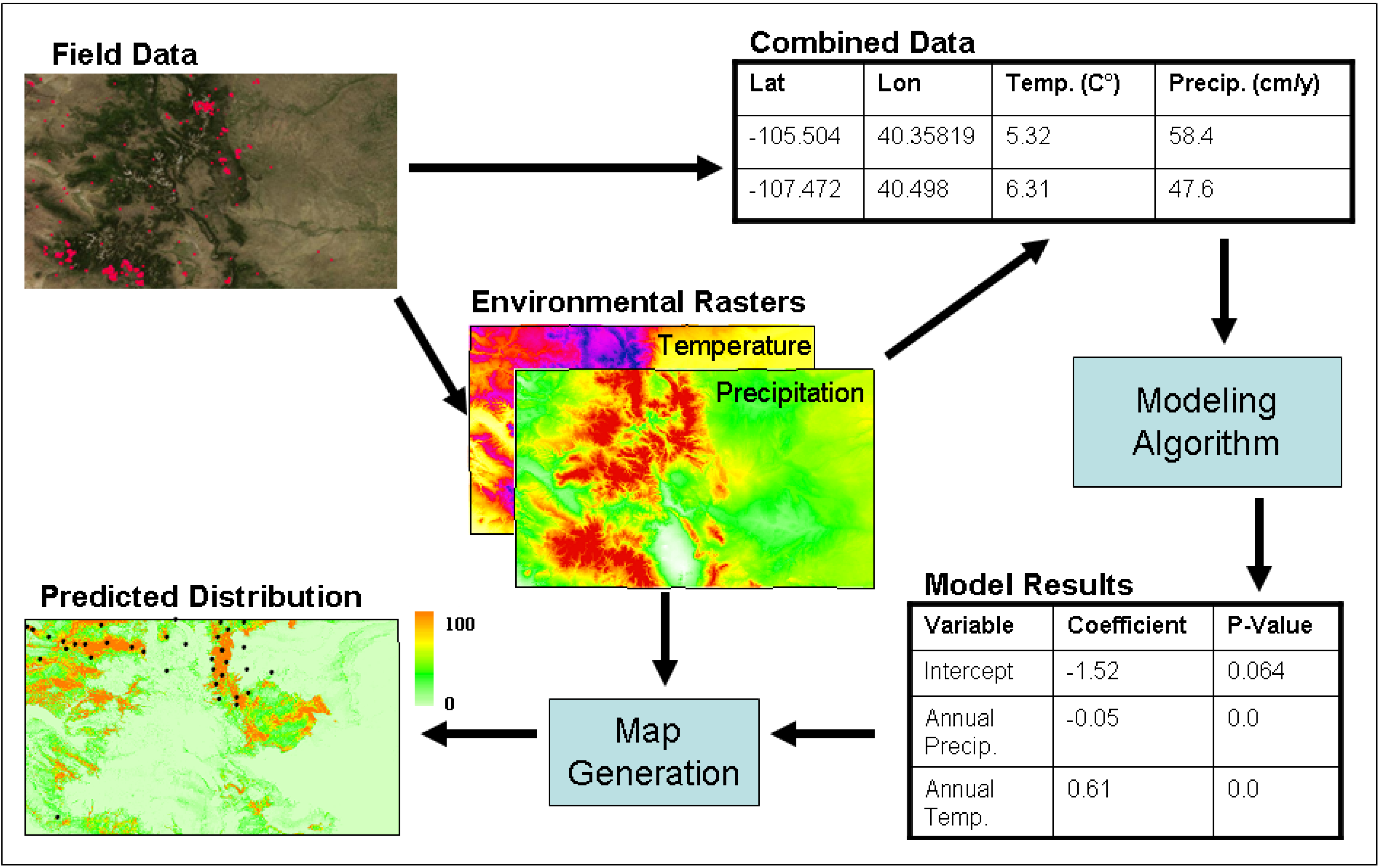
Most spatial modeling techniques share a common process to create a spatial model and a predicted surface. This process includes: obtaining coordinates for species occurrences, extracting environmental predictor values for each coordinate based on environmental layers, running a model algorithm to produce model results, and creating a map of the predicted potential distribution for the species from model results (Figure 1). The requirements for creating predictive species distribution models on the Web include: (1) a database of field data representing species occurrences; (2) a repository of environmental data in raster format; (3) the ability to execute and store results from a variety of statistical models; and (4) the ability to create and display maps based on the results of statistical models. Here, we describe how predictive modeling was added to our existing web system, the International Biological Information System (IBIS) which includes the Global Organism Detection and Monitoring (GODM) system for mapping suitable habitats of invasive species in real time [16].

Figure 1. Overview of the process for creating a potential distribution map for the invasive plant Dalmatian Toadflax (Linaria dalmatica) in the state of Colorado in the United States of America. The final map is in percent probability that the area is suitable for Dalmatian Toadflax.

Figure 1. Overview of the process for creating a potential distribution map for the invasive plant Dalmatian Toadflax (Linaria dalmatica) in the state of Colorado in the United States of America. The final map is in percent probability that the area is suitable for Dalmatian Toadflax.

2.1. Maintaining a Large Database of Field Data

Since field data can come in many formats, the system provides multiple methods to contribute data. Users can enter data into online forms, collect data with personal digital assistants (PDAs), or upload spreadsheet-type data. Online data entry forms can also be created. These forms include information such as location, date, and taxonomy information, and can be customized to include organism attributes such as height and percent cover. The forms can be downloaded to a PDA and then the collected data can be uploaded directly to the website from the PDA through web services.

Field data can also be augmented by data that are ‘harvested’ from other sources [22]. The availability of data for predicting potential species distributions is growing as web systems provide the ability to download data [23]. Our system can capitalize on this additional data though web services and by allowing the upload of spreadsheets directly to the system [16,24].

There are a variety of options for the projection and datum in modeling species distributions. Since model outputs placed on the Web using transparent tiles provided in the GoogleMaps projection can meet user performance expectations [25], and because most modeling algorithms do not require equal-distant or equal-area spatial data, field data and environmental layers were projected into the GoogleMaps projection which always uses the World Geodetic System 1984 (WGS 84) as it’s datum. After the user selects an area for study and a species to model, the system extracts the appropriate field data and saves it in a tab-delimited text file.

2.2. Providing Access to Environmental Data

Environmental data are typically provided in a raster image file where each picture element (pixel) represents a rectangular area on the earth. The value of each pixel then represents an environmental measurement at that location. These files are then organized into “layers” of data which may contain multiple rasters to cover a large spatial extent. Common environmental variables include data from weather stations, field measurements, and remotely sensed data. Variables derived from weather station data include a wide variety of climatic variables such as minimum or maximum annual temperature, number of growing degree days, annual precipitation, humidity, and the amount of sunlight available at each location, typically provided as Photosynthetically Active Radiation. While these measurements are typically acquired from individual weather stations, they often are provided as raster files with continuous cover for a large geographic region such as Daymet [26].

The GODM system was created to allow immediate access to field data and to create potential species distribution maps at different extents including local, national, and global scales and at multiple spatial resolutions. This capability required a very flexible, robust, and high-performance system for integrating field data with many environmental data layers. A relational database was used to create a hierarchical structure for the environmental data. The structure encodes all of the available files by location, resolution, date, and type of information they contain. The system then selects the correct data based on the required resolution, area being viewed, and whether the data are intended for viewing or analysis.

We loaded a large number of default climate layers for the United States into the system from the BioClim dataset [27]. Since Maxent supports creating predicted future distributions of species based on future climate predictions, we added the option of running potential distributions in the year 2050. We used uncompressed Tagged Image File Format (TIFF) files to allow access to the original data for analysis. This design allows Web users to select a single “layer” with environmental information such as minimum temperature; the system can then select exactly which layers are needed for analysis. Each time a model is run, the environmental layers are cropped to the area of interest and then saved in the file format desired by the modeling algorithm.

2.3. Running Statistical Models

Originally, the GODM system included a variety of models including linear regression, logistic regression, and regression trees. Since the bulk of available data only contain presence points, and Maxent requires only presence points, Maxent became the preferred approach.

One of the benefits of placing statistical models on the Web is the opportunity to change the user interface of the modeling software from one that is typically challenging for most users (even research scientists) to one that is much easier to use. The process of executing a model includes: (1) converting the data to a format supported by the statistical package; (2) dynamically creating a script that will execute the desired models and includes user selected and computed parameters for the model; (3) calling the package through a “command-line” interface; (4) monitoring progress of the model; and (5) displaying the model results. These steps can be hidden from the user behind “web pages” that provide an easier to use and overall simpler interface. By necessity some features of the modeling package are hidden to simplify creating models for novice users with links to the available modeling engines for users to access as they desire more advanced features.

Since the user can select any number of layers and the amount of time to create models with multiple layers can be several hours, the models are run under a “job controller,” which limits the number of jobs running at any one time to two and notifies the user when the job is completed through an automatically generated email. This approach both ensures that the server is not overloaded with jobs and that each job is completed sequentially. Unfortunately, Maxent does not output progress information so a standard “progress bar” appears but does not move while the model is running.

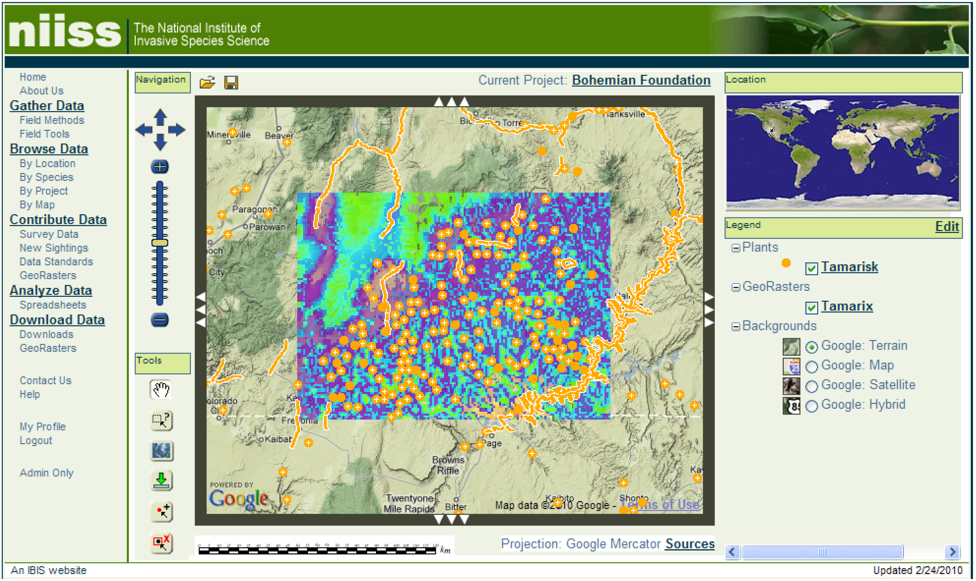
Figure 2. A screen capture of the mapping portion of the NIISS website with the Habitat Suitability Modeler button highlighted.

Figure 2. A screen capture of the mapping portion of the NIISS website with the Habitat Suitability Modeler button highlighted.

After the user has completed a model, they are given the opportunity to create a map of their predicted model or review model results. Creating a map is a “one-button” approach, where the user simply clicks a button and the model results are used to create a predicted surface that matches the extent of the field data they selected. Currently the resolution of the images is limited to a 1-km² grid to match the large quantity of environmental layers that are available at this resolution. Since GODM includes a complete mapping system, the user can then view their predicted surface overlaid on top of the original field data they used to generate the model along with other desired data (Figure 2). The predicted surfaces are saved and can be downloaded by the user to their local computer for further analysis if desired.

3. Results

The system is available at the website for the National Institute of Invasive Species Science (www.niiss.org), one of many IBIS websites (the full list of sites is available at www.ibis.colostate.edu). Users can upload data to the system or use existing data. To create a predicted surface using Maxent include: (1) select the “Make a Map” tool in the mapping web page; (2) select the species to model; and (3) select the environmental layers to use in the model. After clicking the final ‘Submit’ button, a progress bar will appear followed by the initial MaxEnt model output. From here the user can examine detailed modeling results, create a version of their model to view on the map, or return to the map to try a different area or species. This simple Web process reduces the time to create models from weeks to minutes compared to prior workflows (e.g., collect and integrate field data, gather environmental data, and install and learn modeling software).

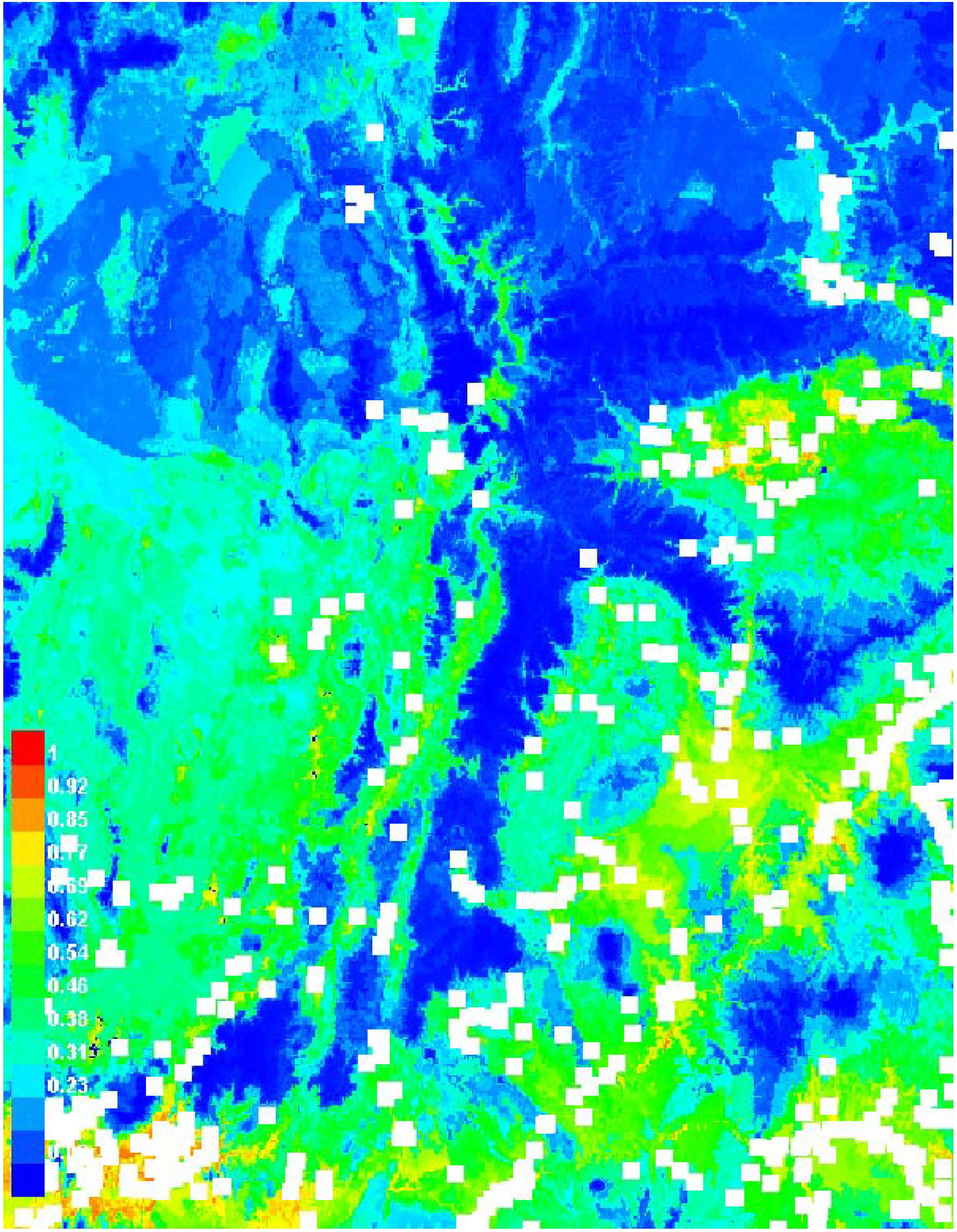
Figure 3. A screen capture of the mapping portion of the NIISS website with a model of the potential distribution of members of the genus Tamarix within the Grand Staircase-Escalante National Monument, Utah.

Figure 3. A screen capture of the mapping portion of the NIISS website with a model of the potential distribution of members of the genus Tamarix within the Grand Staircase-Escalante National Monument, Utah.

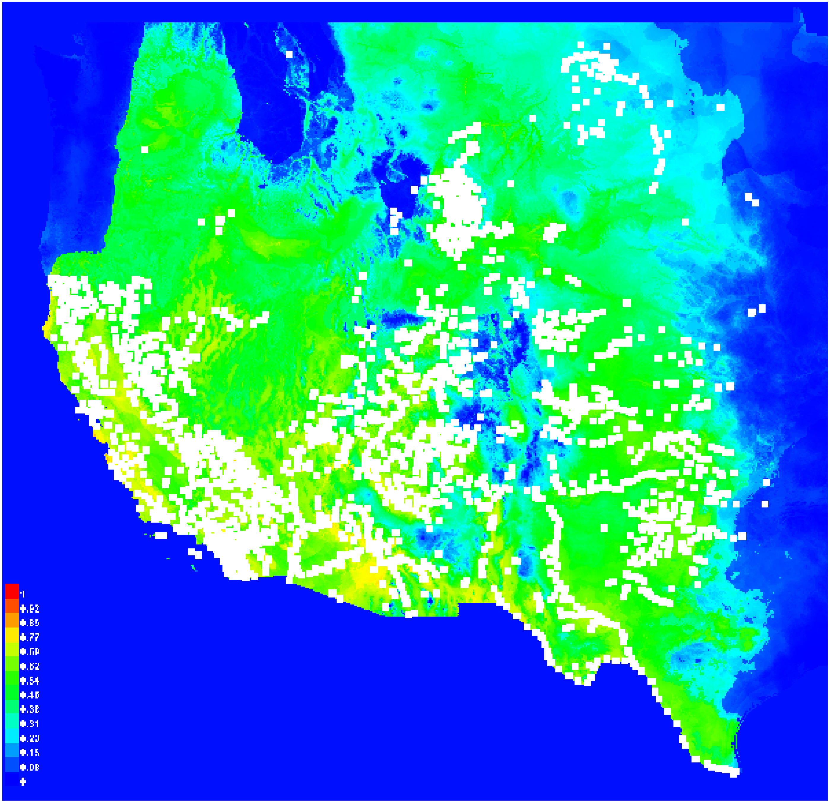
Figure 4. The model output for Tamarix within the state of Utah.

Figure 4. The model output for Tamarix within the state of Utah.

As an example, we used the system to model the invasive plant Tamarix sp. distributions at three different scales: (1) the Grand Staircase–Escalante National Monument (Figure 3); (2) the state of Utah (Figure 4); and (3) the western United States (Figure 5). First, each model was run with all available environmental layers, and then run again using the five environmental layers that contributed most to the model (Table 1). It is interesting to note that different environmental layers were important at different scales. Information for the layers is available within the modeling pages of the web site, while the full results of these models are available on the IBIS web site at http://tinyurl.com/28zcs44.

The selection of species and area was based on the availability of data in the system at the time of analysis. The system currently contains a large number of surveys for the invasive species Tamarix and national-scale environmental layers typically used for modeling terrestrial plants [6,7]. There are also data for a variety of other invasive species. If the system does not contain field data required to run a model, users can add additional data through the web site before running a model. In the future, users may be able to add additional environmental layers for their own area of interest.

Figure 5. The model output for Tamarix in the western United States.

Figure 5. The model output for Tamarix in the western United States.

Table 1. The Area Under the Curve (AUC), and top five predictor layers for each of the three scales of models, and the percent that each environmental variable contributed to the model.

Region Modeled/Environmental Layer	Contribution (%)
1. Grand Staircase – Escalante National Monument (AUC = 0.77)
1.1 Annual Mean Temperature	29.3
1.2 Distance To Water	22.2
1.3 Min Temperature of Coldest Month	18.6
1.4 Mean Temperature of Coldest Quarter	16.0
1.5 Mean Diurnal Range	14.0
2. State of Utah (AUC = 0.84)
2.1 Number of Growing Days	43.6
2.2 Max Temperature of Warmest Month	24.9
2.3 Mean Diurnal Range	21.2
2.4 Enhanced Vegetation Index (EVI) Range	83.0
2.5 Temperature Annual Range	2.0
3. Western United States (AUC = 0.86)
3.1 Isothermality	54.3
3.2 Frequency of Precipitation	14.9
3.3 Precipitation of Driest Month	12.0
3.4 Maximum Temperature of Warmest Month	9.4
3.5 Precipitation of Warmest Quarter	9.3

Table 1. The Area Under the Curve (AUC), and top five predictor layers for each of the three scales of models, and the percent that each environmental variable contributed to the model.

Region Modeled/Environmental Layer	Contribution (%)
1. Grand Staircase – Escalante National Monument (AUC = 0.77)
1.1 Annual Mean Temperature	29.3
1.2 Distance To Water	22.2
1.3 Min Temperature of Coldest Month	18.6
1.4 Mean Temperature of Coldest Quarter	16.0
1.5 Mean Diurnal Range	14.0
2. State of Utah (AUC = 0.84)
2.1 Number of Growing Days	43.6
2.2 Max Temperature of Warmest Month	24.9
2.3 Mean Diurnal Range	21.2
2.4 Enhanced Vegetation Index (EVI) Range	83.0
2.5 Temperature Annual Range	2.0
3. Western United States (AUC = 0.86)
3.1 Isothermality	54.3
3.2 Frequency of Precipitation	14.9
3.3 Precipitation of Driest Month	12.0
3.4 Maximum Temperature of Warmest Month	9.4
3.5 Precipitation of Warmest Quarter	9.3

4. Conclusions

The type of technology described herein was not designed to replace existing data collection and analysis techniques, but rather facilitate applications and education in geospatial sciences for a wider audience. Our results showed that the system is capable of multi-scale modeling applying key environmental variables regularly used for predicting species distributions. Just as important, we provide a user-friendly interface allowing new users to run models within a single day, and in some cases, the duration of a class period. This is far less time than it would take to install and master Geographic Information Systems and MaxEnt software, gather and format environmental datasets, and run a model.

Currently the system only creates a single raster for the area bounded by the selected occurrence data and the system does not expose all of the options available for the MaxEnt modeling engine. The environmental layers are also currently limited to the continental United States. To extend this system, we plan to include consistent global environmental layers, add additional modeling techniques, provide more options for each modeling technique, and improve hardware performance. The ability to add data from directly from existing on-line databases, such as the Global Biodiversity Information Facility, is also being implemented through web services. A protocol is being developed specifically for accessing data for invasive species as part of the Global Invasive Species Information Network [28]. Future objectives also include developing training and educational materials to increase the user’s understanding of modeling concepts, proper applications and, equally important, their limitations. We remain excited about the prospects these technologies offer to stakeholders, and hope our efforts provide new opportunities for resource management, environmental stewardship, education for all ages, and public participation