Dynamic Lognormal Shadowing Framework for the Performance Evaluation of Next Generation Cellular Systems

Abstract

Performance evaluation tools for wireless cellular systems are very important for the establishment and testing of future internet applications. As the complexity of wireless networks keeps growing, wireless connectivity becomes the most critical requirement in a variety of applications (considered also complex and unfavorable from propagation point of view environments and paradigms). Nowadays, with the upcoming 5G cellular networks the development of realistic and more accurate channel model frameworks has become more important since new frequency bands are used and new architectures are employed. Large scale fading known also as shadowing, refers to the variations of the received signal mainly caused by obstructions that significantly affect the available signal power at a receiver’s position. Although the variability of shadowing is considered mostly spatial for a given propagation environment, moving obstructions may significantly impact the received signal’s strength, especially in dense environments, inducing thus a temporal variability even for the fixed users. In this paper, we present the case of lognormal shadowing, a novel engineering model based on stochastic differential equations that models not only the spatial correlation structure of shadowing but also its temporal dynamics. Based on the proposed spatio-temporal shadowing field we present a computationally efficient model for the dynamics of shadowing experienced by stationary or mobile users. We also present new analytical results for the average outage duration and hand-offs based on multi-dimensional level crossings. Numerical results are also presented for the validation of the model and some important conclusions are drawn.

1. Introduction

Wireless communication systems have offered outstanding achievements and opportunities for applications and services in information and communication technologies. In the upcoming 5G era, the future cellular networks should be envisioned to support efficient and flexible resource management and provide customized services to meet the service-specific high performance requirements in a variety of use cases. New higher frequency bands are also allocated for employment in future cellular networks and in order to support the new challenging demands of the users that generally need more bandwidth. The propagation channel plays one of the most crucial roles in order to provide reliable communications, high availability systems and also determine efficiently the system dimensioning (number of antennas, relays, base stations, gateways etc.). The future cellular architectures are becoming more complex and the performance of different types of links in multiuser, multi-cells, small cells, and relaying scenarios that are changing topology very frequently should be evaluated. Moreover, the upcoming 5G communication systems are planned to accommodate various diverse services and satisfying their stringent performance requirements in terms of connectivity, mobility, reliability, latency, peak data rate, and coverage will impose unprecedented challenges to 5G network design and performance optimization. This will be achieved with the 5G terminology of networks slicing. To this end, the link adaptation considering the spatial-temporal time varying propagation channel in the various cells that provide different services will remain one of the most important problems for the optimum design of the future satellite systems, including also their synergetic architectures. Regarding the current status of the propagation research, there are numerous measurement campaigns in various environments and different frequencies and also many theoretical approaches for statistical channel models [1,2,3,4,5,6]. Nevertheless in experimental campaigns have not studied the temporal variation of the large scale fading that is due to the movement of the local environment scatterers, especially for millimeter wave frequencies.

Wireless channel models consist of an indispensable tool for the efficient design and testing of modern wireless communication systems. The emerging need for higher data payloads demands more sophisticated exploitation of the channel’s capabilities, which in turn imposes further requirements for the development and application of more advanced channel models. In this paper we focus on large scale fading or shadowing.

This kind of fading, that is mainly caused by obstructions, has been commonly accepted to be modeled as a lognormal random variable for outdoor [7] and indoor environments [8]. Whereas shadowing is a purely spatial phenomenon for a specific configuration of the propagation environment, temporal variability is induced mainly by the user’s mobility but also by moving obstructions. The impact of shadowing caused by moving obstructions, even for fixed locations, may have an important role in the system’s performance, especially in densely populated environments. In this context, shadowing can be considered as a spatio-temporal process, i.e., a random field evolving in time. Moreover, the impact of shadowing correlation is considered nowadays as a key parameter to account for in order to obtain more realistic channel model frameworks. Taking into account the correlation structure of the shadowing field impels shadowing modeling one step further towards reality, as shadowing correlation significantly affects handover behavior, interference power and the performance of diversity schemes [9].

Various existing models in the literature exploit the spatial correlation structure of the shadowing field, without taking into account the temporal variability [10,11,12,13], while others that include the temporal evolution consider it solely a result of user’s mobility, by transforming the spatial correlation to temporal, without really addressing the temporal evolution of the field, mainly caused by obstruction movement in the vicinity of the receiver [14,15,16]. This is especially important in indoor environments [17], when line of sight (LOS) is disturbed, as several studies indicate, see [18,19] and the references therein. Similar results, although less intense, are expected for distributed indoor-outdoor and/or densely populated urban networks [18]. However in these models, shadowing correlation and cross-correlation for different locations and base stations are not taken into account.

Whereas autocorrelation of shadowing refers to the case of one base transmitter, cross-correlation refers to the correlated shadowing of signals from different base stations. This statistical behavior of differently originated signals is of great importance for the design of cellular wireless networks, interference studies, handover algorithms, cooperative diversity schemes, etc. The correlation phenomenon is present in outdoor [20], as well as in indoor environments [21,22,23]. Moreover even links without a common node, if closely located, exhibit shadowing correlation [23,24]. In [25] a stochastic differential equation (SDE) is introduced for shadowing dynamic modeling, able to capture the random attenuation variations with respect to time, but without considering shadowing cross-correlations from different base stations, either.

Moreover some publications from the application of correlated shadowing phenomena in relaying architectures and cooperative networks are [26,27,28,29,30,31] and on stochastic differential equations are [32,33].

Up to now, in the literature there are not analytical dynamic statistical channel models for the large scale fading that could be used for the evaluation of complex wireless network architectures. Therefore there is a strong motivation to develop a theoretical model with parameters that can be adopted to experimental measurements.

In this paper, a novel dynamic shadowing model (channel model framework) is proposed, able to deal with the temporal evolution of the propagation environment and also incorporate the spatial correlation structure, by considering any type of correlation exhibited by different radio links, including auto-correlation and cross-correlation. The model assumes the lognormal distribution for shadowing fading, incorporating all important statistical parameters, as validated from experimental studies. While being consistent with existing shadowing literature and published results, it captures every important aspect of shadowing modeling in a single framework. It is based on a system of stochastic differential equations (SDEs), and its solid mathematical framework permits the calculation of important statistical parameters, while keeping complexity and computational cost to accepted levels. The model can be used for the effective design and simulation of fixed and mobile wireless systems.

In this paper there novel analytical results are also presented concerning average outage durations (AOD), level crossing rates (LCR) and hand-offs, based on the proposed probabilistic structure of shadowing and the method of multi-dimensional level crossings.

The strengths of the proposed approach are the employment and the usage of many theoretical models in order to develop a consolidated space–time dynamic model for large scale fading. The components of the model are well accepted and have been proved theoretically. The weakness of the approach is that it needs experimental verification. To the authors’ best knowledge there are not specific measurements in the literature to validate the proposed modeling. For future experimental campaigns, it is important to design a specific experiment in order to quantify to and study the temporal variability of the large scale fading.

The remainder of the paper is structured as follows: Section 2 introduces the model and addresses several aspects of its application with many mathematical details. In Section 3, numerical results of the proposed model are presented and some significant conclusions are drawn.

2. Dynamic Lognormal Shadowing Framework

2.1. Random Field of Shadowing

Shadowing refers to the random variations of the received signal power around a mean value that is noticed when a user is located at a given distance from a base station. This variation is mainly caused because of different objects located in the radio-path and not taken into account by path gain models that are used for the calculation of the mean power based only on distance. Thus, these fluctuations are taken into account in a statistical manner and the received signal to noise ratio $SN{R}_R$ for a specific location is expressed in logarithmic scale as:

$$SN{R}_R=SN{R}_T-\overline{PL}(d)+X\hspace{1em}(\mathrm{dB})$$

(1)

where $SN{R}_T$ is the transmitted signal to noise ratio and $\overline{PL}(d)$ is the mean propagation loss, as calculated by an appropriate path loss model dependent only on the distance d between the base station and the receiver. The term X in (1) is the shadowing component, a random variable (r.v.) location specific, commonly accepted to be zero mean Gaussian [7].

Denoting by ${\gamma }_R$ the received signal to noise ratio in linear scale, then from (1) it is evident that it is a lognormal r.v. with a probability density function (pdf) given by:

$$p(\gamma )=\frac{\xi }{\gamma \sqrt{2\pi }\sigma }{e}^{-\frac{(10\log \gamma -\mu )}{2{\sigma }^2}}$$

(2)

where $\xi =10/\ln 10$ is a normalization constant and $\mu$ (dB) and $\sigma$ (dB) are the mean and the standard deviation of $10\log {\gamma }_R$ respectively. The standard deviation σ of $10\log {\gamma }_R$ is actually that of X, whereas the mean μ expressed in terms of the median ${\gamma }_m$ of ${\gamma }_R$ and the transmission characteristics is given by:

$$\mu =\ln ({\gamma }_m)=\ln {\gamma }_T-\frac{1}{\xi }\overline{PL}$$

(3)

where ${\gamma }_T$ is the transmitted signal to noise in linear scale.

In (1) and what follows we assume that any multipath losses have been filtered out and we focus next on the shadowing r. v. X. This is modeled for a given base station placement as a random field $X(\mathbf{x})$ with correlated values in different locations, what is known as serial correlation or autocorrelation of shadowing. Though being traditionally modeled as a time-invariant spatial process, it is actually a spatio-temporal process $S(\mathbf{x},t)$. The temporal evolution is caused by variabilities in the propagation environment caused by moving obstructions. As wireless networking becomes a critical requirement even in complex and unfavorable environments, a novel dynamic shadowing model is presented here able to deal with the temporal evolution of shadowing. In this section we present the proposed model mostly informally through the covariance structure in order to explain the motivation and to show the similarity to well accepted models in the literature. The covariance function permits not only the second order description of the shadowing random field, but its complete characterization, as it is a Gaussian random field.

A commonly accepted autocorrelation model for shadowing is a simple exponential characterized by the shadowing correlation distance $r_c$ [34].

$$\rho ({\mathbf{x}}_1,{\mathbf{x}}_2)=e^{-\frac{|{\mathbf{x}}_2-{\mathbf{x}}_1|}{r_c}}$$

(4)

The variance of shadowing is referred to as location variability $\sigma$ and depends on frequency and the propagation environment (urban, suburban, indoors, etc.). It is usually assumed common for all locations belonging to the same general category of environment. Thus the spatial covariance of shadowing is described as:

$$C({\mathbf{x}}_1,{\mathbf{x}}_2)=e^{-\frac{|{\mathbf{x}}_2-{\mathbf{x}}_1|}{r_c}}{\sigma }^2$$

(5)

It is a common practice when the user is moving this spatial variability to be translated to a temporal variability scaled according to mobile’s speed. This is a standard scenario for measuring the spatial variability, however careful data averaging is used to exclude the effects of multipath fading. In this case (5) is transformed to:

$$C(t_1,t_2)=e^{-\frac{|\mathbf{v}\Vert t_2-t_1|}{r_c}}{\sigma }^2=e^{-a|t_2-t_1|}{\sigma }^2$$

(6)

where $a=-\frac{\left|\mathbf{v}\right|}{r_c}$, introducing thus the temporal autocorrelation as:

$$\rho (t_1,t_2)=e^{-a|t_2-t_1|}$$

(7)

However, movement is a relative phenomenon and the influence of moving obstacles to shadowing for fixed users can also be taken into account in a similar manner. We may thus attribute movement to obstacles and consider a fixed user. We introduce for a fixed point $\mathbf{X}$ the temporal autocorrelation of (7), which assuming a location specific variance $\sigma (\mathbf{x})$ and dynamic parameter $a(\mathbf{x})$ results in the following temporal autocovariance:

$$C_{\mathbf{x}}(t_1,t_2)=e^{-a(\mathbf{x})|t_2-t_1|}\sigma {(\mathbf{x})}^2$$

(8)

In order to express the temporal variability along with the spatial for two fixed locations ${\mathbf{x}}_1,{\mathbf{x}}_2$ in two different time instants $t_1,t_2$ we notice that the choice of the exponential temporal autocorrelation for each location implies that the shadowing process is Gaussian and Markov. Thus, without loss of generality, assuming $t_1<t_2$, we can express the shadowing r.v. $S({\mathbf{x}}_2,t_2)$ in terms of $S({\mathbf{x}}_2,t_1)$ as:

$$S({\mathbf{x}}_2,t_2)=e^{-a({\mathbf{x}}_2)|t_2-t_1|}S({\mathbf{x}}_2,t_1)+\sigma ({\mathbf{x}}_2)\sqrt{1-e^{-2a({\mathbf{x}}_2)|t_2-t_1|}}N$$

(9)

where $N$ is a standard normal r.v. independent of the shadowing parameters. By using (9) we find that the covariance function of the shadowing random field $S(\mathbf{x},t)$ is expressed as

$$C({\mathbf{x}}_1,t_1,{\mathbf{x}}_2,t_2)=e^{-a({\mathbf{x}}_2)|t_2-t_1|}\rho ({\mathbf{x}}_1,t_1,{\mathbf{x}}_2,t_1)\sigma ({\mathbf{x}}_1)\sigma ({\mathbf{x}}_2)$$

(10)

where stationarity is assumed. The correlation coefficient can be chosen as:

$$\rho ({\mathbf{x}}_1,t_1,{\mathbf{x}}_2,t_1)=e^{-\frac{|{\mathbf{x}}_2-{\mathbf{x}}_1|}{r_c}}$$

(11)

and in this case (10) describes the temporal evolution of auto-correlation of shadowing for a fixed user. A similar reasoning has been used in [35] for the case of cross-correlation of shadowing affecting a mobile user. With the selection of an appropriate correlation coefficient, the covariance function (10) can be easily modified to include cross-correlation of shadowing and any correlation exhibited by adjacent links.

We assume $m$ base stations and the vector shadowing random field $\mathbf{S}(\mathbf{x},t)=[S_1(\mathbf{x},t),\dots ,S_m(\mathbf{x},t)]$, where $S_i(\mathbf{x},t),\hspace{0.17em}i=1,\dots ,m$ is the shadowing process affecting a station located at $\mathbf{x}$ receiving the signal from base station $i,\hspace{0.17em}i=1,\dots ,m$. The vector random field is completely described by the cross-covariances:

$$C_{ij}({\mathbf{x}}_1,t_1,{\mathbf{x}}_2,t_2)={\rho }_{ij}({\mathbf{x}}_1,t_1,{\mathbf{x}}_2,t_2){\sigma }_i({\mathbf{x}}_1){\sigma }_j({\mathbf{x}}_2)$$

(12)

where ${\rho }_{ij}({\mathbf{x}}_1,t_1,{\mathbf{x}}_2,t_2)$ is the correlation coefficient between the shadowing processes at points ${\mathbf{x}}_1,{\mathbf{x}}_2$ for the time instants $t_1,t_2$ respectively and for the signals from base stations $i,j$. It may be chosen in a general setting to express autocorrelation, cross-correlation of shadowing, as well as correlation between adjacent links without a common node. The model proposed here assumes the exponential temporal correlation model:

$${\rho }_{ij}({\mathbf{x}}_1,t_1,{\mathbf{x}}_2,t_2)=e^{-a({\mathbf{x}}_2)|t_2-t_1|}{\rho }_{ij}({\mathbf{x}}_1,t_1,{\mathbf{x}}_2,t_1)$$

(13)

Stationarity is also assumed by considering ${\rho }_{ij}({\mathbf{x}}_1,t_1,{\mathbf{x}}_2,t_1)$ independent of time. Except for these prerequisites any consistent correlation model may be used. A reasonable choice reflecting the commonly accepted correlation dependencies is given in [36] by:

$${\rho }_{ij}({\mathbf{x}}_1,t_1,{\mathbf{x}}_2,t_1)=e^{-\frac{|{\mathbf{x}}_2-{\mathbf{x}}_1|}{r_c}}g({\theta }_{x_1}^i-{\theta }_{x_2}^j)h(d_{x_1}^i-d_{x_2}^j)$$

(14)

where ${\theta }_{x_i}^j$ is the direction of point ${\mathbf{x}}_i$ from base station $j$ relative to some reference direction and $d_{x_i}^j$ is the distance of point ${\mathbf{x}}_i$ from base station $j$. The functions $g,\hspace{0.17em}h$ are chosen in a way to satisfy positive definiteness according to [36]. A detailed account for issues concerning the feasibility of selected correlation models can be found in [9]. In [24] another model based on an underlying spatial loss field is proposed in terms of a line integral across links, permitting the shadowing correlation calculation, even for links without a common node. In any case of a feasible spatial correlation model chosen, the proposed model induces an exponential temporal correlation as in (13). As shadowing is considered a Gaussian random field [36] an appropriate selection of a feasible correlation model gives a positive definite covariance matrix for any selection of space and/or time points.

Before proceeding in the next section to the formulation of the proposed dynamic model it should be noted that the location variabilities appearing in (5)–(12) depict the fact that shadowing is being dealt with in a statistical manner as path gain models do not take into account the exact propagation environment. This kind of modeling is described as non-site specific. This is one of the main advantages of the proposed dynamic channel model framework. The location variability represents the statistical spread of shadowing over the space–time points used for averaging. In case that detailed studies for a specific environment have been carried out by use of other techniques, like ray tracing, then it is only the influence of moving obstacles that has to be studied in a statistical manner and only temporal averaging is used. We refer to these cases as site-specific. Then $\sigma$ describes the variability that these moving objects can cause to the received power for each specific location and the value of $\sigma$ is expected to be lower, than in the case that coarse path gain models are used and space averaging is used. Even in cases where detailed measurements have not been carried out, but some specific propagation conditions may be recognized, then this can impact the value of the location variability through the introduction of an appropriate bias, like in [37,38].

Now based on the temporal exponential model and the implicit Markov assumption the model proposed here can be formulated in the next section in terms of a system of stochastic differential equations (SDEs). Such a formulation permits a phenomenological description of the shadowing field with an additional solid mathematical background providing analytic calculations and straight-forward simulation methods.

2.2. Dynamic Model

We consider the received SNR from $m$ base stations, at $k$ locations of interest. We denote by ${\gamma }_i(t),\hspace{0.17em}i=1,\dots ,n=mk$ (The notations $\gamma (t)$ or ${\gamma }_t$ is used interchangeably for the time dependence), the received SNR in linear scale, i.e., every index corresponds to a specific location for a specific base station. According to (1) expressed in terms of SNR (dB) the SNR in linear scale ${\gamma }_i$ can be modeled as a lognormal r. v. for each time instant. Its long-term statistical parameters are ${\sigma }_i$ and $\ln \left({\gamma }_{m_i}\right)$. We are introducing the following multi-dimensional stochastic model. We assume that the resulting shadowing vector process $\mathbf{X}(t)=[X_1(t),\dots ,X_n(t)]$ after applying the nonlinear transformation:

$$X_i(t)=\xi \ln \left({\gamma }_i(t)/{\gamma }_{m_i}\right),\hspace{1em}1\le i\le n$$

(15)

to each component process ${\gamma }_i(t)$, is a solution to a linear n-dimensional SDE of Ornstein–Uhlenbeck type [39]:

$$d{\mathbf{X}}_t=\mathbf{A}·{\mathbf{X}}_{t}dt+\mathbf{B}·d{\mathbf{W}}_t,\hspace{0.17em}{\mathbf{X}}_0={\mathbf{x}}_0$$

(16)

where $\mathbf{A}$ is the diagonal matrix $\mathbf{A}={[a_{ij}]}_{1\le i,j\le n}$ with elements:

$$a_{ij}=-a_i·{\delta }_{ij}$$

(17)

${\delta }_{ij}$ is the Kronecker delta function and $a_i,\hspace{0.17em}1\le i\le n$ are the dynamic parameters of shadowing, in principle different for each link and $\mathbf{X}(0)={\mathbf{x}}_0$ is the initial condition of the stochastic differential equation. The solution to the n-dimensional SDE (16) is straightforward and is given [39]:

$${\mathbf{X}}_t=e^{t·\mathbf{A}}·{\mathbf{X}}_0+e^{t·\mathbf{A}}·{\displaystyle \underset{0}{\overset{t}{\int }}{e}^{-s·\mathbf{A}}·\mathbf{B}·d{\mathbf{W}}_s}$$

(18)

where

$$e^{t·\mathbf{A}}={\displaystyle \sum _{n=0}^{\infty }\frac{t^n}{n!}{\mathbf{A}}^n}$$

(19)

Now due to the fact that the matrix $\mathbf{A}$ is diagonal (see (17)) it can be easily verified that

$${\left[{\mathrm{e}}^{t·\mathbf{A}}\right]}_{ij}=e^{-a_i·t}{\delta }_{ij}$$

(20)

The solution stochastic process ${\mathbf{X}}_t$ as given in (18) is a Gaussian process if ${\mathbf{X}}_0$ follows an n-variate normal distribution, including the degenerate case. The mean vector of ${\mathbf{X}}_t$, ${\mathbf{M}}_{\mathbf{X}}(t)$ is given by:

$${\mathbf{M}}_{\mathbf{X}}(t)=e^{t·\mathbf{A}}·{\mathbf{M}}_{\mathbf{X}}(0)$$

(21)

The covariance matrix ${\mathbf{C}}_{\mathbf{X}}(t)$ of the vector process ${\mathbf{X}}_t$ for each time instant $t$ is given [39]:

$${\mathbf{C}}_{\mathbf{X}}(t)=e^{t·\mathbf{A}}\left[{\mathbf{C}}_{\mathbf{X}}(0)+{\displaystyle \underset{0}{\overset{t}{\int }}{e}^{-s·\mathbf{A}}\mathbf{B}{\mathbf{B}}^T{e}^{-s·{\mathbf{A}}^T}ds}\right]e^{t·{\mathbf{A}}^T}$$

(22)

which is the solution to the following linear differential equation

$$\stackrel{•}{{\mathbf{C}}_{\mathbf{X}}}\left(t\right)=\mathbf{A}{\mathbf{C}}_{\mathbf{X}}(t)+{\mathbf{C}}_{\mathbf{X}}(t){\mathbf{A}}^T+\mathbf{B}{\mathbf{B}}^T$$

(23)

The matrix $\mathbf{A}$ has by definition all of its eigenvalues real and negative (equal to $-a_i$), so the convergence of the following integral is assured.

$${\mathbf{C}}_{\mathbf{X}}={\displaystyle \underset{0}{\overset{\infty }{\int }}{e}^{s·\mathbf{A}}\mathbf{B}{\mathbf{B}}^T{e}^{s·{\mathbf{A}}^T}ds}$$

(24)

It is easy to verify that if ${\mathbf{C}}_{\mathbf{X}}(0)={\mathbf{C}}_{\mathbf{X}}$ then ${\mathbf{C}}_{\mathbf{X}}(t)={\mathbf{C}}_{\mathbf{X}}$ is a solution to (23). This means that a stationary solution of (16) exists and in this case for (23) we are leading to the following algebraic matrix equation:

$$\mathbf{A}{\mathbf{C}}_{\mathbf{X}}+{\mathbf{C}}_{\mathbf{X}}{\mathbf{A}}^T=-\mathbf{B}{\mathbf{B}}^T$$

(25)

This equation forms the physical basis of the model. The stationary covariance matrix ${\mathbf{C}}_{\mathbf{X}}$ of ${\mathbf{X}}_t$ is equal to the covariance matrix of the shadowing process $\mathbf{S}(t)$. Thus, existing models for the shadowing process $\mathbf{S}(t)$ permit the derivation of the covariance matrix ${\mathbf{C}}_X$ of ${\mathbf{X}}_t$. Then, equation (25) can be used for the determination of the transformation matrix $\mathbf{B}$, that is required for the dynamic modeling of the process ${\mathbf{X}}_t$ in (16), given the matrix $\mathbf{A}$ and the stationary covariance matrix ${\mathbf{C}}_{\mathbf{X}}$.

If we denote:

$$\mathbf{G}=\mathbf{B}{\mathbf{B}}^T$$

(26)

then from (25) we can determine that $\mathbf{G}$ is given by

$${\left[G\right]}_{ij}=\left(a_i+a_j\right){[C_X]}_{ij}$$

(27)

The matrix C_X as a covariance matrix is real and symmetric and from (27) the same is true also for $\mathbf{G}$. The decomposition of $\mathbf{G}$ as the product $\mathbf{B}{\mathbf{B}}^T$ is straightforward and can be realized via Cholesky decomposition.

By use of the solution process (18) a straight-forward calculation based on the properties of the stochastic integral leads to the cross-covariance for two time instants $t_1<t_2$

$${\mathbf{C}}_{\mathbf{X}}(t_1,t_2)={\mathbf{C}}_{\mathbf{X}}{e}^{(t_2-t_1)·{\mathbf{A}}^T}$$

(28)

in direct relation to (13).

The model as formulated corresponds to the case of a fixed wireless system and captures the temporal variability of shadowing due to obstacle movement. Of great interest though is the case of mobile wireless systems. We consider the case of $m$ base stations and $l$ mobile users moving along the trajectories ${\mathbf{r}}_j(t)=(x_j(t),y_j(t)),\hspace{1em}j=1\dots l$. By discretizing each trajectory in $k_l$ points, separated by a distance corresponding to the distance scale of the shadowing process, we result in $n=m{\displaystyle \sum _l{k}_l}$ links. The model may be used now for these successive locations providing the temporal evolution of the shadowing experienced by the mobile users. The stationary covariance matrix contains the covariances of any pair of locations for the corresponding signals of any pair of base stations. By adding more locations we may include the trajectories of other mobiles too. However, such an implementation provides more than we need, as the process models the temporal evolution for each point of the trajectories, i.e., for every time instant we get $n=m{\displaystyle \sum _l{k}_l}$ shadowing values and we actually need $ml$.

By using (12)–(14) and the fact that ${\mathbf{x}}_2={\mathbf{x}}_1+\mathbf{v}(t_2-t_1)$, where $\mathbf{v}$ is the velocity vector of the mobile, we see that for a distance covered, such that the shadowing process may be considered locally stationary, the covariance of the shadowing experienced by a mobile user is described as:

$$C_{ij}(t_1,t_2)=e^{-a^{\prime }(\mathbf{x})|t_2-t_1|}g(\Delta \theta )h(\Delta d){\sigma }_i(\mathbf{x}){\sigma }_j(\mathbf{x})$$

(29)

where $a^{\prime }(\mathbf{x})=a(\mathbf{x})+\left|\mathbf{v}\right|/r_c$. This approximation may be considered valid as long as the movements are not of large scale and a stationary covariance matrix can approximate the shadowing correlations and cross-correlations, irrespective of the users mobility [37]. In this case the correlations and cross-correlations have to be calculated for a representative separation angle and distance while the dynamic parameters account also for user’s mobility.

Here we have to note, that the proposed model is based on the multi-dimensional SDE in equation (16) with the appropriate diffusion and drift coefficients. The SDE is not directly related to motion, but provides the necessary spatial and temporal variability through the corresponding covariance matrices and the rest parameters. The covariance matrix that has been assumed has been selected as well accepted and proved in the related literature concerning the spatial variability of shadowing. The concept of the mean speed of variability has been presented to induce the temporal variability. Consequently, it is not an equation of motion, and even not a Brownian motion. It is a SDE of Ornstein–Uhlenbeck type that describes the spatio-temporal statistical behavior of the modeled process.

2.3. Transition Probabilities

The process ${\mathbf{X}}_t$ as a solution to (18) is a Gaussian Markov process. The transition probability densities $p\left(\mathbf{x},t|\mathbf{y},s\right)$ are defined by:

$$P[\mathbf{x}<\mathbf{X}(t)\le \mathbf{x}+d\mathbf{x}|\mathbf{X}(s)=\mathbf{y}]=p(\mathbf{x},t|\mathbf{y},s)d\mathbf{x}$$

(30)

These can be derived by using the SDE solution and the properties of the stochastic integral or by solving the corresponding Fokker Planck Equation (FPE):

$${\partial }_{t}p(\mathbf{x},t|\mathbf{y},s)={\displaystyle \sum _i{\partial }_{x_i}\left[{\beta }_i{x}_{i}p(\mathbf{x},t|\mathbf{y},s)\right]}+\frac{1}{2}{\displaystyle \sum _{i,j}{\partial }_{x_i}{\partial }_{x_j}\left[G_{ij}p(\mathbf{x},t|\mathbf{y},s)\right]}.$$

(31)

Using the assumption of stationarity we have:

$$p(\mathbf{x},t|\mathbf{y},s)=p(\mathbf{x},t-s|\mathbf{y},0)$$

(32)

The expression of $p(\mathbf{x},t|\mathbf{y},s)$ is given by:

$$\begin{array}{c}p(\mathbf{x},t|\mathbf{y},s)=\frac{1}{\sqrt{{(2\pi )}^n\Delta }}\exp (K)\\ K=-\frac{1}{2}(\mathbf{x}-e^{(t-s)\mathbf{B}}·\mathbf{y}){\mathbf{C}}_{\mathbf{X}}^{-1}(t){(\mathbf{x}-e^{(t-s)\mathbf{B}}·\mathbf{y})}^T\end{array}$$

(33)

where $\Delta$ is the determinant of the covariance matrix ${\mathbf{C}}_{\mathbf{X}}(t)$ and ${\mathbf{C}}_{\mathbf{X}}^{-1}(t)$ is the inverse matrix assuming that it exists.

2.4. Fade Durations and Level Crossings

Of great importance to several aspects of wireless communications is the average outage or fade duration (AOD). AOD is a second order statistical property, which significantly affects packet length, channel coding schemes, length interleaver, etc. The dynamic model proposed here permits the calculation of AOD in a multidimensional setting by considering correlated shadowing and without the adoption of asymptotic results of level crossings as in [40].

The shadowing process of (18) is a vector stochastic process of Ornstein–Uhlenbeck type, i.e., a Gaussian and Markov process. It is a well-known fact already from the one dimensional case that the power carried by the high frequencies of such a process is so large that the AOD is zero and the average level crossing rate (LCR) is non-finite [41]. However the inductances and capacitances always present in the circuits used in radio engineering act to smooth the process [42], so analysis of fade durations may be done through appropriate filtering of the process (18). Similar approaches can be found in [21] for a general Markov process, and in [16,24,43] for the shadowing process.

The filtering approach finds a very strong reasoning based on the time scale of the physical process of shadowing. As shadowing refers to the local mean of the received signal power, this is calculated by measuring and averaging the power received over a spatial distance of 20–30 wavelengths in order to filter out the multipath fading [44]. The shadowing then experiences slow variations over distances of tens of wavelengths due to the presence of obstructions depending on their relative size. Translating to time scale by considering the effect of movement this gives rise to a coarser time scale of shadowing and an upper frequency limit of the shadowing process. However the limits are not strict, especially in dense environments like in indoor propagation channels, where the large and small scale phenomena tend to get mixed. Thus, averaging for finding the local mean by filtering out the multipath effect has the drawback that the resultant shadowing process is unable to reflect shadowing variations inside the averaging window [45]. We nevertheless assume through the whole study that the multipath effect has been eliminated, an assumption common in the shadowing literature. We also do not confine ourselves to a specific filtering method as in [16,24], where moving averages (temporal or local) have been considered. Instead, we consider any appropriate linear filtering. However, filtering has a major impact on second order statistics and the selection of the filter characteristics must correspond to the specific analysis scenario.

Now as filtering is a linear operation and the shadowing process is a Gaussian process, the same is true for the smoothed process, thus permitting the use of well-known facts for LCR and AOD of Gaussian processes. By use of the generalized Rice method for vector stochastic processes [46], we can calculate the out-crossing rate $v^{+}$ of a limit surface $\partial S$ bounding a domain $D$ in the space of values of the filtered process ${\mathbf{Z}}_t$ as

$$v^{+}={\displaystyle \underset{\partial S}{\int }\left\{{\displaystyle \underset{0}{\overset{\infty }{\int }}{\dot{z}}_n}{f}_{\mathbf{Z}{\dot{Z}}_n}(\mathbf{z},{\dot{z}}_n)d{\dot{z}}_n\right\}}d\mathbf{z}$$

(34)

where ${\dot{z}}_n={\mathbf{n}}^T(\mathbf{z})·\dot{z}$ is the normal velocity of vector process ${\mathbf{Z}}_t$ at the limit surface $\partial S$ and $f_{\mathbf{z}{\dot{Z}}_n}(\mathbf{z},{\dot{z}}_n)$ is the joint probability density function (PDF). As ${\mathbf{Z}}_t$ is a Gaussian vector process, its derivatives are independent of the process simplifying the expressions for the joint PDF.

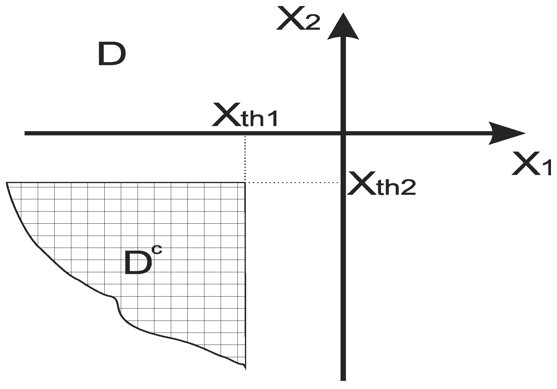
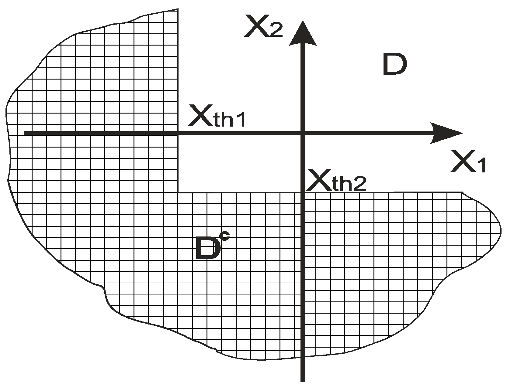
For any practical application of interest in wireless communications as in diversity schemes, multi-hop networks etc., a domain can be identified inside of which the values of the vector process permit the network operation, whereas out-crossings of this domain correspond to transitions to outage periods. For example for the case of selection combining (SC) in a dual diversity scheme the shaded area in Figure 1 corresponds to outage, whereas inside the domain D operation is assured. The values $X_{th1},X_{th2}$ correspond to threshold values below which the receiver cannot decode reliably. In Figure 2 the corresponding outage and operation domains are shown for the case of a regenerative dual-hop link.

The AOD is expressed in terms of the out-crossing rate as:

$$d=\frac{P({\mathbf{Z}}_t\in D^c)}{v^{+}}$$

(35)

where $D^c$ is the complement of $D$.

The study of LCR through an appropriately filtered process also gives insight to another aspect of the proposed model in relation to other approaches of the shadowing modeling by human shadowing. In [18,19] the shadowing effect is modeled by a finite-state Markov chain, where transition probabilities are derived. The shadowing event length is modeled as exponentially distributed and the appearance of obstacles as Poisson distributed. The model presented here may be considered also consistent with this approach, as it is well known that the level crossing of a high level of a Gaussian process is approximated by the Poisson distribution. The calculation of multi-dimensional LCR can be found in Appendix A.

Another application of the multi-dimensional LCR proposed here is the calculation of the average times per meter traveled that a moving mobile must switch base stations in order to always be served by the base station with the least path loss. As stated in [10] this is in fact, the basis for any good hand-off algorithm and can serve as a benchmark for comparison and evaluation of practical algorithms. The essential difference here with [16] is the novel application of multidimensional level crossings and the flexibility of dealing with any kind of filtering of the initial Markov process, instead only considering moving averages.

3. Numerical Results and Discussion

In this section we apply the proposed dynamic shadowing model to two practical and modern scenario scenarios of wireless systems. The first one refers to a dual-hop wireless system and the second one to a mobile station receiving signals from two base stations. There are also many practical scenarios that can be applied, such as interference, hand over, cooperative diversity, multiple antennas transmission and reception.

The system under consideration is supposed to operate according the specified requirements, when the received $SN{R}_R$ is greater than a threshold value $SN{R}_{TH}$, $SN{R}_R\ge SN{R}_{TH}$, or in linear scale ${\gamma }_R\ge {\gamma }_{TH}$. The threshold value depends on the type of modulation and the type of the supported application. This requirement may be translated in terms of the transformed process $X$ of (15), as:

$$X\ge SN{R}_{TH}-(SN{R}_T-\overline{PL}).$$

(36)

If we define the fade margin $FM$ as:

$$FM=SN{R}_T-\overline{PL}$$

(37)

and we assume for simplicity that $SN{R}_{TH}=0$ dB, by simply adding the threshold value to the propagation losses, then the requirement for operation is transformed to

$$X\ge -FM.$$

(38)

In order not to refer to specific equipment characteristics we present the results in relation to the fade margin. When the receiver is moving, assuming local stationarity over the characteristic area for shadowing, we present the results as a function of distance covered for a specific trajectory, assuming an initial fade margin value and referring to the specific large scale fading model used for the subsequent variation of the fade margin as the mobile moves.

As stated also previously, to the authors’ best knowledge there are no specific measurements in the literature to validate the proposed approach. The future experimental campaigns should be designed in order to capture the dynamic temporal variability of the large scale fading e.g., in a crowded local environment for various sites and for different frequency bands.

3.1. Dual-Hop

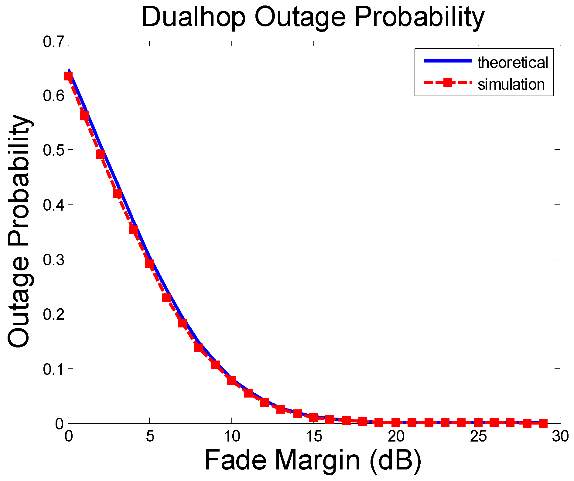
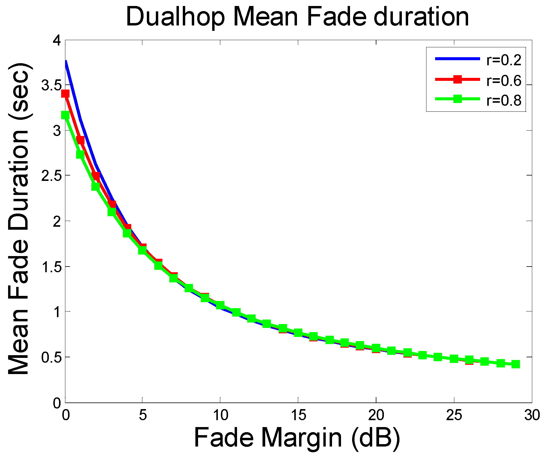
The first application refers to a regenerative dual-hop relay link, part of a wireless mesh network (WMN). The nodes are denoted $A,B$ and $C$ located at a distance $d$ apart. The system is located in a densely populated indoor environment, as a mall or an airport. The average speed of moving objects is considered to be that of pedestrians, as 1.5 m/s, whereas the shadowing decorrelation distance has been chosen 3 m, a value typical for indoor environments. The links are considered balanced, i.e., with the same fade margin.

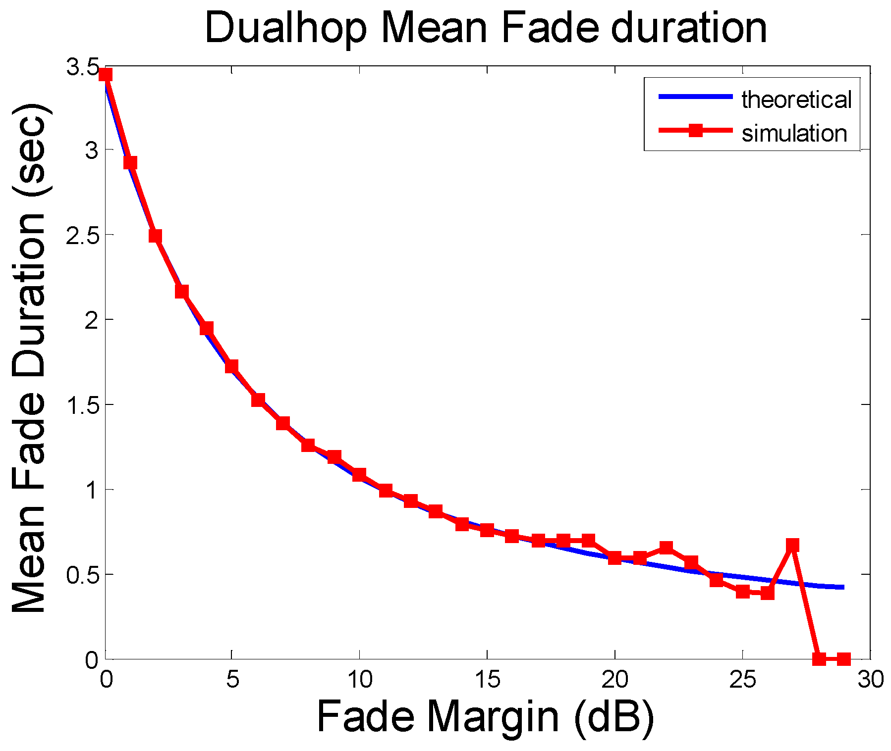
In Figure 3 we plot the theoretical alongside the simulated by use of the model outage probability for the case of the decode and forward dual-hop relay. The accuracy with which the model generates the stationary statistical characteristics of second order is remarkable. The efficiency of the model concerning the second order dynamical statistical characteristics is shown in Figure 4 where the theoretically calculated in Section 2.4 average outage duration is plotted along with the generated one for different values of fade margin. The simulated values are in a very good agreement with the theoretical ones. Slight differences are noted for high values of fade margin, which are due to the slow convergence of the simulated AOD for such high values of fade margin. Figure 4 serves also as a validation for the theoretical derivation of the AOD as in Section 2.4.

In Figure 5, in order to show the impact of the shadowing correlation coefficient we plot the theoretical AOD for three different values of the correlation coefficient. From Figure 5 we see that the impact of the shadowing correlation coefficient is very small concerning the average outage duration.

3.2. Cellular Network

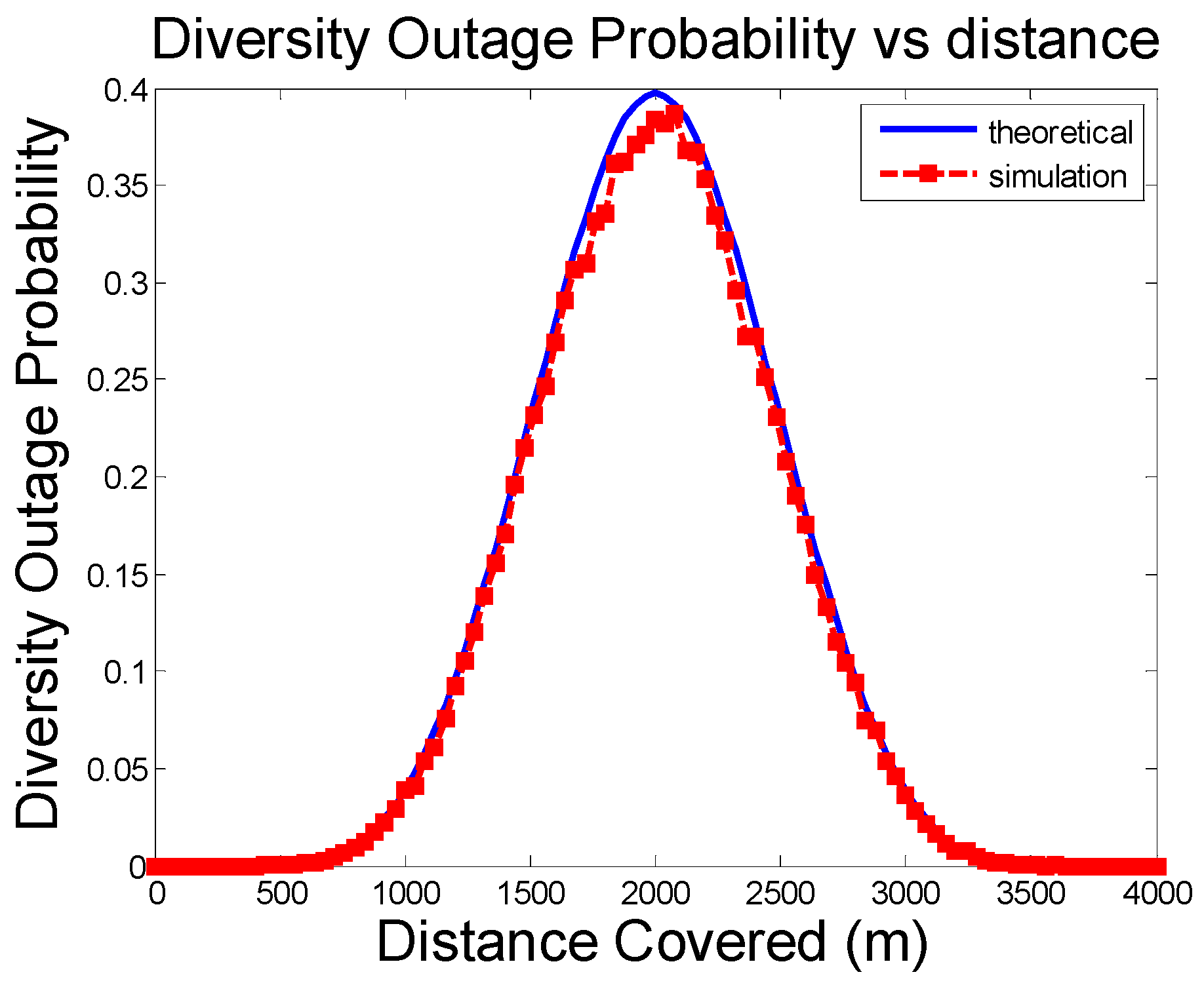
The second numerical application of the model refers to an outdoor cellular network in an urban environment. The scenario consists of a mobile station MS moving along the trajectory from point A to point B passing through the mid-point of two base stations BS1 and BS2. The distance between the base stations is 4 km. The base stations are supposed to transmit with the same characteristics. The propagation loss model used for the subsequent variation of the received power is COST231-HATA. The location variability has been chosen as 6 dB and the shadowing decorrelation distance 10 m. The frequency of operation considered is 3.5 GHz and the mobile is supposed to be moving with the typical speed for vehicular in urban areas of 14 m/s.

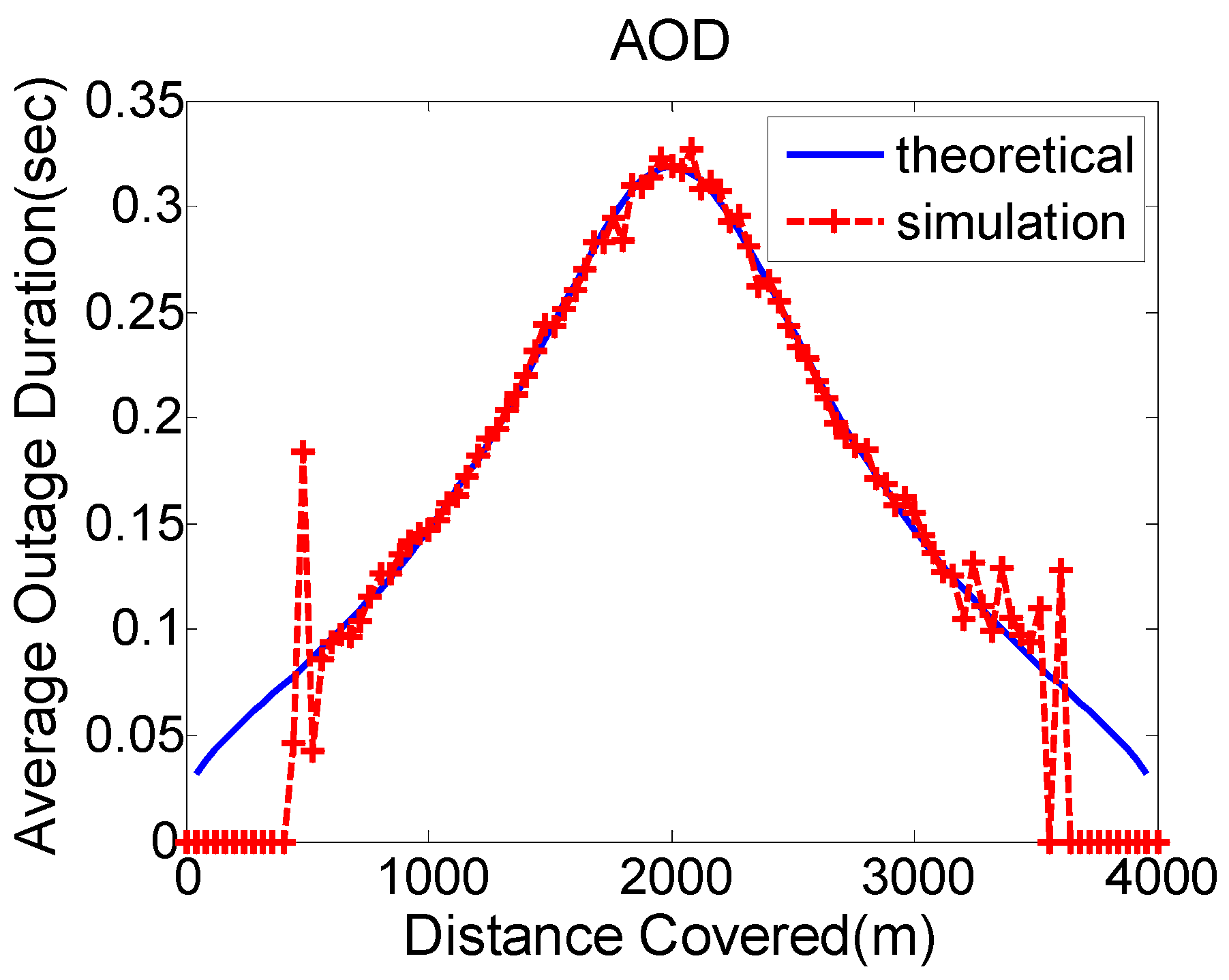
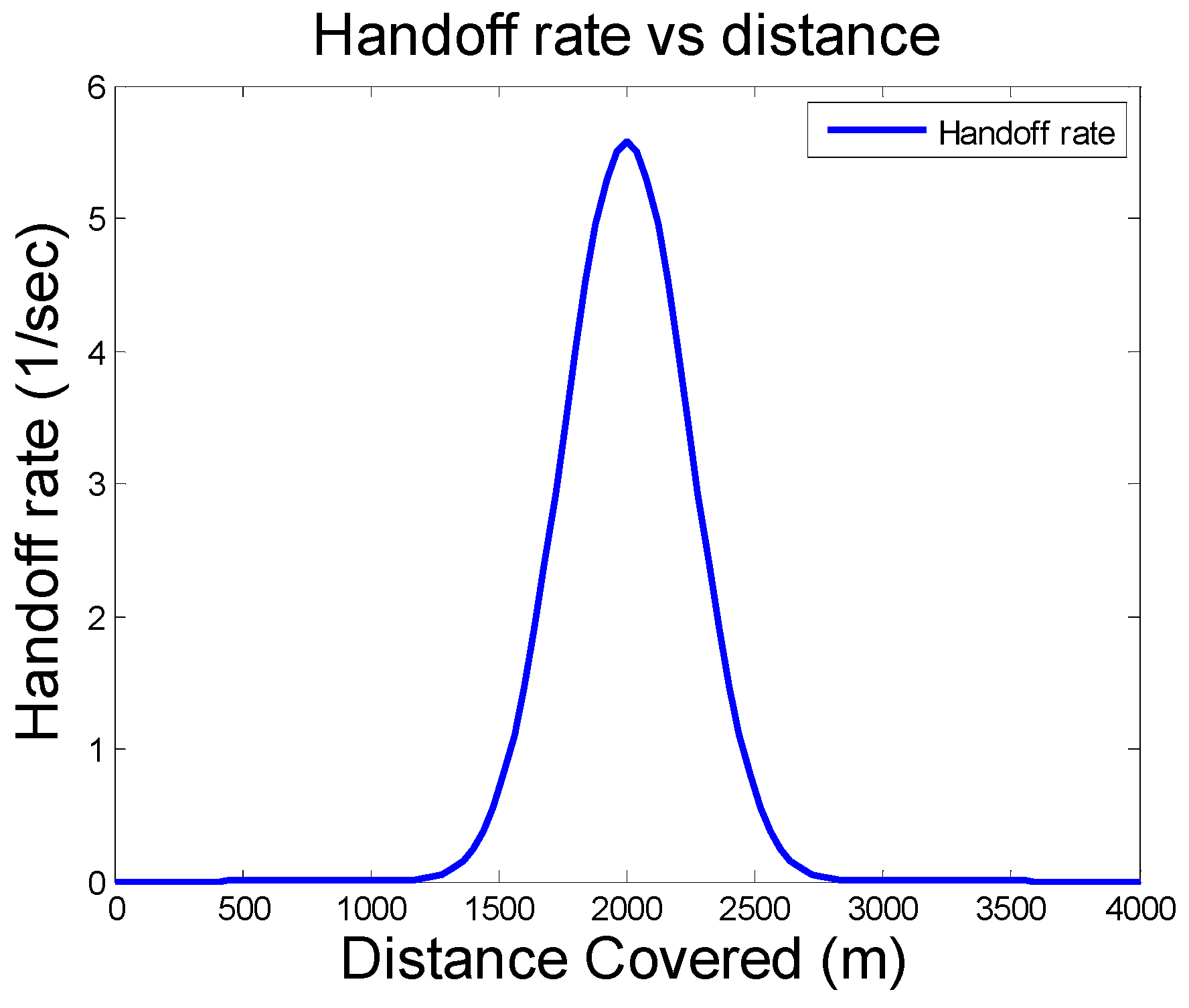
In Figure 6 we plot the theoretical and the simulated outage probability for dual diversity reception from the signals of the two base stations versus distance covered. The dynamic model generates the dual diversity outage probability with great accuracy. Maximum values are noticed as expected in the mean distance between the two base stations. In the same conclusion we arrive for the case of the AOD shown in Figure 7. Here we note again the fact that the simulated AOD does not converge for high values of fade margin near the two base stations. Finally in Figure 8 we plot the hand-off rate. This is defined as a kind of LCR when the strongest signal becomes weaker. The receiver selects in each time instant the strongest signal from the two base stations. As expected the bigger hand-off rate is noticed in the mean distance between the two base stations.

4. Conclusions

In this paper, there has been presented a novel dynamic model, able to take into account the fluctuations of shadowing in a statistical basis. The main assumption of the modeling as validated from experimental results is the joint lognormality of the related shadowing values. The new dynamic channel model framework may be used for the effective and realistic design of new wireless systems by providing simulated time series for testing, as well as in the implementation of fade mitigation techniques. The model can effectively be used in the accurate design and analysis of modern wireless systems including 5G cellular wireless systems, MIMO systems, diversity (transmit, reception, cooperative) schemes, ad-hoc networks, multi-hop wireless, collaborative cognitive radios, body area networks, and in every other aspect of wireless networking, where correlated shadowing has a major impact on system’s performance. The proposed model can also be incorporated in transitions state models LOS/NLOS (blockage or not) state transition modeled as a Markov chain. Moreover, with a view not referring to specific equipment characteristics, the numerical results have been presented in relation to the fade margin.

References

- Rappaport, T.S.; Sun, S.; Mayuz, R.; Zhao, H.; Azar, Y.; Wang, K.; Wong, G.N.; Schulz, J.K.; Samimi, M.; Gutierez, F. Millimeter wave mobile communications for 5G cellular: It will work! IEEE Access J. 2013, 1, 335–349. [Google Scholar] [CrossRef]
- Rappaport, T.S.; Gutierez, F.; Dor, B.E.; Murdokc, J.N.; Qiao, Y.; Tamir, J.I. Broadband millimeter wave propagation measurements and models using adaptive-beam antennas for outdoor urban cellular communications. IEEE Trans. Antennas Propag. 2013, 61, 1850–1859. [Google Scholar] [CrossRef]
- Ghosh, A.; Thomas, T.A.; Cudak, M.C.; Ratasuk, R.; Moorut, P.; Vook, F.W.; Rappaport, T.S.; Sun, S.; Nie, S. Millimeter wave enhanced local area systems: A high data-rate approach for future wireless networks. IEEE J. Sel. Areas Commun. 2014, 32, 1152–1163. [Google Scholar] [CrossRef]
- Thompson, J.; Ge, X.; Wu, H.C.; Irmer, R.; Jiang, H.; Fettweis, G.; Alamouti, S. 5G wireless communication systems: Prospects and challenges. Commun. Mag. 2014, 52, 62–64. [Google Scholar] [CrossRef]
- Sun, S.; Rappaport, T.S.; Shafi, M.; Tang, P.; Zhang, J.; Smith, P.J. Propagation models and performance evaluation for 5G millimeter-wave bands. IEEE Trans. Veh. Technol. 2018, 67, 8422–8439. [Google Scholar] [CrossRef]
- Iyanda Sulyman, A.; Alwarafy, A.; MacCartney, G.R.; Rappaport, T.S.; Alsanie, A. Directional radio propagation path loss models for millimeter-wave wireless networks in the 28-, 60 and 73-GHz Bands. IEEE Trans Wirel. Commun. 2016, 35, 6939–6947. [Google Scholar] [CrossRef]
- Rappaport, T.S. Wireless Communications; Prentice Hall PTR: Upper Saddle River, NJ, USA; London, UK, 2001. [Google Scholar]
- Liberti, J.C.; Rappaport, T.S. Statistics of shadowing in indoor radio channels at 900 and 1900 MHz. In Proceedings of the 1992 IEEE Military Communications Conference, MILCOM 92 Conference Record, Communications—Fusing Command, Control and Intelligence, San Diego, CA, USA, 11–14 October 1992; pp. 1066–1070. [Google Scholar]
- Szyszkowicz, S.S.; Yanikomeroglu, H.; Thompson, J.S. On the Feasibility of wireless shadowing correlation models. IEEE Trans. Veh. Technol. 2010, 59, 4222–4236. [Google Scholar] [CrossRef]
- Catrein, D.; Mathar, R. Gaussian random fields as a model for spatially correlated log-normal fading. In Proceedings of the Telecommunication Networks and Applications Conference, Adelaide, Australia, 7–10 December 2008; pp. 153–157. [Google Scholar]
- Cai, X.; Giannakis, G.B. A two-dimensional channel simulation model for shadowing processes. IEEE Trans. Veh. Technol. 2003, 52, 1558–1567. [Google Scholar]
- Fraile, R.; Monserrat, J.F.; Gozálvez, J.; Cardona, N. Mobile radio bi-dimensional large-scale fading modelling with site-to-site cross-correlation. Eur. Trans. Telecommun. 2008, 19, 101–106. [Google Scholar] [CrossRef]
- Patwari, N.; Agrawal, P. NeSh: A joint shadowing model for links in a multi-hop network. In Proceedings of the IEEE International Conference on Acoustics, Speech and Signal Processing (ICASSP), Las Vegas, NV, USA, 31 March–4 April 2008; pp. 2873–2876. [Google Scholar]
- Forkel, I.; Schinnenburg, M.; Ang, M. Generation of Two-dimensional correlated shadowing for mobile radio network simulation. In Proceedings of the 7th International Symposium on Wireless Personal Multimedia Communications (WPMC), Abano Terme, Italy, 12–15 September 2004. [Google Scholar]
- Seetharam, A.; Kurose, J.; Goeckel, D.; Bhanage, G. A Markov chain model for coarse timescale channel variation in an 802.16e wireless network. In Proceedings of the IEEE INFOCOM, Orlando, FL, USA, 25–30 March 2012; pp. 1800–1807. [Google Scholar]
- Mukherjee, S.; Avidor, D. Dynamics of path losses between a mobile terminal and multiple base stations in a cellular environment. IEEE Trans. Veh. Technol. 2001, 50, 1590–1603. [Google Scholar] [CrossRef]
- Hashemi, H. The indoor radio propagation channel. Proc. IEEE 1993, 81, 943–968. [Google Scholar] [CrossRef]
- Kashiwagi, I.; Taga, T.; Imai, T. Time-Varying path-shadowing model for indoor populated environments. IEEE Trans. Veh. Technol. 2010, 59, 16–28. [Google Scholar] [CrossRef]
- Zhang, R.; Cai, L. A Markov model for indoor ultra-wideband channel with people shadowing. Mob. Netw. Appl. 2007, 12, 438–449. [Google Scholar] [CrossRef]
- Klingenbrunn, T.; Mogensen, P. Modelling cross-correlated shadowing in network simulations. In Proceedings of the IEEE VTS 50th Vehicular Technology Conference, VTC 1999—Fall, Amsterdam, The Netherlands, 19–22 September 1999; pp. 1407–1411. [Google Scholar]
- Butterworth, K.S.; Sowerby, K.W.; Williamson, A.G. Base station placement for in-building mobile communication systems to yield high capacity and efficiency. IEEE Trans. Commun. 2000, 48, 658–669. [Google Scholar] [CrossRef]
- Jalden, N.; Zetterberg, P.; Ottersten, B.; Hong, A.; Thoma, R. Correlation Properties of large scale fading based on indoor measurements. In Proceedings of the IEEE Wireless Communications and Networking Conference (WCNC), Kowloon, China, 11–15 March 2007; pp. 1894–1899. [Google Scholar]
- Patwari, N.; Wang, Y.; O’Dea, R.J. The importance of the multipoint-to-multipoint indoor radio channel in ad hoc networks. In Proceedings of the IEEE Wireless Communications and Networking Conference (WCNC2002), Orlando, FL, USA, 17–21 March 2002; pp. 608–612. [Google Scholar]
- Agrawal, P.; Patwari, N. Correlated link shadow fading in multi-hop wireless networks. IEEE Trans. Wirel. Commun. 2009, 8, 4024–4036. [Google Scholar] [CrossRef]
- Charalambous, C.D.; Menemenlis, N. Dynamical Spatial log-normal shadowing models for mobile communications. In Proceedings of the XXVIIth Triennial General Assembly of the International Union of Radio Science (URSI), Maastricht, The Netherlands, 17–24 August 2002; pp. 1–4. [Google Scholar]
- Skraparlis, D.; Sakarellos, V.K.; Panagopoulos, A.D.; Kanellopoulos, J.D. Outage performance analysis of cooperative diversity with MRC and SC in Correlated lognormal channels. EURASIP J. Wirel. Commun. Netw. 2009, 2009, 707839. [Google Scholar] [CrossRef]
- Skraparlis, D.; Sakarellos, V.; Panagopoulos, A.D.; Kanellopoulos, J.D. Performance of N-branch receive diversity combining in correlated lognormal channels. IEEE Commun. Lett. 2009, 13, 489–491. [Google Scholar] [CrossRef]
- Skraparlis, D.; Sakarellos, V.; Sandell, M.; Panagopoulos, A.D.; Kanellopoulos, J.D. On the effect of correlation on the performance of dual diversity receivers in lognormal fading. IEEE Commun. Lett. 2010, 14, 1038–1040. [Google Scholar] [CrossRef]
- Sakarellos, V.; Skraparlis, D.; Panagopoulos, A.D.; Kanellopoulos, J.D. Cooperative Diversity Performance of Selection Relaying over Correlated Shadowing; Elsevier Physical Communication: Amsterdam, The Netherlands, 2011; pp. 182–189. [Google Scholar]
- Skraparlis, D.; Sakarellos, V.K.; Panagopoulos, A.D.; Kanellopoulos, J.D. New results on the statistics and the capacity of dual-branch MRC and EGC Diversity in correlated lognormal channels. IEEE Commun. Lett. 2011, 15, 617–619. [Google Scholar] [CrossRef]
- Sakarellos, V.K.; Skraparlis, D.; Panagopoulos, A.D.; Kanellopoulos, J.D. Cooperative Diversity performance in millimeter wave radio systems. IEEE Trans. Commun. 2012, 60, 3641–3649. [Google Scholar] [CrossRef]
- Karagiannis, G.; Panagopoulos, A.D.; Kanellopoulos, J.D. Multi-Dimensional rain attenuation stochastic dynamic modeling: Application to earth-space diversity systems. IEEE Trans. Antennas Propag. 2012, 60, 5400–5411. [Google Scholar] [CrossRef]
- Karagiannis, G.; Panagopoulos, A.D.; Kanellopoulos, J.D. Short-term rain attenuation frequency scaling for satellite up-link power control applications. IEEE Trans. Antennas Propag. 2013, 61, 2829–2837. [Google Scholar] [CrossRef]
- Gudmundson, M. Correlation model for shadow fading in mobile radio systems. Electron. Lett. 1991, 27, 2145–2146. [Google Scholar] [CrossRef]
- Graziosi, F.; Santucci, F. A general correlation model for shadow fading in mobile radio systems. IEEE Commun. Lett. 2002, 6, 102–104. [Google Scholar] [CrossRef]
- Avidor, D.; Mukherjee, S. Hidden issues in the simulation of fixed wireless systems. Wirel. Netw. 2001, 7, 187–200. [Google Scholar] [CrossRef]
- Karatzas, I.; Shreve, S.E. Brownian Motion and Stochastic Calculus; Springer: New York, NY, USA, 1991; Volume 113, p. 470. [Google Scholar]
- Graziosi, F.; Santucci, F. Distribution of outage intervals in macrodiversity cellular systems. IEEE J. Sel. Areas Commun. 1999, 17, 2011–2021. [Google Scholar] [CrossRef]
- Rice, S.O. Distribution of the duration of fades in radio transmission: Gaussian noise model. Bell Syst. Tech. J. 1958, 37, 581–635. [Google Scholar] [CrossRef]
- Stratonovich, R.L.; Silverman, R.A. Topics in the Theory of Random Noise; Revis Engl; Gordon and Breach: New York, NY, USA, 1967. [Google Scholar]
- Giancristofaro, D. Correlation model for shadow fading in mobile radio channels. Electron. Lett. 1996, 32, 958–959. [Google Scholar] [CrossRef]
- Stüber, G.L. Principles of Mobile Communication; Kluwer Academic: Boston, MA, USA, 2001; Volume 2, p. 752. [Google Scholar]
- Jeon, N.-R.; Kim, K.-H.; Choi, J.-H.; Kim, S. A Spatial correlation model for shadow fading in indoor multipath propagation. In Proceedings of the Vehicular Technology Conference Fall (VTC 2010-Fall), Ottawa, ON, Canada, 6–9 September 2010; pp. 1–6. [Google Scholar]
- Belyaev, Y. On the number of exits across the boundary of a region by a vector stochastic process. Theory Probab. Appl. 1968, 13, 320–324. [Google Scholar] [CrossRef]
- Lindgren, G. Stationary stochastic processes. In Theory and Applications; Texts in Statistical Science Series; CRC Press: Boca Raton, FL, USA, 2013; p. 347. [Google Scholar]
- Adler, R.J.; Taylor, J. Random Fields and Geometry; Springer: Dordrecht, The Netherlands, 2007. [Google Scholar]
Figure 1.
Shaded area of outage for a dual-diversity scheme for selection combining (SC) method.
Figure 2.
Shaded area of outage for a regenerative dual-hop link.
Figure 3.
Theoretical and simulated outage duration for a dual-hop link vs. fade margin.
Figure 4.
Theoretical and simulated average outage duration for a regenerative dual-hop link vs. fade margin.
Figure 5.
Average outage duration for a regenerative dual-hop link vs. fade margin for three different values of shadowing correlation coefficient.
Figure 6.
Theoretical and simulated outage duration for a dual diversity scheme vs. distance covered.
Figure 7.
Theoretical and simulated average outage duration for a dual diversity scheme vs. distance covered.
Figure 8.
Average hand-off rate for a mobile receiver moving between two base stations.
© 2019 by the authors. Licensee MDPI, Basel, Switzerland. This article is an open access article distributed under the terms and conditions of the Creative Commons Attribution (CC BY) license (http://creativecommons.org/licenses/by/4.0/).
Share and Cite
MDPI and ACS Style
Karagiannis, G.A.; Panagopoulos, A.D. Dynamic Lognormal Shadowing Framework for the Performance Evaluation of Next Generation Cellular Systems. Future Internet 2019, 11, 106. https://doi.org/10.3390/fi11050106
AMA Style
Karagiannis GA, Panagopoulos AD. Dynamic Lognormal Shadowing Framework for the Performance Evaluation of Next Generation Cellular Systems. Future Internet. 2019; 11(5):106. https://doi.org/10.3390/fi11050106
Chicago/Turabian StyleKaragiannis, Georgios A., and Athanasios D. Panagopoulos. 2019. "Dynamic Lognormal Shadowing Framework for the Performance Evaluation of Next Generation Cellular Systems" Future Internet 11, no. 5: 106. https://doi.org/10.3390/fi11050106
Note that from the first issue of 2016, this journal uses article numbers instead of page numbers. See further details here.