Smart System for Prediction of Accurate Surface Electromyography Signals Using an Artificial Neural Network

Abstract

Bioelectric signals are used to measure electrical potential, but there are different types of signals. The electromyography (EMG) is a type of bioelectric signal used to monitor and recode the electrical activity of the muscles. The current work aims to model and reproduce surface EMG (SEMG) signals using an artificial neural network. Such research can aid studies into life enhancement for those suffering from damage or disease affecting their nervous system. The SEMG signal is collected from the surface above the bicep muscle through dynamic (concentric and eccentric) contraction with various loads. In this paper, we use time domain features to analyze the relationship between the amplitude of SEMG signals and the load. We extract some features (e.g., mean absolute value, root mean square, variance and standard deviation) from the collected SEMG signals to estimate the bicep’ muscle force for the various loads. Further, we use the R-squared value to depict the correlation between the SEMG amplitude and the muscle loads by linear fitting. The best performance the ANN model with 60 hidden neurons for three loads used (3 kg, 5 kg and 7 kg) has given a mean square error of 1.145, 1.3659 and 1.4238, respectively. The R-squared observed are 0.9993, 0.99999 and 0.99999 for predicting (reproduction step) of smooth SEMG signals.

1. Introduction

Humans rely on a healthy nervous system to control their movements. When their muscles react to nerve impulses (electrical signals) sent by the brain in cases of injury and nerve diseases, this important link can be broken. Understanding the signals between the muscles and the brain could have a significant impact on improving the lives of those suffering from nerve diseases or nerve damage. In this paper, we start by measuring the bioelectrical signals at the bicep and then develop a model using an artificial neural network (ANN).

Several techniques are used to observe bioelectrical signals and electrical activity of the human body; some examples are the electrocardiogram (ECG), electroencephalogram (EEG) and electromyography (EMG). The peak amplitude of electromyography (EMG) signals is very low (a few microvolts), thus, such signals need to be amplified to sense it and it also needs to be converted from the analog (continuous) form to a digital (discrete) form to record it in a computer for further processing. This research will measure the muscle electrical activity using Surface Electromyography (SEMG), which involves placing electrodes on the skin to capture the electrical activity of the muscle and record it in a computer after amplifying and converting it to a digital signal [1].

The current research will focus on measuring electrical activity of the bicep muscle during dynamic contraction (concentric and eccentric contraction). Such bicep activity is important in a variety of tasks involving rotation of the forearm around the elbow joint. The recorded weak electrical signals naturally contain unwanted information (that is noise) from wide spectrum of sources such as electronic equipment and physiological factors. This research will further process the SEMG signals to extract smooth signals by applying a low pass filter after determining the cutoff frequency utilizing the fast Fourier transform (FFT).

The main objective of this research is to model nerve signals for the human bicep muscle for future smart systems. Since SEMG is nonlinear in nature, this research will use an artificial neural network (ANN) to predict it.

Related Work

In the last few years, several works involving modelling the EMG signal have been investigated in areas such as motion recognition and force estimation.

Jali et al. [2] has introduced a model that illustrates the correlation between muscle EMG signal and torque using ANN techniques. For that, EMG signals from biceps muscles are collected and later used to estimate the elbow joint torque temporal values. As a preprocessing step, the authors used a low-pass filter with a cutoff frequency of 10 Hz. Further, a DC offset is subtracted from the collected signals before they are rectified to obtain its absolute value. The transformed signals are then smoothed and normalized through having them pass through a fifth-order Butterworth-type low-pass filter. Smoothed signals are then modeled using a two-layer feed-forward neural network. In this regard, the ANN is trained using a back propagation neural network (BPNN). The performance of the introduced procedure is determined through calculating the mean square error (MSE) and regression ($R^2$). The proposed model demonstrated an MSE of $1.7638e^{-11}$ at epoch 1000 and average regression of 1.000 [2].

Ullah et al. [3] presented a new mathematical equation to model the elbow joint torque from the electromyography (EMG) signal. Again, preprocessing is done to (i) remove the DC offset, (ii) remove 60 Hz of noise and (iii) estimate the smoothed EMG signal amplitude. The detected amplitude is later mapped to joint-torque using a novel nonlinear interpolation equation. An experimental set of 10 subjects was used during experiments, each of which has performed variable force maximal voluntary contractions (MVC) and submaximal voluntary contractions (SMVC). The experimental results obtained from this study are observed to be correlated to the true values of the torque with the average correlation and MSE for different experiments are 0.9997 and 0.047 Newton meter (Nm); respectively.

In Wang et al. [4], the authors introduced a procedure model muscle activation from EMG signals, again using neural network techniques. The authors predict muscle activations from temporal EMG signals without constructing complex mathematical models to model muscle activation dynamics. The NN model of muscle activation applied in this work is of four layers and utilizes an improved back-propagation for the training step. Joint torque was calculated from EMG signals collected from ten flexor and extensor muscles. A musculoskeletal geometry model is built to obtain moment arms, from which joint moments were estimated comparatively evaluated against measured values. Study results successfully represent the relationship between EMG signals and joint moments.

In Yahya et al. [5], the authors have extracted several features of temporal EMG signals during hand-lifting of several loads. The authors suggested that interpreting EMG signals in time domain through feature extraction is better than studying those signals in frequency domain. In that regard, a set of four different features have been extracted. Those are: IEMG, MAV, VAR and RMS. The average muscle force condition is calculated based on the EMG signal peak amplitude and the full-wave rectification method. The R² value is used to depict the correlation between the EMG signal amplitude with the muscle load. The extracted IEMG feature is chosen as a reference feature for estimating of muscle force with R-squared value of 0.997.

In Darmakusuma et al. [6], the authors utilized the MAV method to estimate bicep force based on a collected set of surface electromyography (SEMG) signals. For that, different loads have been applied on the targeted muscle. Those are: zero, 2 kg, 3 kg, 4 kg and 5 kg. Noise in SEMG signals was reduced by having them pass through a Butterworth band-pass filter (BPF) with low and high cutoff frequencies of 10 Hz and 40 Hz, respectively. The authors used the mean absolute value (MAV) method to estimate the average muscle’s force based on the SEMG voltage amplitude. The ultimate goal was to represent three states of arm muscles; (i) arm in rest, (ii) lifted arm without load and (iii) lifted arm with load.

The authors in Manimegalai et al. [7] observed that detecting human hand gestures prove useful for classification purposes. Specific patterns are extracted from EMG signals for each human arm movement and, later, a set of features were extracted those patterns and later feed to a neural network for training and classification. Those features are: mean absolute value (MAV), root mean square (RMS), Variance (VAR), Standard deviation (STD), Mean frequency (MF), Zero crossing (ZC) and Slope signal change (SSC). The ANN, in turn, classifies signals from the gestures. The authors noticed that the efficiency of classification can be improved if more signals are feed to NN. The average for the best overall training is reported in this word was 83.5%.

The authors in Ahsan et al. [8] have also introduced a hand-gesture recognition technique based on temporal EMG signals. As in Manimegalai et al. [7], EMG pattern signatures were extracted from EMG signals, later using NN, EMG signals were classified on those extracted features. The authors have used a back-propagation (BP) NN with Levenberg-Marquardt training to detect arm gestures. The features used in this research include the features used in Manimegalai et al. [7]. In addition, the authors used added the wavelet length (WL) feature. In this work, EMG signals were classified with an average success rate of 88.4%.

Ganesh et al. [8], proposed using technique of sEMG based in independent component analysis (ICA). The technique used blind source separation (BSS) methods, assumptions used may affect the precision of the results, for example the BSS model assumes that the mixing process is linear but in real, it can be not. In [8] and Naik et al. [9], the ICA was used with many assumptions for example: the sources are independent and stationary, etc. In our current work, most of these assumptions were replaced with case facts.

In Ganesh et al. [8], the analysis was performed for only three-finger flexion action even though the results indicated have motivated our work for the existence of clear separation of patterns of sEMG. Sredhar et al. [10] proofed the association between the sEMG and force of muscle contraction is accepted. Mira et al. [11], conducted a study of the effects of a combined endurance training on fatigue kinetics during and immediately after a fatigue test. Recommending further study and methods, Robin et al. [12] studied twelve young men performing three exercises with full measurements for the voluntary concentric or eccentric contractions until a reduction in maximal voluntary isometric contraction (MVC) torque of at least 40% MVC was achieved immediately post-exercise.

In previous research [11,12,13], the specialists, physiology authors conducted an interesting studies in the effects of cycling training on neuromuscular fatigue and its peripheral, there work come up with outcomes which can be used in future extended work to clarify the neuromuscular function using enhanced neural network infrastructure which is used in this article, the input and the output of their work can be used as a training data for specific ANN training for further cases included in their work. Different applications could benefit from the results of this research by applying artificial neural network as in [14,15].

2. Model Design and Implementation

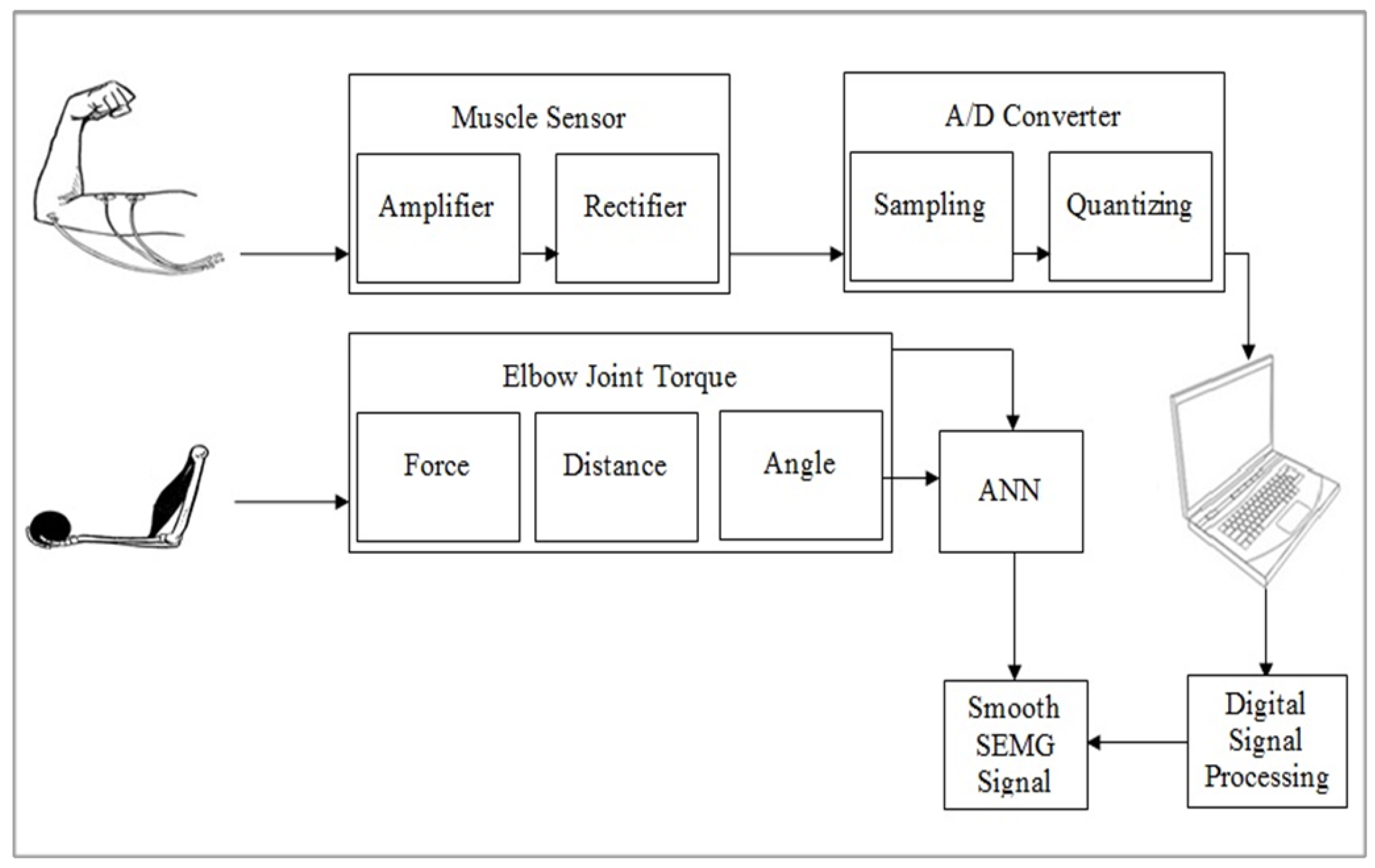
A full description for the modeling design and implementation is shown in Figure 1. The modeling design starts with collection of the SEMG signal (electrical activity) from the bicep muscle by electrodes. After converting to a digital signal, we extract a smooth signal by removing noise by converting the SEMG signal from the time domain to the frequency domain by FFT to calculate the cutoff frequency and apply a digital filter [16]. We have experimentally determined this cutoff frequency after converting the SEMG signal to the frequency domain using the Fast Fourier Transform (FFT). We set the cutoff frequency to be 10 KHz.

The smooth SEMG signal will target modeling using the ANN. The ANN will have two inputs perceptron: the first input is calculated from the torque in the third-class lever arm in the human body with load. The second input angle is calculated for every torque that causes rotation of the lower arm around the elbow joint.

2.1. Electrodes Position

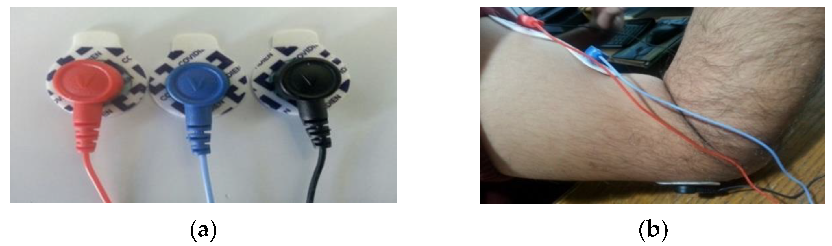
The data is collected from the bicep muscle in the right arm via three electrodes applied to human skin. They are used to capture the electrical activity during the dynamic contraction of the bicep muscle, which is the SEMG voltage signal as shown in Figure 2a. Two electrodes are effectively used to collect SEMG signal. The third electrode served as a reference (sometimes called ground electrode) [17]. Collecting high quality SEMG signals depend on (i) proper skin preparation and (ii) the position of the electrodes. Proper skin preparation is vitally important to collect high quality SEMG signals with minimal noise. The first stage involves removing the hair from the skin where the electrode will be placed. To ensure a good contact with the skin with low impedance the second stage involves cleaning the skin with alcohol. Surface electrodes are attached to the bicep muscle as shown in Figure 2b.

2.2. Materials and Set Up

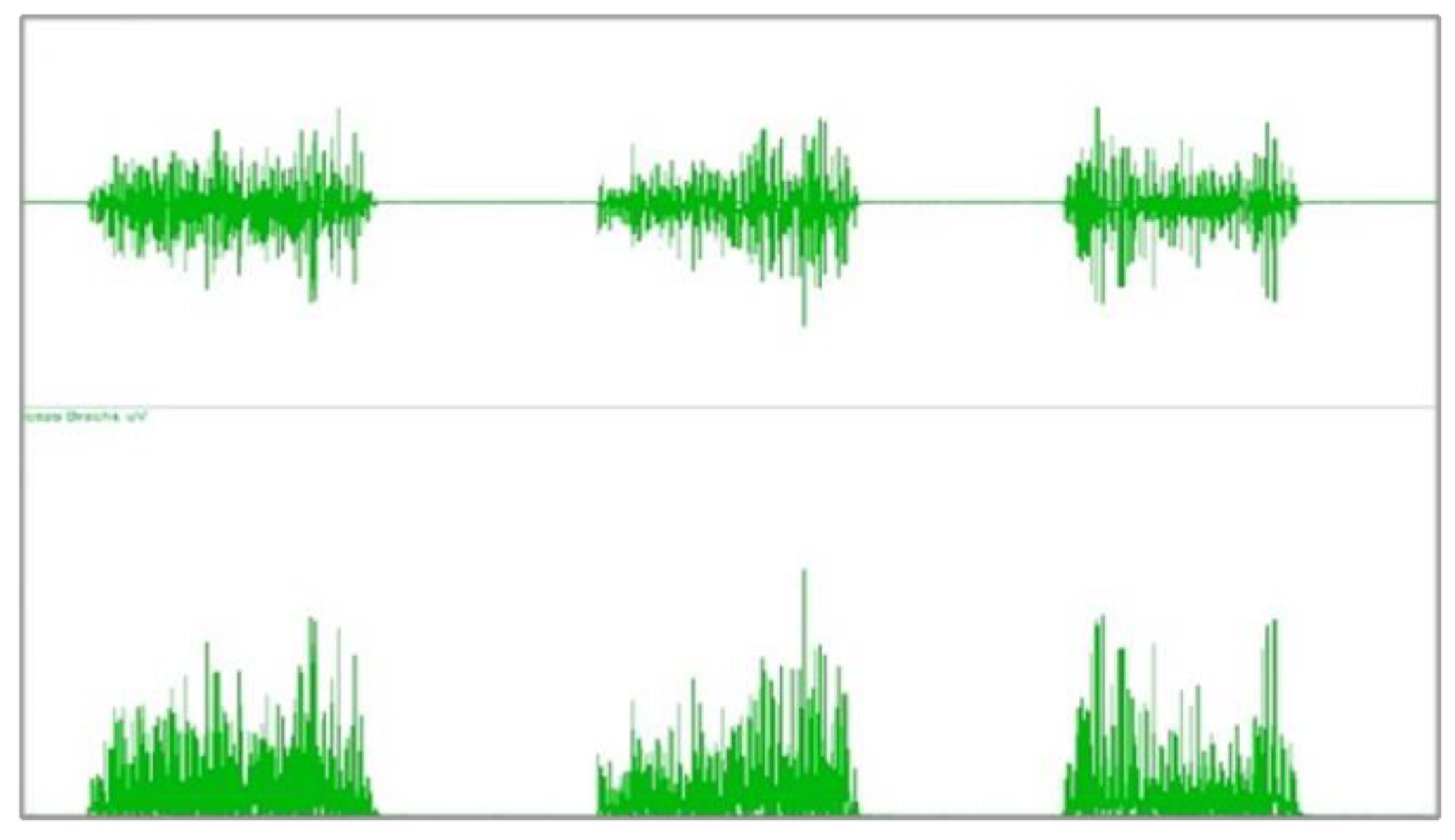
In our experiments, we use muscle sensors to rectify the SEMG signal by full wave rectification resulting in the SEMG signal as shown in Figure 3.

The output of the muscle sensor is feed to the microcontroller (ARDUINO DUE) (Figure 4) to convert the signal from analog form to digital using the controller’s A/D. Signals are sampled at a sampling rate of 1000 Hz.

2.3. The SEMG Signal Collection

The SEMG signal is recorded during the flexion and extension of the elbow joint whilst the right hand is holding a 3 kg, 5 kg and 7 kg load. These loads have been chosen because all loads that are less than 3 kg create a zero-crossing problem and all loads greater than 7 kg cannot be easily carried by the subject.

The experiment is conducted on healthy subjects who can lift the different loads. The experiment is applied on three men with different ages, weights and heights as shown in

Table 1. Three subjects with different ages, weights and heights.

Subject	Age	Weight (kg)	Height (cm)
A	36	66	168
B	31	86	182
C	25	67	166

, to find the relationship between the SEMG amplitude and the different loads with different subjects.

The subject sat on the chair while his hand was on the table. A T-square ruler was fitted on the table to get the angle ${\theta }_{\mathrm{ej}}=90°$ when the hand touches the T-square. The subject starts lifting the right hand from ${\theta }_{\mathrm{ej}}=0°$ to ${\theta }_{\mathrm{ej}}=90°$ which refers to the elbow joint without movement of the shoulder joint. The subject lifted his hand to the maximum flexion which is $90°$ and then down to the minimum extension of 0° and was holding a range of weights from 3 kg to 7 kg. There is a correlation between the angle and the time consumed in the movement. The flexion and extension of the elbow joint took 7 s divided into two stages. First stage (flexion stage) lifting the hand at ${\theta }_{\mathrm{ej}}=0°$ to ${\theta }_{\mathrm{ej}}=90°$ took 3 s. Second stage (extension stage) extension of the elbow joint back to the start point ${\theta }_{\mathrm{ej}}=0°$ took 4 s. The time used in all stages to get the high accuracy of speed with flexion and extension of the elbow joint with various loads and various subjects. The subject tried every load approximately 15 times to get the normal result, the total trial time for three loads was approximately 45 times.

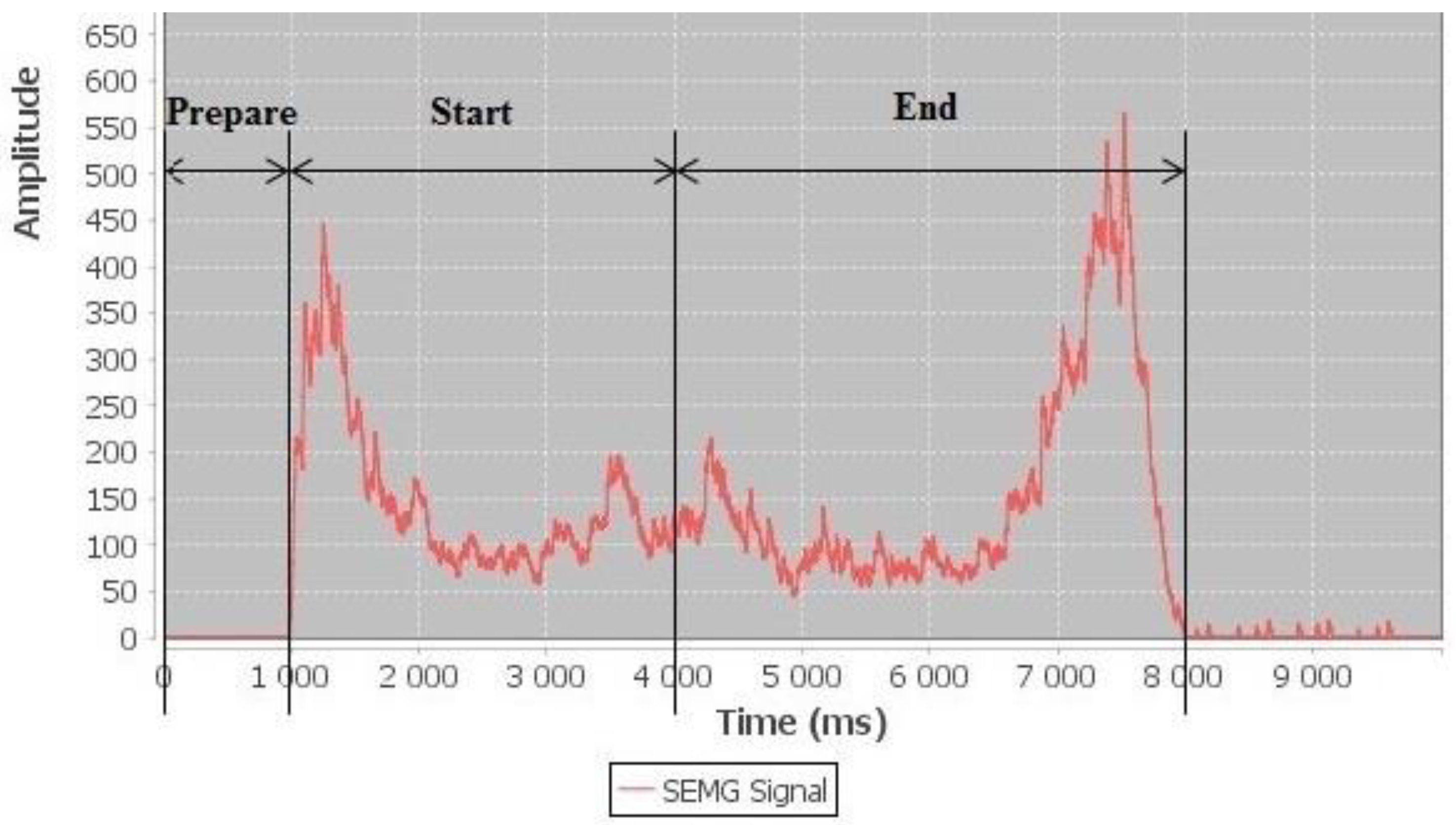
The monitoring signal is very important stage to collect the SEMG from the ARDUINO board. This stage depends on the focus subject and the muscle being relaxed. The monitoring signal captures the movement of the lower arm of the subject. The first stage is the stand by stage from interval 0 to 1 where subject stays with an angle ${\theta }_{\mathrm{ej}}=0°$ for one second. The second stage is the start stage from interval 1 to 4 s where the subject starts lifting his forearm to touch the T-square; this means the hand is starting to lifting at ${\theta }_{\mathrm{ej}}=0°$ to ${\theta }_{\mathrm{ej}}=90°$. The third stage is the end stage from interval 4 to 8 s, when the subject touches the T-square he will start lowering down his forearm to arrive to table. This means the hand is has angles between $90°$ and $0°$. When the subject arrives to the end stage the monitoring stops and the SEMG signal is recorded in the file, this is done by recoding the signal in an excel file.

2.4. Processing the SEMG Signal

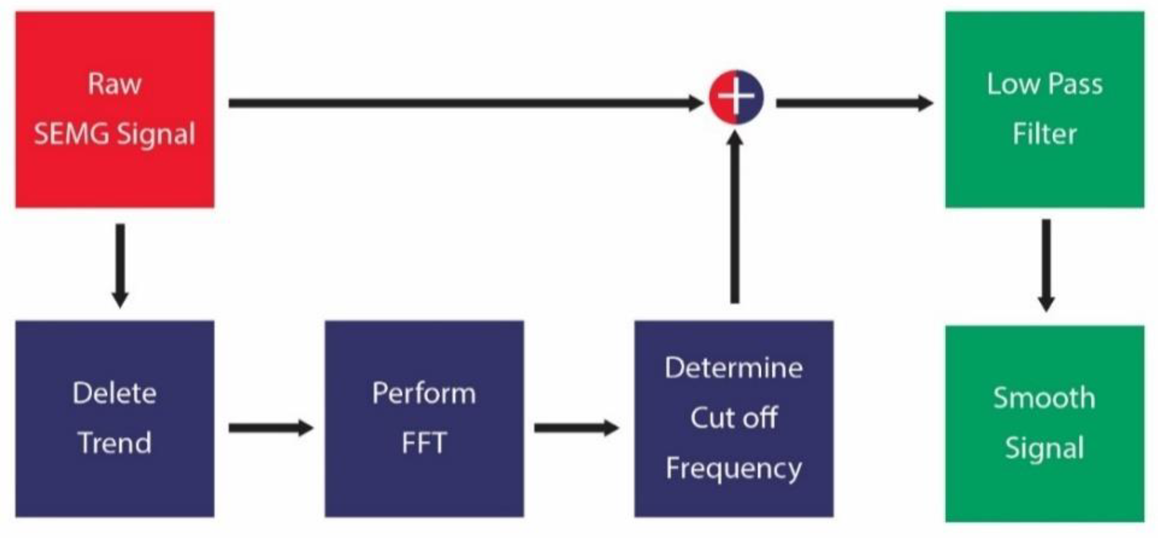
This is an important stage after the base stage of data collection because this stage plays an important role in the accuracy of the model. The SEMG contains some noise that must be removed. So, the signal was processed by removing this noise from the SEMG signal, Figure 5 shows the SEMG signal processing schematic diagram. The fast Fourier transform (FFT) is used to convert the signal from the time domain into the frequency domain, to analyses the frequency content of the signal. The signal is passed through the Butterworth filter, which is a type of low pass filter that cuts off frequencies determined to travel from the FFT to get the smooth SEMG signal.

2.5. Modeling the Nerve Signal for the Biceps Muscle

After performing the previous procedures to obtain the smoothed SEMG signal this research will build the model based on three procedures. The first procedure is extracted from the relationship between the load that is held in the hand and the bicep force. The second procedure calculates the amount of bicep force that causes rotation of the lower arm around the elbow joint at every angle of flexion. The third procedure is a predictive model to find the relationship between the target dependent variables and the independent variables. This research performs the first procedure using SEMG feature extraction to find the relationship, and the second procedure by calculation of the torque, whilst the third procedure uses the ANN.

2.5.1. SEMG Feature Extraction

In this research, five features are used to assess the relationship between the amplitude of the SEMG signal and the load of time domain features. Linear regression is used for this assessment, and then this research will decide which one of the five features has an R-squared value close to 1.00. Five features were chosen as time domain features in the assessment, as follows:

$$\mathrm{Integrated}\mathrm{EMG}(\mathrm{IEMG}):\mathrm{IEMG}={\sum }_{i=1}^N{X}_i$$

(1)

$$\mathrm{Mean}\mathrm{absolute}\mathrm{value}(\mathrm{MAV}):\mathrm{MAV}=\frac{1}{N}{\sum }_{i=1}^N{X}_i$$

(2)

$$\mathrm{Variance}(\mathrm{VAR}):\mathrm{VAR}=\frac{1}{N-1}{\sum }_i^N{X}_i^2$$

(3)

$$\mathrm{Root}\mathrm{mean}\mathrm{square}(\mathrm{RMS}):\mathrm{RMS}=\sqrt{{\sum }_i^N{X}_i^2}$$

(4)

$$\mathrm{Standard}\mathrm{deviation}(\mathrm{STD}):\mathrm{STD}=\sqrt{\frac{{\left(X-\overline{X}\right)}^2}{N-1}}$$

(5)

These features were chosen from eleven features, because MAV1, MAV2 and ZC features used as threshold. The WL feature is used to calculate the wave length but the SEMG signal is the same for three loads, and the ACC feature is the average WL. The SSI feature is the summation power of the SEMG signal and IEMG is summation SEMG so the values R-square will be the same.

2.5.2. Elbow Joint Torque

The elbow joint torque is the bicep force that causes rotation of the lower arm around the elbow joint. This research will calculate the elbow joint torque by using the stander equation as shown in Equation (6).

$$\tau =\left(r_{load}{F}_{load}\right)+\left(r_{arm}{F}_{arm}\right)\cos \theta$$

(6)

Procedures are required to analyze and find the value for all variables in the elbow joint torque. This research uses the time domain feature to find the value for force of the load ($F_{load}$) and find the mass forearm with hand ($F_{arm}$) by using the table normalized Mass and Length of body segments (standard human). The distance from load to elbow joint (${\mathrm{r}}_{\mathrm{arm}}$) means approximately the forearm length with hand.

2.5.3. Artificial Neural Network

This research used the FFNN with three layers: Input layer, Hidden layer, and Output layer. The input will have two inputs (i.e., elbow joint torque and angle flexion of the elbow joint). A single hidden layer will be used. The activation function in this ANN will be a tan sigmoid transfer function. This function will give the result between −1 and 1. The training algorithm for the FFNN will use a back-propagation algorithm to adjacent weight. To avoid an over-fitting problem the train method of MATLAB R2015a stops training when the error for the validation set starts to increase, and this research has chosen and saved the good design network, which performed best on the validation data for each load.

3. Results

The SEMG signal in this research is collected in three stages when lifting the right hand involving rotation of the elbow joint starting with flexion from ${\theta }_{\mathrm{ej}}=0°$ to ${\theta }_{\mathrm{ej}}=90°$ and then extension from ${\theta }_{\mathrm{ej}}=90°$ to ${\theta }_{\mathrm{ej}}=0°$. The first stage is the preparation stage from interval 0 to 1000 milliseconds (ms) without any movement only the subject prepares to next stage. In this stage, the angle stays ${\theta }_{\mathrm{ej}}=0°$ for one 1000 milliseconds. The second stage is the start stage from interval 1000 to 4000 MS, the subject starts lifting his forearm to reach the angle θ_ej = 90° which means his hand touches T-square; and that the forearm started lifting at ${\theta }_{\mathrm{ej}}=0°$ to ${\theta }_{\mathrm{ej}}=90°$. The third stage is the end stage from interval 4000 to 8000 MS, when the subject touches the T-square he will start lowering down his forearm to reach the table or to angle ${\theta }_{\mathrm{ej}}=0°$; this means the forearm is down at ${\theta }_{\mathrm{ej}}=90°$ to ${\theta }_{\mathrm{ej}}=0°$.

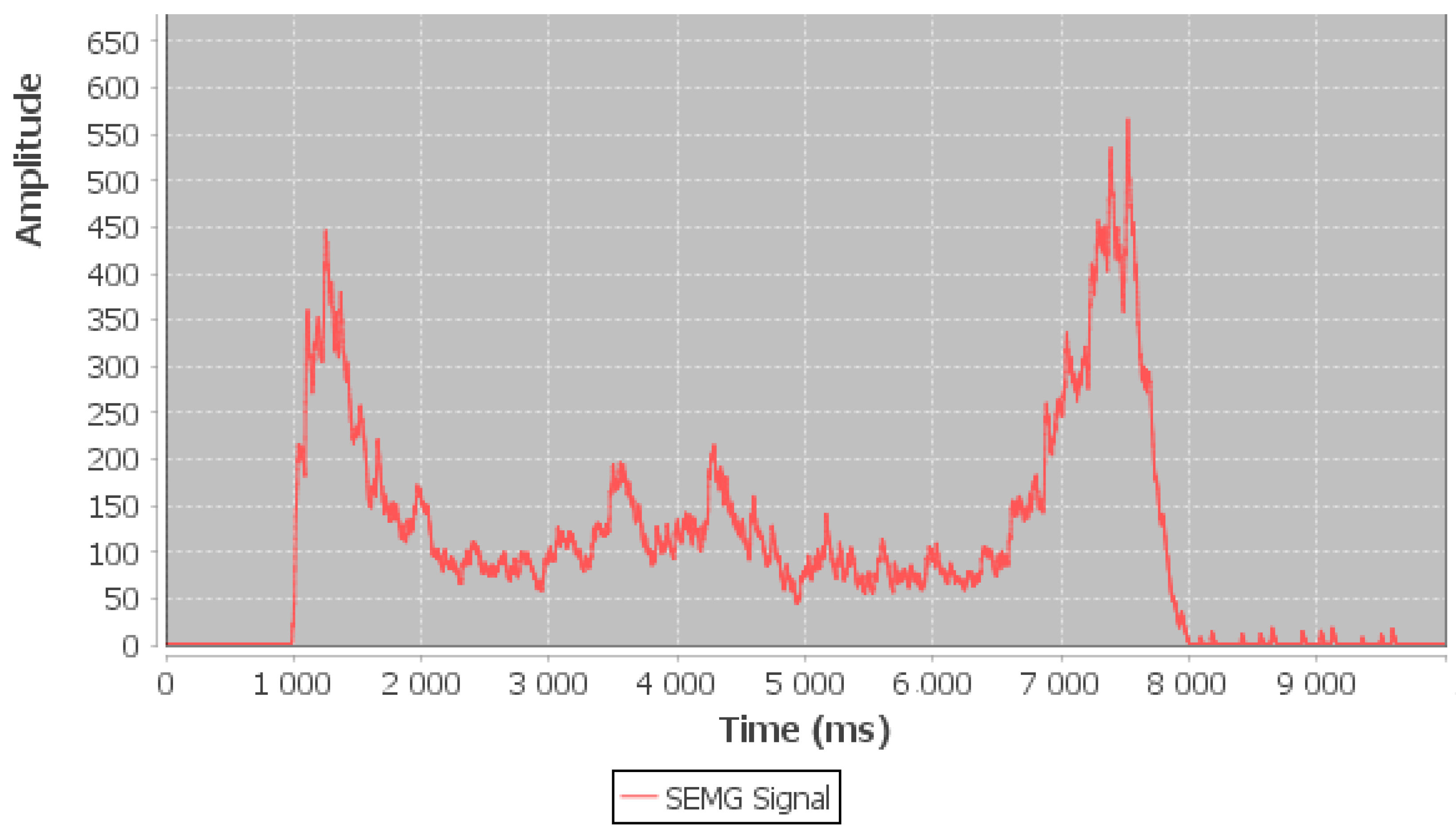
The experiment was run for three subjects with three loads: 3 kg, 5 kg and 7 kg. Figure 6 shows the raw SEMG signal for 3 kg during bicep dynamic contraction, as can be observed by the raw SEMG signal for 3 kg, when the bicep muscle starts concentric contraction and the SEMG amplitude starts increasing. Before the bicep muscle reaches the end eccentric contraction the SEMG amplitude starts increasing, in other words, the amplitude of the SEMG signal will be the maximum when the subject starts lifting their forearm and before lowering down their forearm (start and end the dynamic contraction).

The amplitude of the SEMG signal between the start and end stage of the dynamic contraction will record the minimum amplitude. This confirms the bicep muscle is being relaxed (not fatigued). Otherwise, there is a relationship between amplitude SEMG signal and load, the amplitude increases during muscle contraction when the load is increased. The amplitude of the SEMG signal for the 3 kg load is shown in Figure 7 and is the smallest one with maximum amplitude for the two types of contraction; concentric contraction with maximum amplitude 446 and eccentric contraction with maximum amplitude 566.

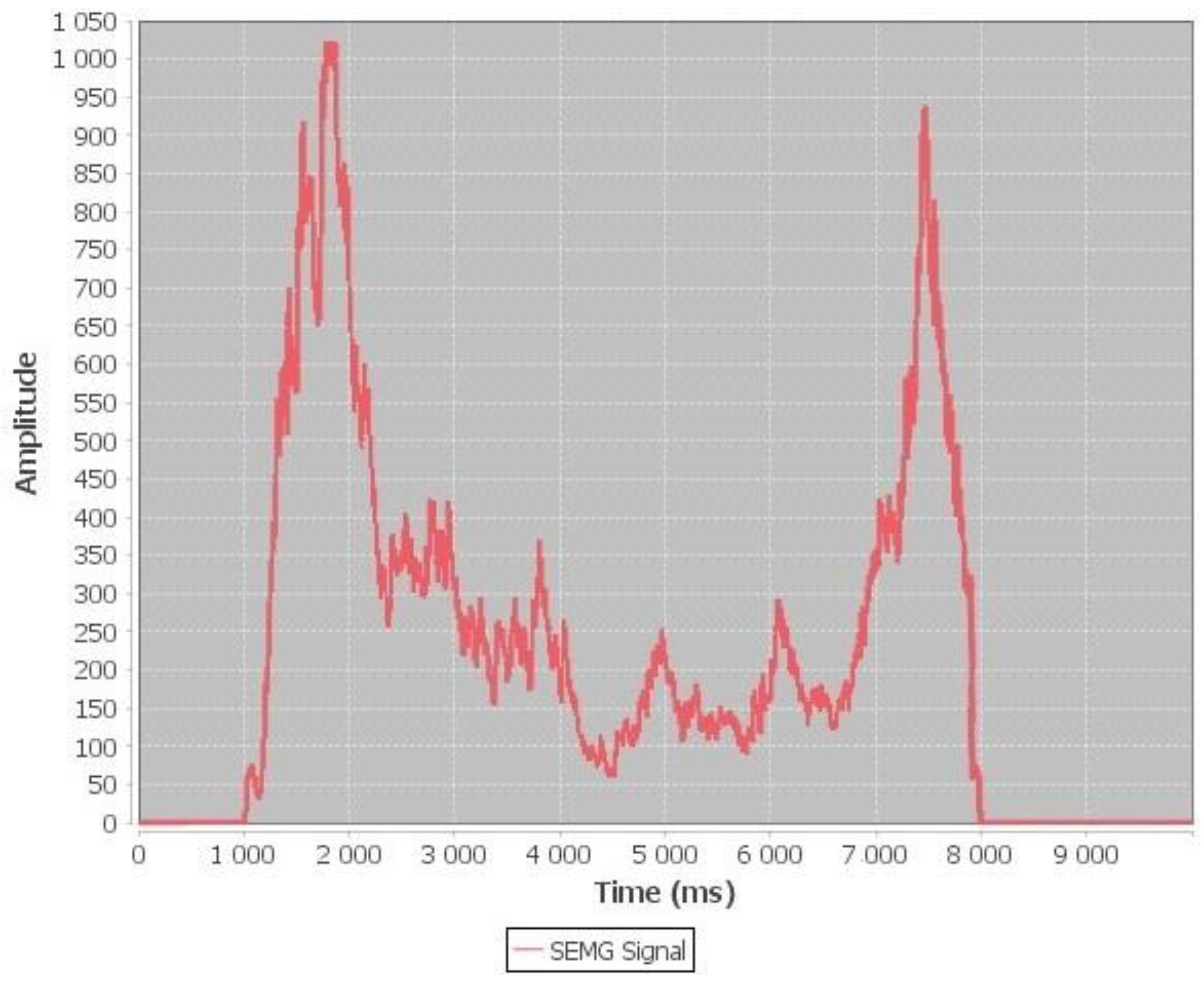
While the amplitude for the 5 kg load is higher than the 3 kg load with the maximum amplitude into two types of contraction as shown in Figure 8; concentric contraction with maximum amplitude 1023 and eccentric contraction with maximum amplitude 940. The range of amplitude for the SEMG signals is from 0–1023. The subject recoded the maximum amplitude in concentric contraction with 5 kg; this means the bicep muscle has consumed maximum effort in concentric contraction.

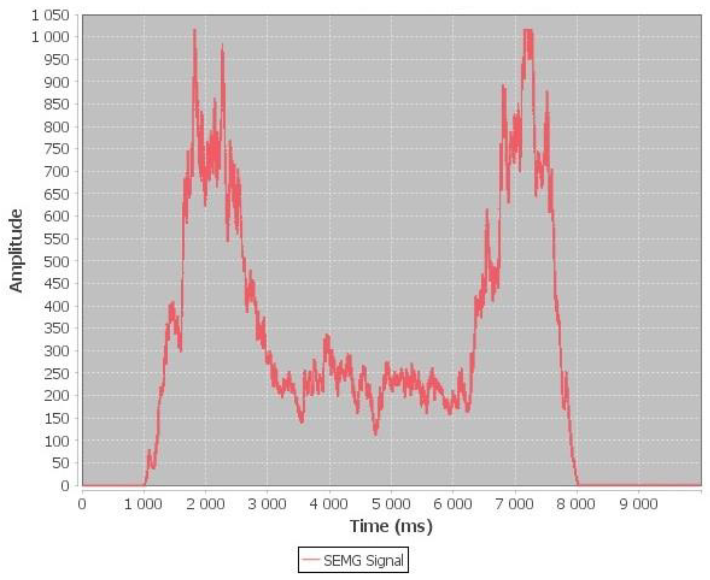
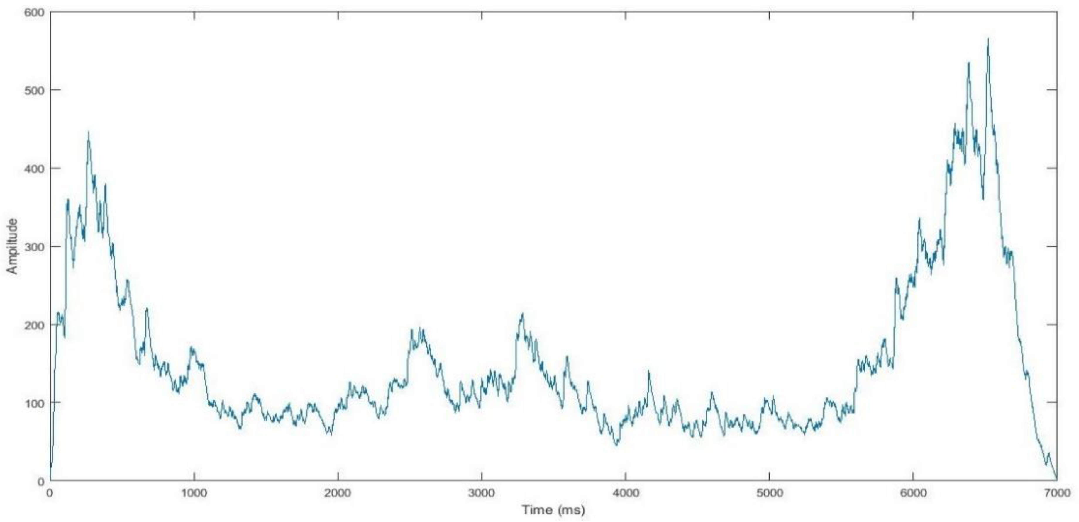
Finally, the amplitude for the 7 kg load is the highest with maximum amplitude for two types of contraction as shown in Figure 9; concentric contraction with maximum amplitude 1023 and eccentric contraction with maximum amplitude 1023. The subject recorded the maximum amplitude in concentric contraction and eccentric contraction with 7 kg; this means the bicep muscle has consumed maximum effort in concentric contraction and eccentric contraction.

3.1. Processing the SEMG Signal

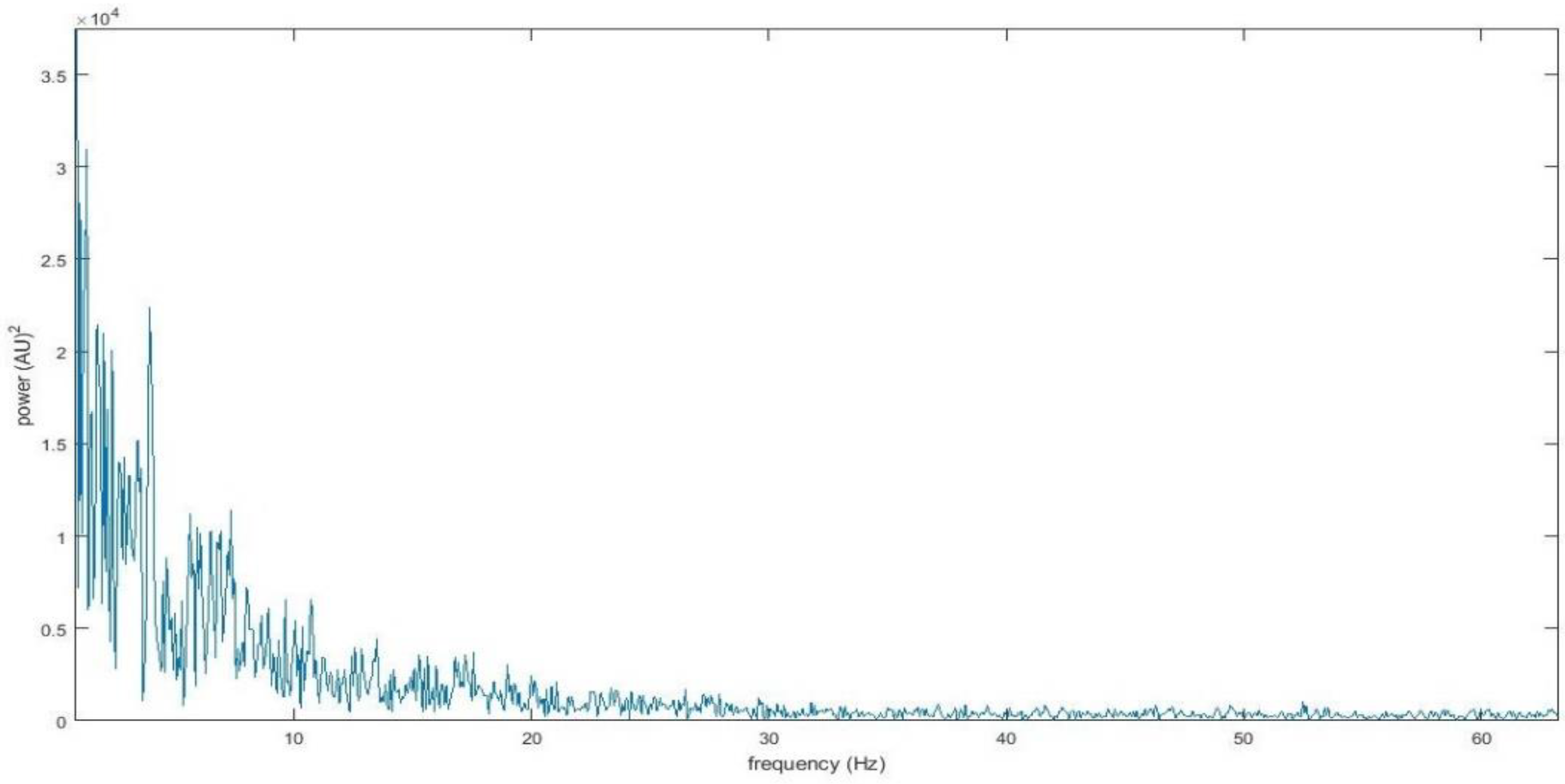
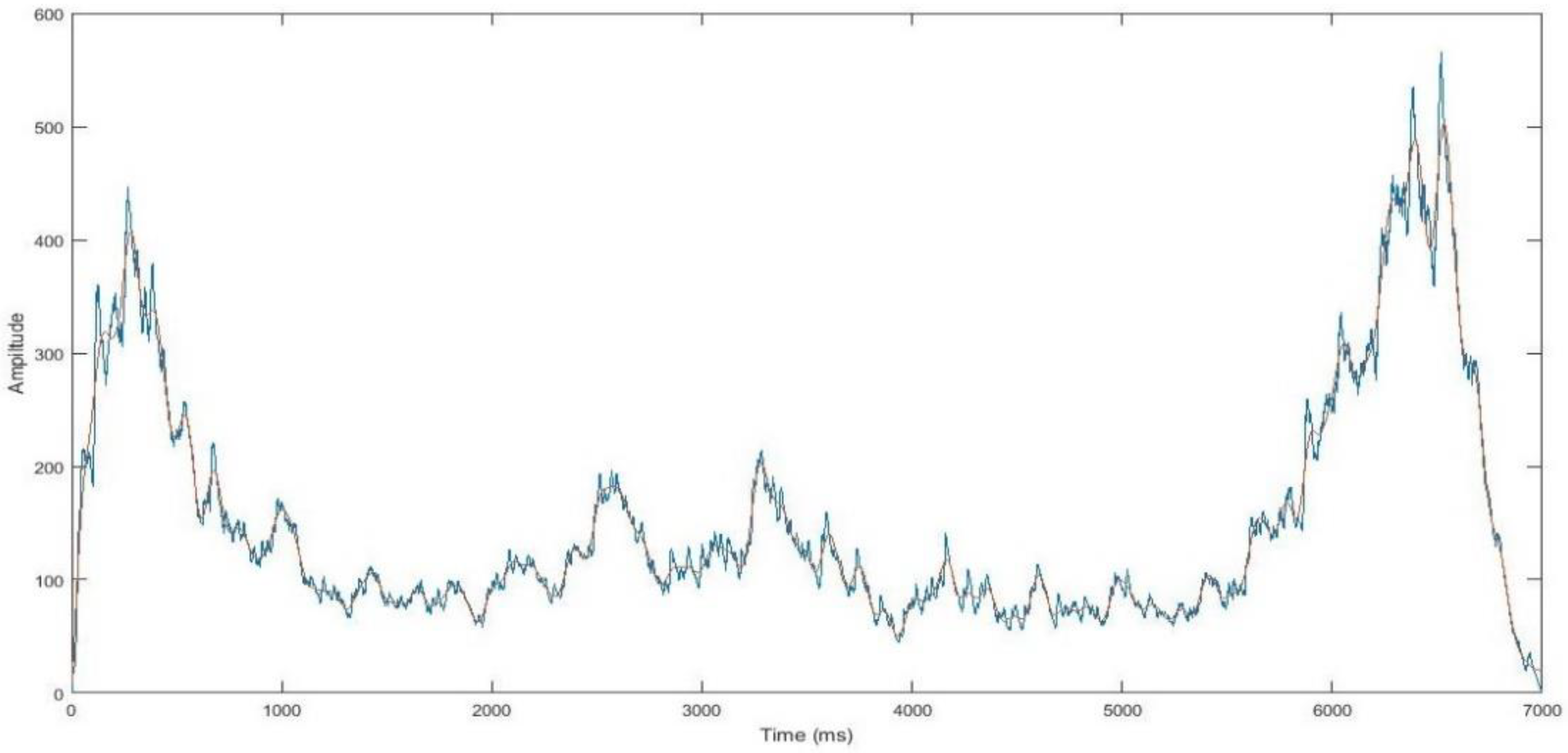
After collecting the raw SEMG signals with different loads as shown in Figure 7, Figure 8 and Figure 9. The amplitude of the SEMG signals for Subject C with a 3 kg load has been selected as reference amplitude of the SEMG signals in this experiment as shown in Figure 10. After converting the SEMG signal to the frequency domain using the Fast Fourier transform (FFT) as shown in Figure 11, one can observe the power of the SEMG signal below 10 Hz. After determining the cutoff frequency, the SEMG signal is passed through a fifth-order Butterworth low-pass filter with a cut off frequency of 10 Hz and the smooth signal is shown in Figure 12.

3.2. SEMG Feature Extraction

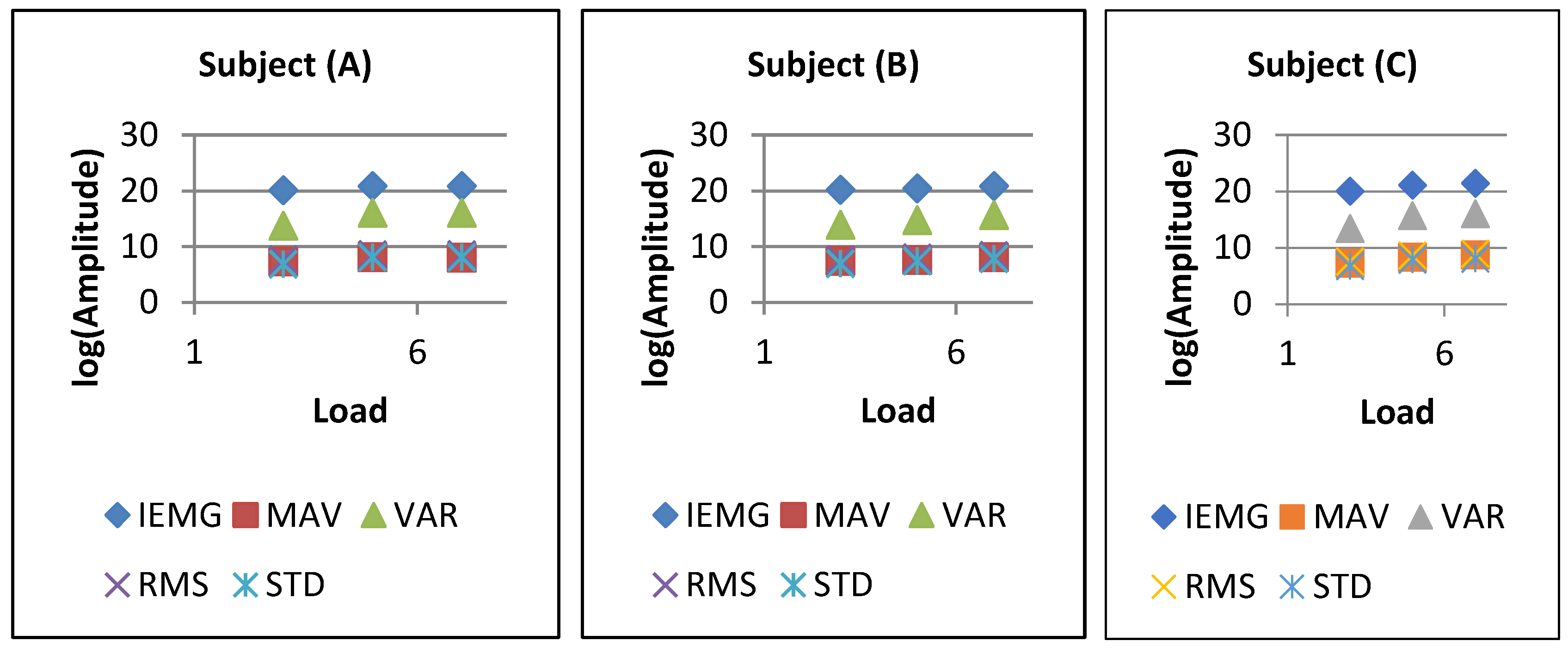
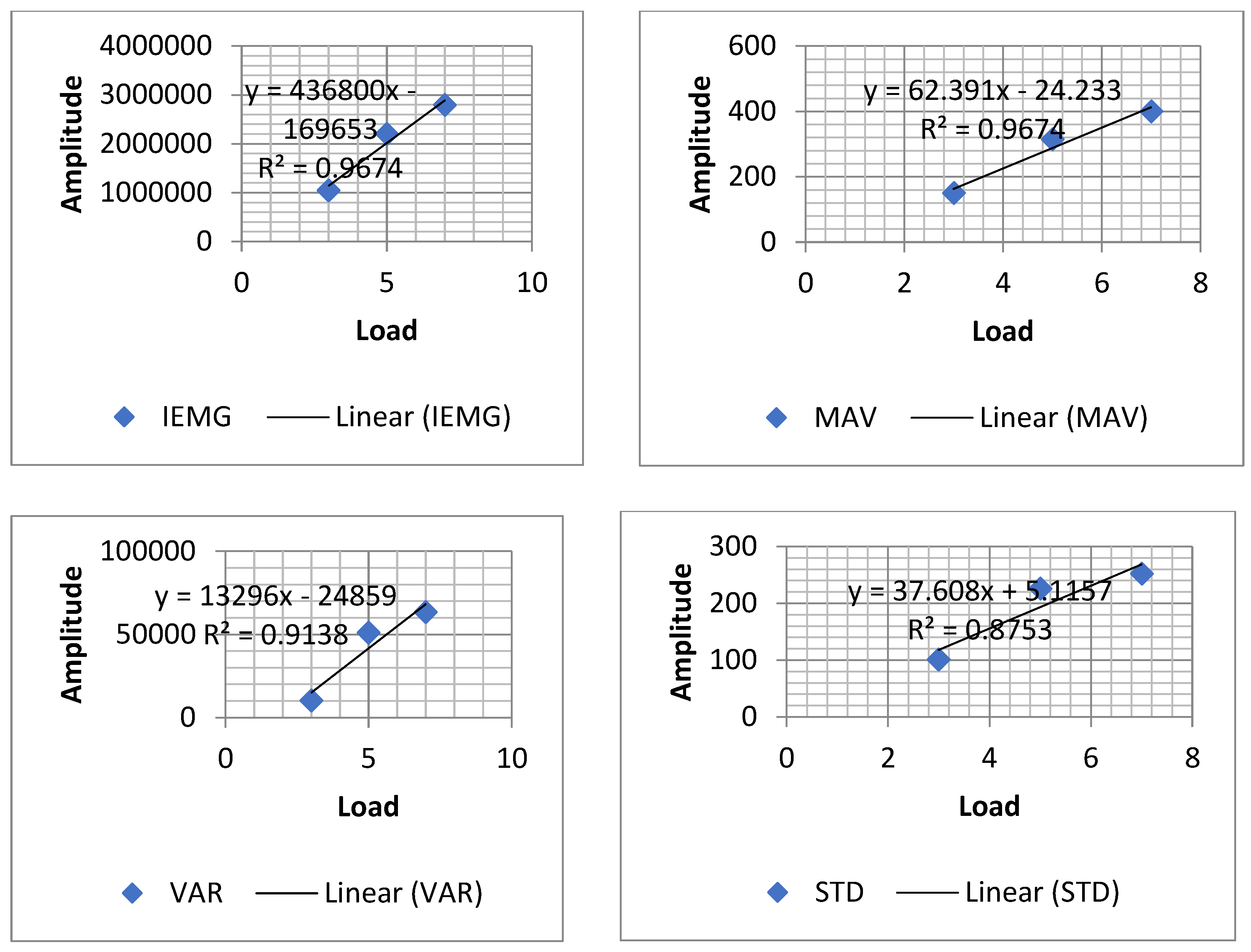
The time domain features analyze the relationship between the amplitude of the SEMG signal and load during the contraction of the bicep muscle. The SEMG signals were collected in the time domain with three various loads and three subjects in order to estimate the relationship between amplitude of the SEMG signal and the load. The smoothed signals for three subjects with 3 kg, 5 kg and 7 kg load go into the feature extraction process. The statistical features were selected IEMG, MAV, VAR, STD and RMS. The average value of five-time domain features is shown in

Table 2. Average values of five time domain features with three loads.

Subject	Load	IEMG	MAV	VAR	RMS	STD
A	3	1,093,437	156.183	12746.67	192.7121	112.9011
	5	1,760,043	251.3988	66570.16	360.2249	255.308
	7	1,822,112	260.2645	65182.16	364.5689	258.0119
B	3	1,135,594	162.2045	14573.65	202.1927	120.7214
	5	1,326,611	189.4888	25931.63	248.6643	161.033
	7	1,792,779	256.0747	47465.66	336.204	217.8661
C	3	1,048,218	149.724	10311.8	180.9078	101.547
	5	2,199,400	314.1551	51050.46	386.9581	225.9435
	7	2,795,416	399.2881	63493.9	472.1396	251.9799

. We can observe the values of the feature in the time domain for the SEMG signal changes according to the change of each load. That means when the load increases, the value of the feature in the time domain for the SEMG signal also increases, or in other words, the subject consumed more force when lifting his right hand with increasing load. As can be observed in Figure 13, the relationship of the five-time domain features was done as logarithm amplitude for the three subjects with three loads.

This research has chosen Subject C to create the model nerve signal for the bicep muscle. As can be observed in Figure 14, the fit linear model shows the relationship between amplitude SEMG signal and loads for Subject C of five time domain features (IEMG, MAV, VAR, RMS and STD) by using regression analysis with R-squared value. Based on the regression analysis, the better-fit model is the one with a higher R-squared or has a R-squared close to 1.00. Based on the result as shown in

Table 3. Mathematical fit linear model for five features.

Feature	Equation	$\mathbf{R}-\mathbf{Square}({\mathit{R}}^2)$
IEMG	y = 436800x − 169653	0.9674
MAV	y = 62.391x − 24.233	0.9674
VAR	y = 13296x − 24859	0.9138
RMS	y = 72.808x − 17.371	0.9457
STD	y = 37.608x + 5.1157	0.8753

, IEMG and MAV have the same R-squared value that is equal to 0.9674. This result means two approaches to model the relationship between amplitude SEMG signal and load. Table 3; shows all equations as fit linear model for five features (where x is the load (i.e., 3, 5 or 7 kg)). This research had chosen MAV as the reference feature to estimate the bicep muscle force that will be used in building modeling nerve signal for bicep muscle.

The bicep muscle force can be estimated by using Equation (7): [5,6].

y = 62.391x − 24.233

(7)

$$\begin{gathered} \mathrm{By}\mathrm{comparing}\mathrm{the}\mathrm{y}\mathrm{with}Amp\mathrm{and}\mathrm{x}\mathrm{with}L, \\ Amp=62.391L-24.233 \end{gathered}$$

(8)

$$L=0.016Amp+0.388$$

(9)

where $L$ is the load and $Amp$ is the amplitude of the SEMG signal, this means when the average amplitude of the SEMG signal Amp is 163; the value of the load (L) is ~ 3 kg

By comparing F with L,

$$F_{load}=0.016Amp+0.388$$

(10)

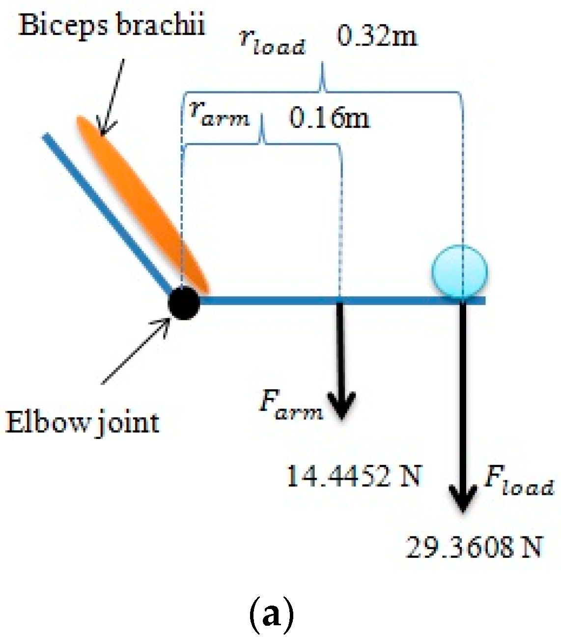
In Equation (10), $Amp$ is the amplitude of the SEMG signal and F is the average bicep muscle force. Note that this force should be multiplied with the gravity coefficient. This means that when $Amp$ is 163, then F is 29.3608 Newton.

3.3. Elbow Joint Torque Model

The torque of the elbow joint is the main idea for modeling the nerve signal for the bicep muscle; it will be used as input data in ANN. The data is collected for elbow joint torque when the subject started lifting the right hand from angle ${\theta }_{\mathrm{ej}}=0°$ to ${\theta }_{\mathrm{ej}}=90°$, which refers to elbow joint without movement of the shoulder joint with an increment of 0.03° in flexion elbow joint and decrement of 0.0225° in the extension elbow joint. Each increment and decrement in the angle are aligned with the sample number of the SEMG signal. The torque for the elbow joint is determined by using the standard torque Equation (11) [2].

$$\tau =\left(r_{load}{F}_{load}\right)+\left(r_{arm}{F}_{arm}\right)\cos \theta$$

(11)

where $r_{load}$ is the distance from the elbow joint to the load, $F_{load}$ is known as in Equation (10), $F_{arm}$ is the force due to the mass of the lower arm and $r_{arm}$ is the distance from the elbow joint to the center of mass of the lower arm which is half of $r_{load}$.

The segment mass can calculate by Equation (12) [18].

$$m_{seg}=p_i{m}_{total}$$

(12)

where $m_{seg}$ is segment mass, $p_i$ is a percentage segment mass from the table and $m_{total}$ is the total body mass.

The segment length can be calculated by Equation (13) [18].

$$l_{seg}=p_i/l_{total}$$

(13)

where l_seg is segment length, $p_i$ is a percentage segment length from the table, and $l_{total}$ is the body length.

The mass of the lower arm (forearm and hand) can be calculated by Equation (14).

$$M_{arm}=P_i{M}_{total}$$

(14)

where $M_{arm}$ is the mass lower arm, $M_{total}$ is the total body mass, $P_i$ is segment mass from anthropometric

Table 4. Normalized mass and length of body segments [18].

Segment	Segment Mass/Total Body Mass	Center of Mass/Segment Length		Density (kg/L)
		Proximal	Distal
Hand	0.006	0.506	0.494	1.16
Forearm	0.016	0.430	0.570	1.13
Upper Arm	0.028	0.436	0.564	1.07
Forearm and Hand	0.022	0.682	0.318	1.14
Total Arm	0.050	0.530	0.470	1.11
Head and Neck	0.081	1.000	—	1.11

. Which can be used to estimate the segment mass and segment length for different body parts.

The mass of subject C is 67 kg, $P_i$ equal 0.022 for forearm and hand then the $M_{arm}$ for Subject C is equal 1.474 kg. $F_{arm}$ is equal to $M_{arm}$ multiplied with gravity, this means the $F_{arm}$ is 14.4452 Newton. $r_{load}$ is 0.32m from elbow joint to load, $r_{arm}$ is 0.160 m half of $r_{load}$. This research will rewrite the torque equation in another form as shown in Equation (15).

$$\tau =\left(r_{load}\left(\left(0.016Amp+0.388\right)g\right)\right)+\left((r_{load}/2)\left(\left(P_i{M}_{total}\right)g\right)\right)\cos \theta$$

(15)

As can be observed in Figure 15a, the resistance forces are $F_{load}$ and $F_{arm}$, and distance from elbow joint $r_{load}$ and $r_{arm}$. Figure 15b shows the result of the torque for Subject C with three loads.

3.4. Artificial Neural Network

The artificial neural network (ANN) is a nonlinear model used in this research to model the SEMG signal with three loads 3 kg, 5 kg and 7 kg, since the SEMG signal is nonlinear. A multilayer perceptron (MLP) is a feed forward neural network consists of multiple layers with back-propagation algorithm technique to minimize the errors and supervised learning [19,20,21]. This research designed the ANN with MATLAB R2015a, and has chosen MLP with a Lavenberg–Marquardt training back-propagation algorithm, which can be used to enhance different area of research as in [22,23,24]. Several designs were tested in this research to choose the good neural network design, with the number of neurons from 10 to 60 in steps of 10. The neural network was trained on the data size of 7000 samples by dividing the data into three sets (i.e., 70% for training, 15% for validation and 15% for testing).

The MLP for modeling the nerve signal for the bicep muscle has three layers. The input layer consists of two nodes, which is denoted as A that represents the angle of movement of the forearm and represents the torque. Hidden layers consist of one layer with a number of neurons from 10 to 60 in steps of 10 to get the best performance. The output layer consists of one node, which is denoted as S to represent the SEMG signal. The mathematical representation of the neural network is:

$$y=f\left(w^{l}x+b^l\right)$$

(16)

$$h=f\left(w^{1}T+b^1\right)$$

$$\left[h_i\right]=f\left(\left[\begin{array}{c}\begin{array}{cc}{A}_1& A_2\begin{array}{cc}\dots & A_N\end{array}\end{array}\\ \begin{array}{cc}{\tau }_1& {\tau }_2\end{array}\begin{array}{cc}\cdots & {\tau }_N\end{array}\end{array}\right]\times \left[\begin{array}{c}\begin{array}{cc}{w}_{11}& w_{12}\end{array}\\ \begin{array}{cc}{w}_{21}& w_{22}\end{array}\\ \begin{array}{cc}⋮& ⋮\end{array}\\ \begin{array}{cc}{w}_{N1}& w_{N2}\end{array}\end{array}\right]+\left[\begin{array}{c}{b}_1\\ b_2\\ ⋮\\ b_N\end{array}\right]\right)$$

$$S=f\left(w^{2}h+b^2\right)$$

where $l$ is the number layer, the input ($\tau$, $A$) represented with an $m\times n$ matrix $T$, f used to represent an activation function in hidden layer of network is tan-sigmoid transfer function $\frac{e^n-e^{-n}}{e^n+e^{-n}}$ and in output layer is linear transfer function S = h. N used to represent the length signal which is equal 7000 samples, and b is bias in neural network. The network performed better with more neurons in the hidden layer as shown in

Table 5. Summary of the neural network results for three loads.

Load	Hidden Neurons	MSE	R-Square
3 kg	40	28.4723	0.9985
	50	1.8598	0.99991
	60	1.145	0.99993
5 kg	40	25.4304	0.99976
	50	17.896	0.99982
	60	1.3659	0.99999
7 kg	40	22.4425	0.99998
	50	3.5997	0.99997
	60	1.4238	0.99999

.

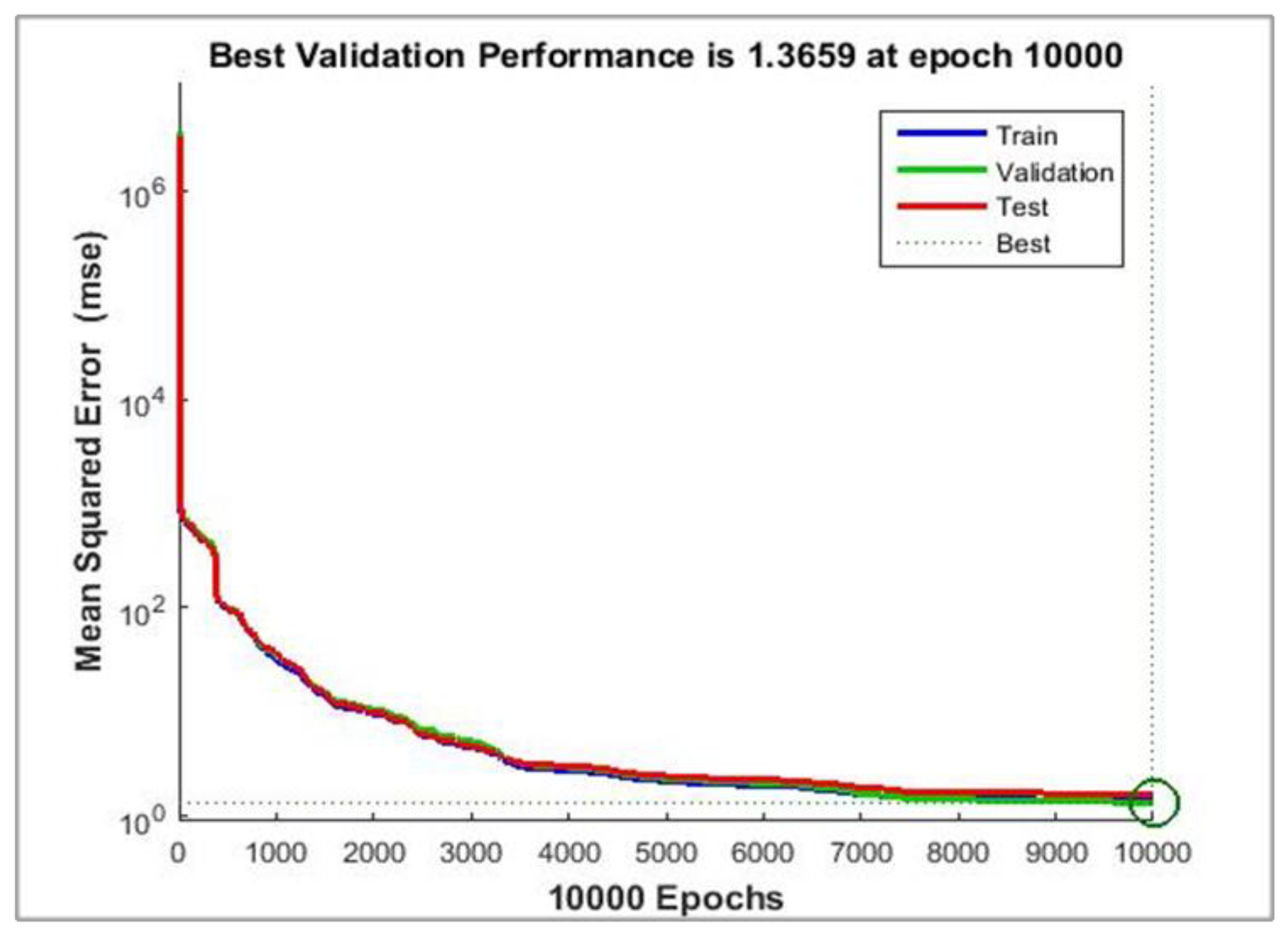
3.4.1. Resulting Model for Subject C with 5 Kg Load

The network with 60 neurons in the hidden layer is better network for 5 kg as shown in Figure 16 with the best validation performance of 1.3659 at epoch 10000. In this model, the regression result for training, testing and validation is 0.99999, which give an approximately optimal value for this model as shown in Figure 17. Figure 18 compares the prediction of the SEMG signal from the trained network and actual SEMG signal. The prediction of the SEMG signal has a good agreement with the nature of the actual SEMG signal.

3.4.2. Resulting Model for Subject C with 7 Kg Load

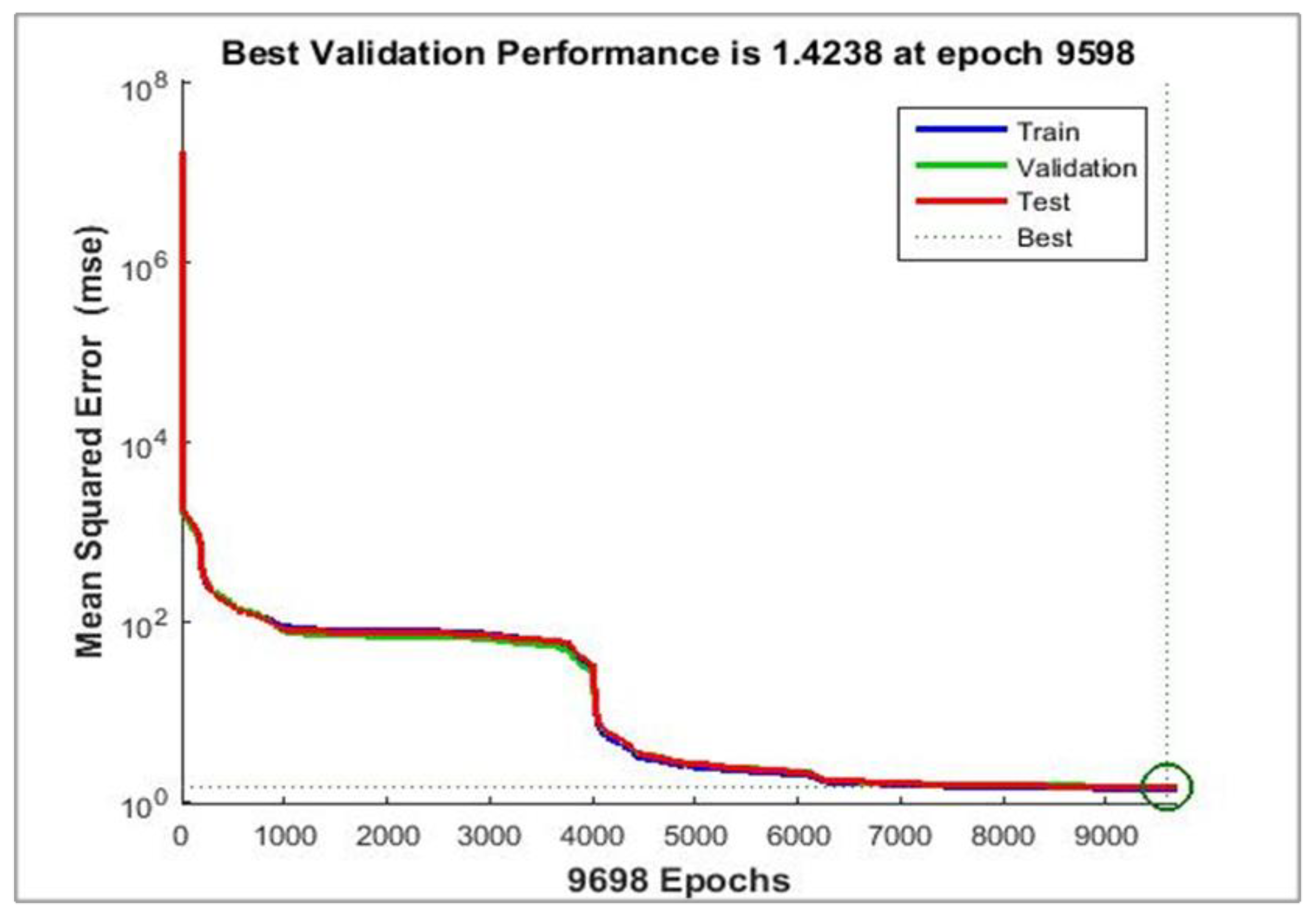
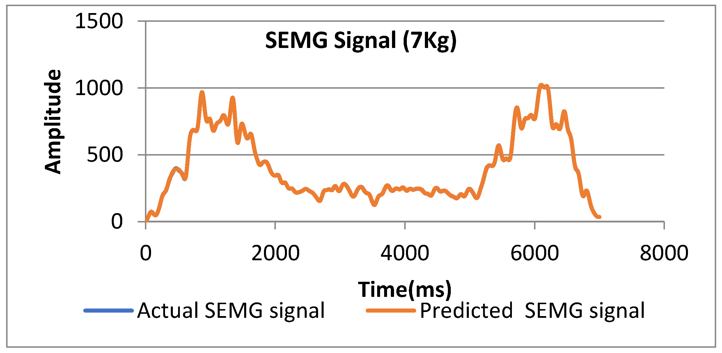
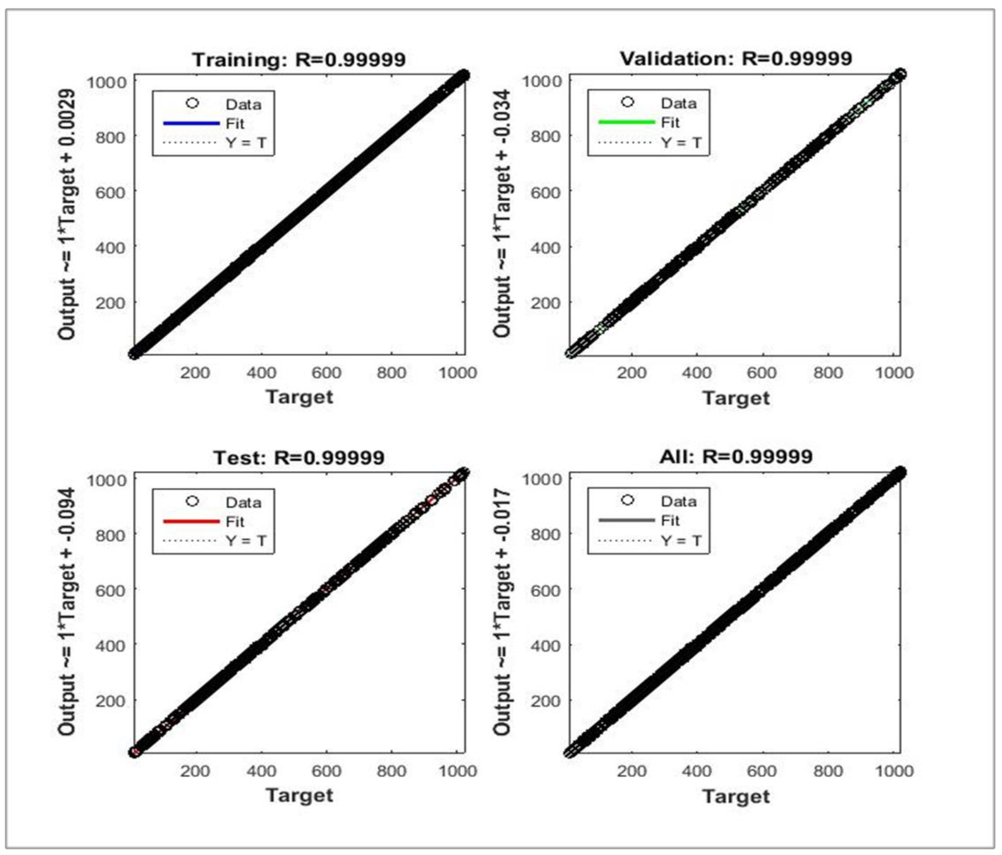
The network with 60 neurons in the hidden layer is a better network for the 7 kg load as shown in Figure 19 with the best validation performance of 1.4238 at epoch 9598. In this model, the regression result for training, testing and validation is 0.99999, which give an approximately optimal value for this model as shown in Figure 20. Figure 21 the compares the prediction of the SEMG signal from the trained network and actual SEMG signal. The prediction SEMG signal has a good agreement with the nature of the actual SEMG signal.

4. Conclusions

The surface electromyography (SEMG) is one of the bioelectrical signals for identifying muscular and nervous diseases. Studies show that several cases of nerve diseases lead to muscular dystrophy which, in turn, requires physiotherapy or even external electrical signals.

The SEMG signal is becoming more important in various applications, in this research; the SEMG signal is acquired from healthy subjects with three loads during dynamic contraction to model this signal that can be used to stimulate the muscle by electrodes to improve the possibility of movement in the human arm muscles. This was achieved using equipment developed to monitor and recode the SEMG signal. The signal was digitally filtered and used to estimate the average bicep muscle force by extracting five-time domain features. The model SEMG signal was achieved by using elbow joint torque for training the artificial neural network (ANN) with a different number of hidden neurons in order to optimize the network performance.

Based on the results, it can be concluded that the ANN model with two nodes at the input layer and 60 hidden neurons for three loads 3 kg, 5 kg and 7 kg produce MSE of 1.145, 1.3659 and 1.4238 and average regression of 0.99993, 0.99999 and 0.99999 for the SEMG signal with 5 kg and 7 kg. It is a good performance result as it shows that this neural network model can clearly represent the relationship between elbow joint torque and SEMG signals. The R-squared value determined the correlation between the SEMG amplitude with the loads. MAV was chosen as the reference feature for estimation of the bicep muscle force because of its R-squared value equal to 0.9674. By referring to the MAV, the linear equation obtained from the correlation was used for estimation of the bicep muscle force in the elbow joint torque.