The Improved Adaptive Silence Period Algorithm over Time-Variant Channels in the Cognitive Radio System


Information Science and Technology College, Dalian Maritime University, Dalian 116026, China
*
Author to whom correspondence should be addressed.
Future Internet 2018, 10(2), 12; https://doi.org/10.3390/fi10020012
Submission received: 28 November 2017
/
Revised: 24 January 2018
/
Accepted: 24 January 2018
/
Published: 29 January 2018
Abstract
:In the field of cognitive radio spectrum sensing, the adaptive silence period management mechanism (ASPM) has improved the problem of the low time-resource utilization rate of the traditional silence period management mechanism (TSPM). However, in the case of the low signal-to-noise ratio (SNR), the ASPM algorithm will increase the probability of missed detection for the primary user (PU). Focusing on this problem, this paper proposes an improved adaptive silence period management (IA-SPM) algorithm which can adaptively adjust the sensing parameters of the current period in combination with the feedback information from the data communication with the sensing results of the previous period. The feedback information in the channel is achieved with frequency resources rather than time resources in order to adapt to the parameter change in the time-varying channel. The Monte Carlo simulation results show that the detection probability of the IA-SPM is 10–15% higher than that of the ASPM under low SNR conditions.
1. Introduction
Cognitive radio (CR) has attracted considerable attention for its ability to maximize the rate of usage of limited spectrum resources [1,2,3]. The essence of the CR concept is opportunistic spectrum sharing [4]. Specifically speaking, this technology allows non-licensed users (secondary users, SUs) to opportunistically use primary users’ (PUs) frequency band resources for data transmission while the PUs are idle. These spectrum resources that are used by SUs during a specific period of time are referred to as ‘spectrum holes’. So, the performance of CR depends highly on the successful detection of the corresponding spectrum holes.
In a traditional sensing process in CR, time is divided into fixed portions which are called time slots. Each time slot is divided into a small period of spectrum sensing (silence period) and a relatively long period of data transmission [5]. In the sensing period, SUs use various techniques to sense if the PUs are active or idle. This is the typical “listen-before-talk” paradigm [6].
In the literature, several types of spectrum sensing schemes have been proposed. When the PU’s signal waveform and channel noise properties are known a priori, the matched filter detector is optimal [7]. The cyclostationary feature detection method requires a priori knowledge about the cyclic frequencies of the PU signals [8]. The energy detection method is usually simple to implement since it does not require knowledge about the PU signal. However, it does require the knowledge of the involved noise variance. The above three common spectrum sensing technologies are classified into the first type of spectrum sensing algorithm because they need to know the signal and/or channel information. Because these three typical spectrum sensing techniques need to know signal and/or channel information, they are grouped into the same group.
The second group of detectors for spectrum sensing are based on eigenvalue properties of an estimated correlation matrix. Because the eigenvalue-based spectrum sensing techniques may operate without knowledge of the PU signal [8] and noise variance [4], they can be used in a totally blind manner. The current research results in this area include the maximum eigenvalue detector [9], the maximum–minimum eigenvalue detector [9], the decentralized eigenvalue algorithms [10], the sequential likelihood ratio test scheme [11], and so on. These algorithms may offer a remarkably improved performance for specific signal categories. However, this is done at the expense of simplicity.
Different complexity spectrum detection algorithms will bring different degrees of delay. This will affect the proportion of the silence period in a time slot. Because no data transmission takes place during the silence period, an excessive silence period will reduce the SU’s throughput. So the management algorithm of the silence period is one of the key issues to improve the efficiency of spectrum sensing and time utilization.
In order to reduce the spectrum sensing time, an optimization algorithm which combines energy detection and feature detection is proposed [12]. Since energy detection focuses only on the energy level of the channel, it requires only a relatively short period of time for spectrum sensing. This method, through the results of energy detection, can determine whether it is needed to start feature detection or not, so it can improve the time utilization rate on the basis of ensuring sufficient detection accuracy in the silent periods. In [13], a mechanism to reduce the length of the silent period is given. When the number of continuous energy detection alarms is higher than a certain preset value, the characteristic detection is triggered. The Markov analysis is used to study the decision threshold of the energy detection results. In [14], a method of spectrum sensing without the silence period is proposed in which the secondary user (SU) performs spectrum sensing for the primary users (PU) while carrying out the data transmission. In this algorithm, the detection node first uses the linear prediction method to estimate the signal characteristics of the SUs in the next period. Then, in the spectrum sensing, the result of subtracting the estimated value from the received signal is used as the judgment criterion to determine whether the PU exists or not. In [15], the authors add a feedback time slot in the center-based spectrum allocation algorithm architecture, so that the number of sampling points can be adjusted automatically according to the feedback information. However, in the case of low signal-to-noise ratio (SNR), it cannot guarantee the reliable transmission of the feedback information which allows for the possibility of over-regulation which will reduce the detection probability of the PU. At the same time, the introduction of the feedback time slot will also reduce the time utilization rate of the time resources to a certain extent.
Referring to the ideas on feedback information proposed in [15], we constructed a cognitive wireless communication system model with an additional signaling channel. The model utilizes additional frequency resources rather than time resources to feedback the state information of the data transmission which can characterize the time-varying channel characteristics in the data transmission. So, on this basis, an improved adaptive silence period management (IA-SPM) algorithm is proposed. The algorithm combines the results of the previous perception period with the data channel communication result feedback from the signaling channel to adaptively adjust the relevant parameters to be used in the current sensing period. The signaling channel can not only reduce the interference of noise, but it can also ensure the reliability of the transmission through coding error correction. Meanwhile, we used the discrete Markov analysis method to construct a mathematical simulation model of the system and analyze the detection probability of the proposed algorithm. As a result, in the case of low SNR, the detection probability of our algorithm was 10–15% higher than that of the algorithm proposed in [16].
2. The Silence Period Management (SPM) Algorithm
In the cognitive radio network, the SU carries on the spectrum sensing to the PU’s frequency band to find the free band and wait for access [17]. In the process of spectrum sensing, the SU receives signals not only from PUs and noise, but also from other SUs. In order to avoid interference in the detection results, when the SU performs spectrum sensing, all SUs in the system need to stop any transmitting activities. This time in the periodic window is called the silence period. In order to enhance the time utilization rate, the length of the silence period needs to be reasonably optimized.
Figure 1a is a schematic diagram of the slot division scheme in the traditional silent period algorithm. The sensing period is divided into the silent period and the sensing interval. The SU determines whether the data can be transmitted during the sensing interval based on the sensing results of the silence period. Figure 1b is a schematic diagram of the slot division scheme in the adaptive silence period algorithm. One of the most significant changes is the addition of a feedback slot at the end of each sensing period.
As shown in the figure, is the sensing period, is the time length of the silence period, and is the time length of the data transmission. In general, the parameter is keeps constant. Additionally, in the traditional sensing period algorithm, is equal within each sensing period. However, in the adaptive sensing period algorithm, is different in each sensing period.
3. System Modeling
In a wireless communication system, the signal power not only decreases with increasing propagation distance, but it is also affected by the additional fading caused by a variety of obstacles or complex terrain. At the same time, this additional fading will change randomly due to the movement of the mobile station and the change of the channel environment. The time-varying characteristic of this wireless channel will cause the received signal to be distorted, with the waveform broadened and overlapping, which affects the communication quality of the channel [18]. In severe cases, it may lead to communication abnormalities.
The traditional adaptive silence management algorithm uses the shared data band to transmit feedback information. When the data band is affected by the environment and causes a sharp decline in the signal, the system performance of the scheme deteriorates significantly due to the fact that the SU cannot obtain the feedback information reliably.
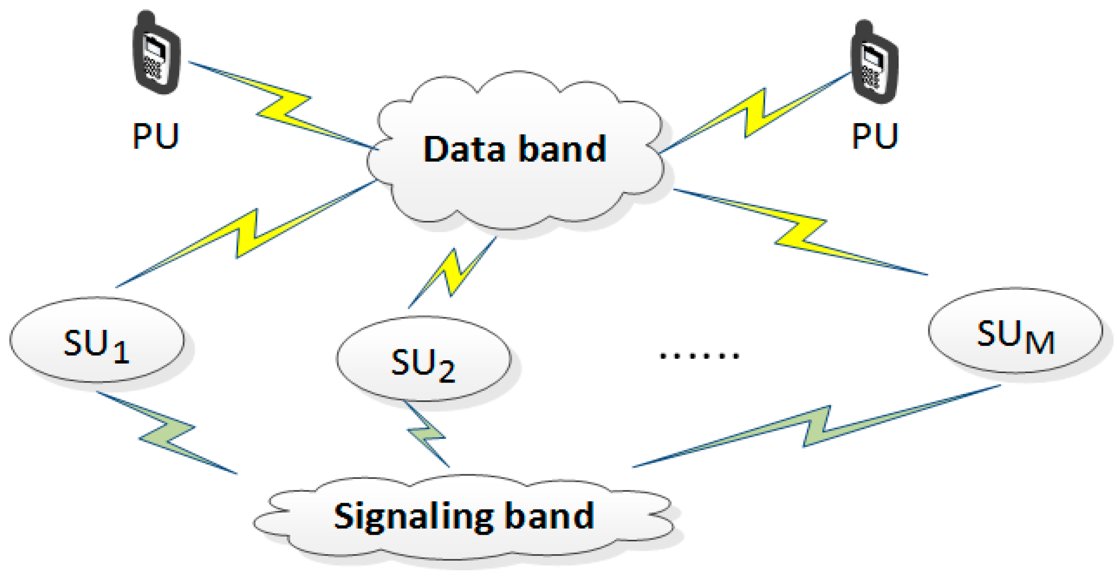
Considering that the small-scale fading in a wireless channel usually has frequency selectivity, we made a decision to construct a cognitive wireless communication system with an additional signaling channel (CWCS-ASC). The corresponding system model is shown in Figure 2. By selecting the specific frequency band outside the spectrum of the data channel as the signaling channel, adding the signaling channel not only avoids the influence of the PU on the signal transmission, but also enables the SU to divide the time into non-overlapping frames, and then divide the frames into non-overlapping channels. Additionally, the users will have one-to-one correspondence according to the time slot, in order to distinguish users from different addresses of the signal, thus completing the multiple access. Furthermore, opening additional signaling channels can increase the additional transmission power and through the error correction coding to reduce the noise interference, the system can still guarantee the reliable transmission of feedback information even when the data band suffers a great fading.
The information interaction sequence diagram for the CWCS-ASC system is shown in Figure 3. The SU decides whether to transmit data by the data band based on the perceived results of the current silent period and their own communication needs. The time window used to transmit data is defined as the data transmission period, whose length of time needs to be less than the sensing interval . The difference between the sensing interval and the data transmission period is defined as the free period. The longer the silence period, the higher the reliability of the detection, the lower the utilization rate of the band, and the smaller the throughput of the cognitive user [19]. The presence of the free period ensures that the data transmission from the SU does not interfere with the spectrum sensing in the next sensing period.
In order to avoid communication conflicts, after obtaining the sensing result, the SU will use the signaling slot in the signaling band to transmit interactive information which is used to coordinate the allocation algorithm among SUs. In addition, after a certain secondary user (SU1) sends the business data, the other SUs in the region will generate feedback information based on the result of the received signals. Then they send the feedback information to the SU1 via the feedback slot in the signaling band. The SU1 can estimate the channel characteristics based on the feedback information obtained, thereby reasonably adjusting the configuration parameters for the next silent period.
4. Mathematical Modelling and the IA-SPM Algorithm
In cognitive radio systems, SUs must always check whether a frequency band is being occupied by the PU. The PU has the highest priority. If a certain SU discovers that the PU appears during the transmission of the data, the SU will immediately stop the data transmission process. The PU status is detected by the SU in each sensing period as either in an active state or an idle state.
4.1. The IA-SPM Model Based on the Markov Chain
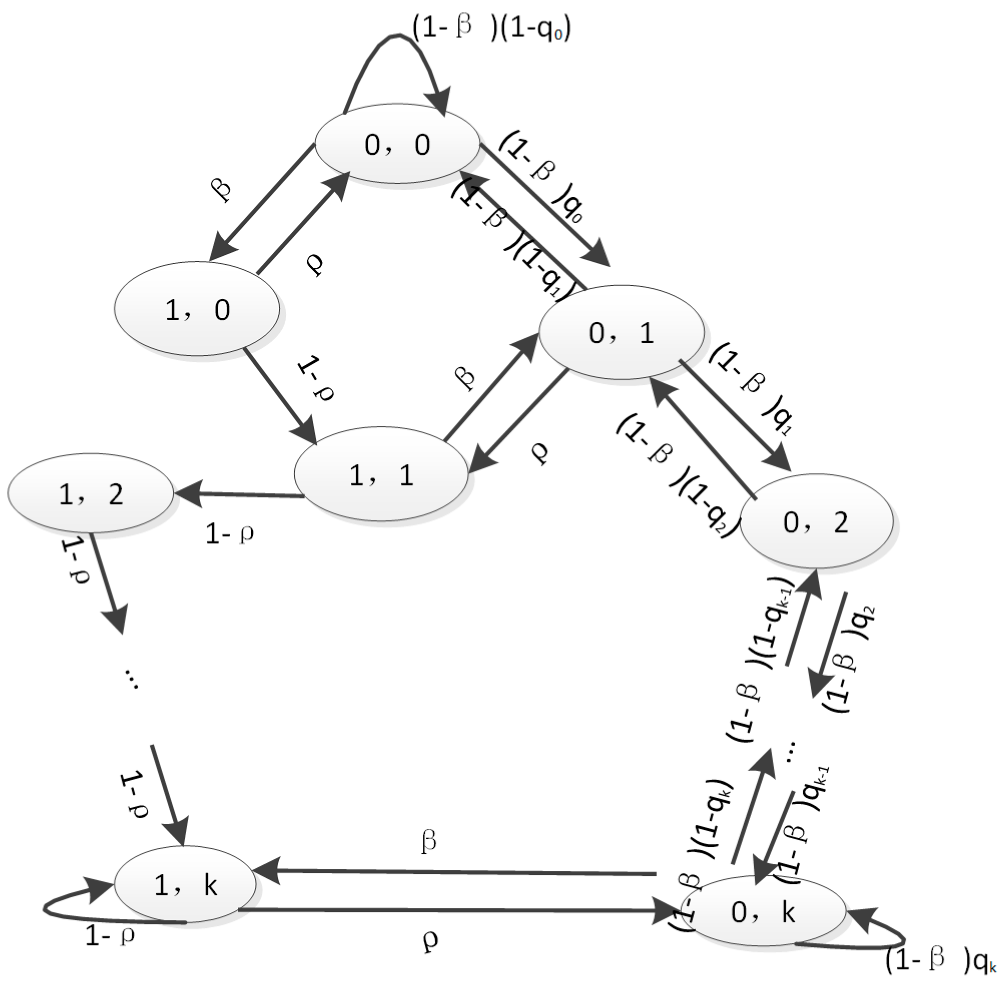
Assuming that the cognitive user detects the channel at the beginning of each sensing period, the system state can be modeled as a discrete time Markov chain. The system state is represented by , where indicates the status of the authorized user. When , it indicates that the PU exist. Otherwise, the PU does not exist. indicates the serial number of the silent period. and , respectively, represent the false alarm probability of system states and . Since the false alarm probability and false dismissal probability is a random process, the SU’s detection process satisfies the Markovian nature. It has the properties
We define the K-step transition probability as .
Assuming that the probability of using the frequency band by the PU is and the probability of releasing the frequency band by the PU is , the state transition of the system can be obtained by the state transition diagram which is shown in Figure 4. In this system model, denotes the stationary probability of the state .
The stability probability of each state can be obtained by the above flow Equations (2)–(7). The normalized equation can be expressed as
4.2. The IA-SPM Algorithm
The state equation is analyzed by the discrete Markov process, and the quantitative analysis of the system detection probability of the IA-SPM is obtained.
According to the state of the PU, when the SU sends the data, the signal stored in the frequency band can be represented by the formula
where k represents the sampling time, is the signal stored in the frequency band, indicates the signal transmitted by the PU, indicates the signal transmitted by the PU, and is the existence of a probabilistic problem. In order to facilitate the study, we assume that it is a single-carrier modulated, phase-modulated signal and that the channel it is passed through is an additive Gaussian white noise channel. indicates that the PU is in an idle state and indicates that the PU is in an active state. In order to reduce the complexity of the analysis, it is assumed that there is no channel noise. When the system is in the state, there is a conflict.
Assuming that and are random processes with a Gaussian distribution, their mean is 0 and their variance is and , respectively. For an SU that receives the signal, is a useful signal and is an interfering noise. So is defined as the signal-to-noise ratio, which represents the power ratio of the PU transmitting signal to the SU transmitting signal.
It is the key to how to adaptively adjust the parameters of the silent period under the condition that the sensing period is determined. The minimum length of the silence period is specified as and the maximum length is . The IA-SPM is divided into the following two conditions:
Condition 1: If an SU judges that the PU is not present based on the perceived result during the current silence period, it will send the data and then wait for the response from the receiver.
If the SU sender receives the feedback signal successfully, it is judged that the PU does not exist. So the self-detection time of the next period can be reduced. The sampling points are reduced by times, expressed by the formula
If the SU sender does not receive the feedback signal, it judges that the PU is present. Then the next period of self-detection time increases. So that the energy detection can be greater than the threshold, the number of sampling points is expanded by times, expressed by the formula
Condition 2: If an SU judges that the PU is present based on the perceived results during the current silence period, it will automatically increase the length of the silence until it is determined that the PU has disappeared.
Then, the silent period of the next sensing cycle remains unchanged until the SU judges that the PU does not exist. This will then go to Condition 1.
5. Simulation and Results Analysis
5.1. Simulation Model
In order to analyze the performance of the IA-SPM, the detection probability of the cognitive radio network is calculated.
Let be the number of samples in silence and be the selected detection threshold. The detection probability of the system can be expressed as [20]
where represents the power ratio between the PU signal and the SU signal. In this paper, it is named the SNR. It is well known that in the time-varying channel, the SNR is time-varying. In order to ensure that the study is not affected by other factors, we assume that the SNR is time varying in different periods and that the SNR is kept constant in the same period. The detection points have different energy-aware samples in different periods.
The state equilibrium equation of the Markov chain represented by the Equation (8) can be used to solve the detection probability
Assuming that each silence period is and the sensing period is , the signal will be sampled at the Nyquist sampling frequency . Then we can get the following relationship between the silence period and the number of samples per period
Since the impulse response of the fading channel is time-varying, the SNR of the channel varies randomly within a finite interval. Assuming that the SU uses the energy detection method for spectrum sensing and that the SUs do not know the current SNR, the threshold for energy detection should be represented by the equation
where is the false dismissal probability.
5.2. Results Analysis
In order to compare the detection probability of the IA-SPM with the TSPM and the ASPM, the Monte Carlo simulation is used to analyze the models. In the following experiment, we did the simulation 1000 times in each period
In this paper, the efficiency of the IA-SPM is determined by the average number of samples. The higher the number of samples, the higher the cost of the IA-SPM, the larger the parameter , and the higher the linearity of the number of samples. Therefore, in order to jointly optimize the number of samples and the probability of detection, we compare the selection of parameter . According to the detection probability of under different values, as shown below Figure 5.
It can be seen from the figure that both the detection probabilities of IA-SPM and ASPM are influenced by the parameter . The detection probabilities of these two algorithms showed a monotonically increasing trend with the increase of . However, when the value of exceeds a certain threshold, the detection probabilities of both algorithms tend to be stable. In addition, the maximum detection probability of IA-SPM algorithm is better than ASPM algorithm. Therefore, in the following experiment, we set the parameter and the SNR was used to simulate the channel’s time-varying characteristics within a certain range.
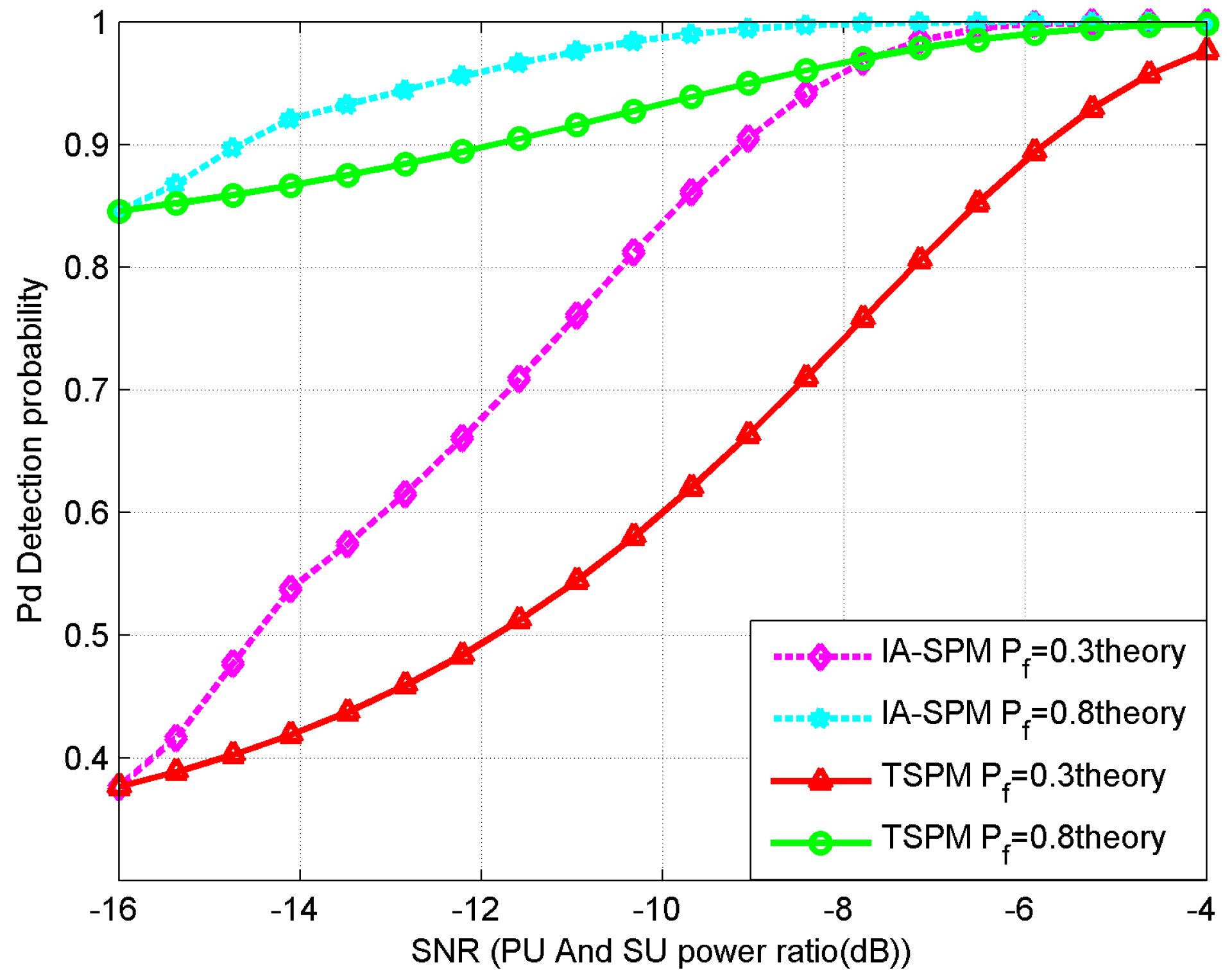
First, we compared the improvement of the IA-SPM algorithm with respect to the TSPM algorithm. The simulation results are shown in Figure 6.
We found that in any kind of detection algorithm the greater the SNR, the greater the detection probability; and the greater the false dismissal probability, the higher the probability of detection. At the same time, it can be clearly seen that the detection probability of the IA-SPM is superior to that of the TSPM under the same conditions.
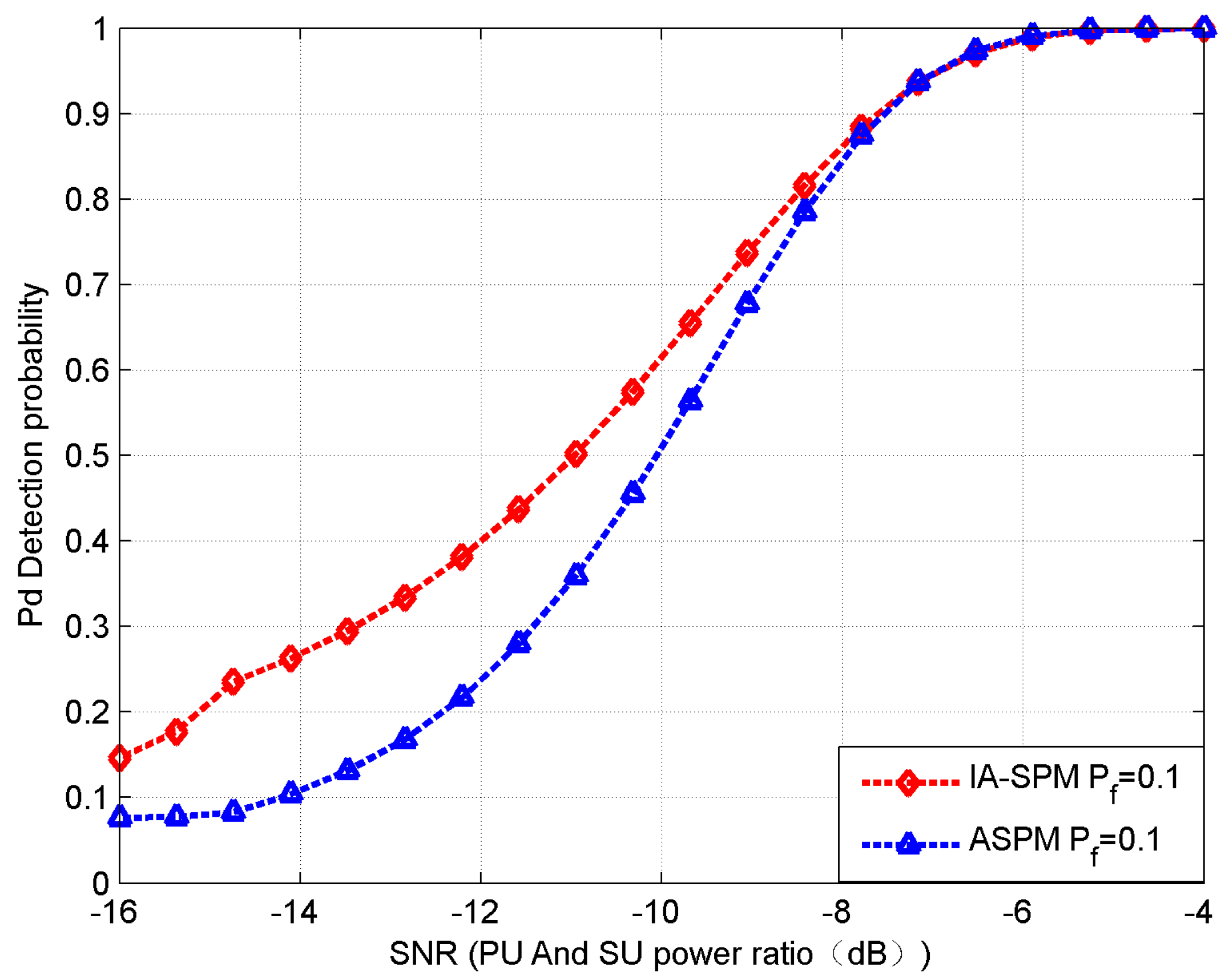
Then, we compared the detection probability of the IA-SPM algorithm with the ASPM algorithm under the same SNR conditions. The simulation results are shown in Figure 7.
As the result shows, the detection probability of the IA-SPM is better than that of the ASPM. Especially under low SNR conditions, the IA-SPM is better than the ASPM by 10–15%. With the increase of the SNR, the detection efficiency of the two algorithms tends to be consistent. This data shows that the IA-SPM is more suitable for time-varying channels.
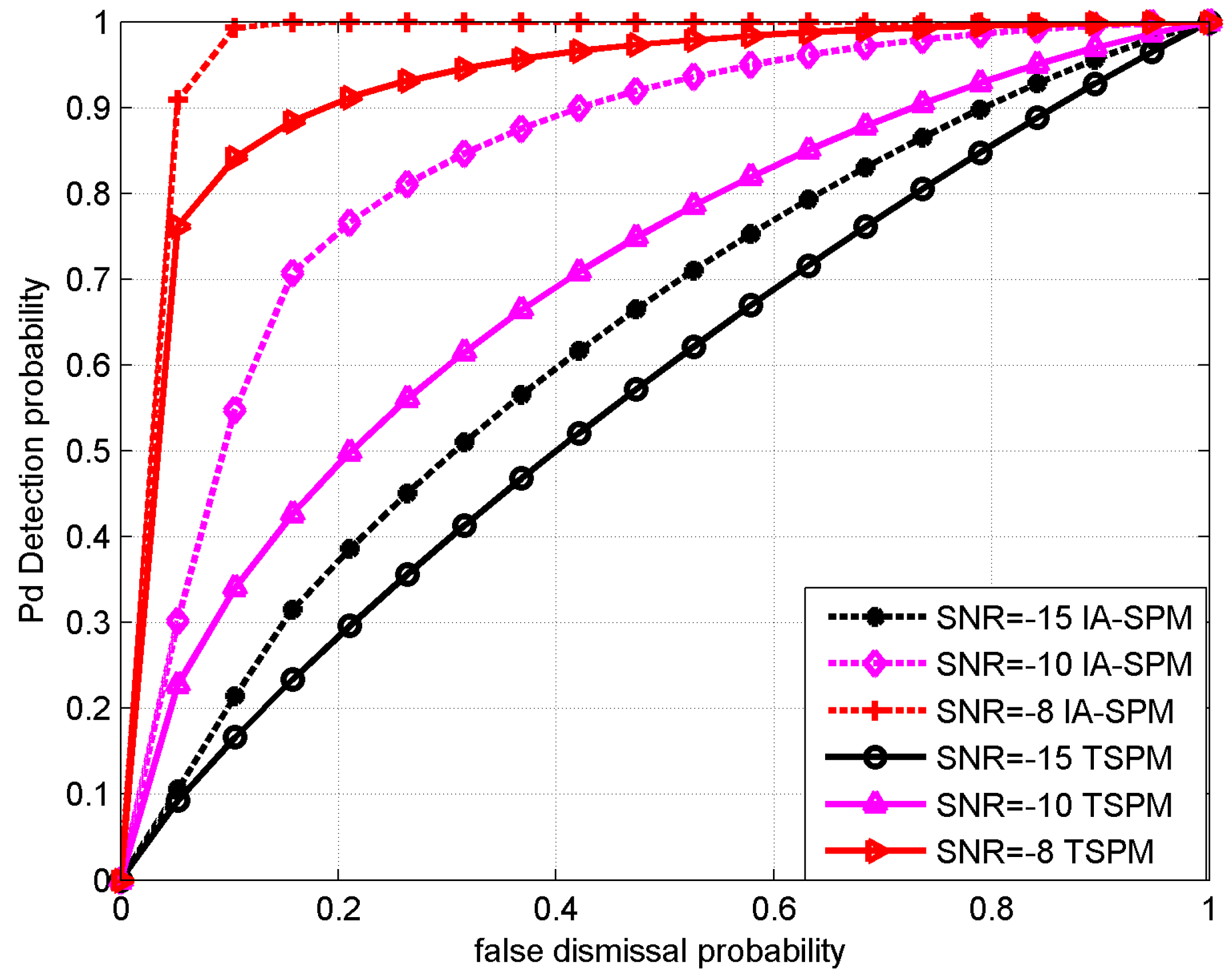
Finally, we set the SNR to be equal to −15, −10, and −8 dB. Under these three conditions, we compared the differences of the false dismissal probability between the IA-SPM algorithm and the TSPM algorithm. The simulation results are shown in Figure 8.
Through the above figures we can find that, in the same case, with the increase of the false dismissal probability, the probability of detection, and the SNR increase at the same time. So, we can see that the results of the IA-SPM are much higher than that of the TSPM.
6. Conclusions
For the issue of channel time-varying in wireless communication, we have established an IA-SPM communication model which carries out signaling transmission among SUs so that the SUs can obtain the feedback information through an additional spectrum. By setting additional signaling bands, on the one hand, the time efficiency of the data band can be improved, and on the other hand, channel interference to the feedback information can be avoided.
On this basis, we propose the IA-SPM algorithm which can adjust the parameters of spectrum sensing such as the length of the silence duration and the length of the transmission. The change of the parameters depends on the spectrum sensing results and the data transmission feedback information in the previous periods.
In the case of low SNR, this algorithm that makes the sampling points will not have a steep drop so the algorithm can better guarantee the detection performance in the time-varying channel environment. Simulation results show that the IA-SPM is 10–15% higher than the ASPM under low SNR conditions.
Acknowledgments
This work was supported by the Chinese National Science Foundation under grants 61501078, 61601078, and 61231006, the Fundamental Research Funds for the Central Universities under grant 3132016208.
Author Contributions
Jingbo Zhang designed the CSCS-ASC system model and the time sequence diagram of the system information interaction and organized the paper; Zhenyang Sun carried out the simulations and was responsible for the writing and editing of the manuscript; and Shufang Zhang supervised the work and contributed to the writing of the paper.
Conflicts of Interest
The authors declare no conflict of interest.
References
- Fantacci, R.; Marabissi, D. Cognitive Spectrum Sharing: An Enabling Wireless Communication Technology for a Wide Use of Smart Systems. Future Internet 2016, 8, 23. [Google Scholar] [CrossRef]
- Bayrakdar, M.E.; Atmaca, S.; Karahan, A. A slotted ALOHA-based cognitive radio network under capture effect in Rayleigh fading channels. Turkish J. Electr. Eng. Comput. Sci. 2016, 24, 1955–1966. [Google Scholar] [CrossRef]
- Chen, Y.; Zhou, H.; Kong, R.; Zhu, L.; Mao, H. Decentralized Blind Spectrum Selection in Cognitive Radio Networks Considering Handoff Cost. Future Internet 2017, 9, 10. [Google Scholar] [CrossRef]
- Tsinos, C.G.; Berberidis, K. Decentralized Adaptive Eigenvalue-Based Spectrum Sensing for Multiantenna Cognitive Radio Systems. IEEE Trans. Wirel. Commun. 2015, 14, 1703–1715. [Google Scholar] [CrossRef]
- Zhao, Y.; Hong, Z.; Wang, G.; Huang, J. High-Order Hidden Bivariate Markov Model: A Novel Approach on Spectrum Prediction. In Proceedings of the 25th International Conference on Computer Communication and Networks (ICCCN), Waikoloa, HI, USA, 1–4 August 2016; pp. 1–7. [Google Scholar]
- Politis, C.; Maleki, S.; Tsinos, C.G.; Liolis, K.P.; Chatzinotas, S.; Ottersten, B. Simultaneous Sensing and Transmission for Cognitive Radios With Imperfect Signal Cancellation. IEEE Trans. Wirel. Commun. 2017, 16, 5599–5615. [Google Scholar] [CrossRef]
- Ma, J.; Li, G.Y.; Juang, B.H. Signal processing in cognitive radio. Proc. IEEE 2009, 97, 805–823. [Google Scholar]
- Ainomae, A.; Bengtsson, M.; Trump, T. Distributed Largest Eigenvalue Based Spectrum Sensing using Diffusion LMS. IEEE Trans. Signal Inf. Process. Netw. 2017. [Google Scholar] [CrossRef]
- Zeng, Y.; Liang, Y.C. Eigenvalue-based spectrum sensing algorithms for cognitive radio. IEEE Trans. Commun. 2009, 57, 1784–1793. [Google Scholar] [CrossRef]
- Penna, F.; Stańczak, S. Decentralized Eigenvalue Algorithms for Distributed Signal Detection in Wireless Networks. IEEE Trans. Signal Process. 2015, 63, 427–440. [Google Scholar] [CrossRef]
- Renard, J.; Lampe, L.; Horlin, F. Sequential Likelihood Ratio Test for Cognitive Radios. IEEE Trans. Signal Process. 2016, 64, 6627–6639. [Google Scholar] [CrossRef]
- Cabric, D.; Mishra, S.M.; Brodersen, R.W. Implementation issues in spectrum sensing for cognitive radios. In Proceedings of the Thirty-Eighth Asilomar Conference on Signals, Systems and Computers, Pacific Grove, CA, USA, 7–10 November 2004; pp. 772–776. [Google Scholar]
- Jeon, W.S.; Jeong, D.G. An advanced quiet period management scheme for cognitive radio systems. IEEE Trans. Veh. Technol. 2010, 59, 1242–1256. [Google Scholar] [CrossRef]
- Song, Z.; Zhou, Z.; Sun, X.; Ye, Y. Nonquiet primary user detection scheme. In Proceedings of the 6th International ICST Conference on Communications and Networking in China, Harbin, China, 17–19 August 2011; pp. 473–477. [Google Scholar]
- Sun, X.; Zhou, Z.; Zou, W. Adaptive quiet period management scheme over time-variant channels in cognitive radio networks. J. Converg. Inf. Technol. 2011, 11, 284–290. [Google Scholar]
- Zheng, M.; Chen, L.; Liang, W.; Yu, H.; Wu, J. Energy-Efficiency Maximization for Cooperative Spectrum Sensing in Cognitive Sensor Networks. IEEE Trans. Green Commun. Netw. 2017, 1, 29–39. [Google Scholar] [CrossRef]
- Tadayon, N.; Aïssa, S. A Multichannel Spectrum Sensing Fusion Mechanism for Cognitive Radio Networks: Design and Application to IEEE 802.22 WRANs. IEEE Trans. Cognitive Commun. Netw. 2015, 1, 359–371. [Google Scholar] [CrossRef]
- Sun, X.; Djordjevic, I.B.; Neifeld, M.A. Secret Key Rates and Optimization of BB84 and Decoy State Protocols Over Time-Varying Free-Space Optical Channels. IEEE Photonics J. 2016, 8, 1–13. [Google Scholar] [CrossRef]
- Qin, Y.; Zhong, X.; Yang, Y.; Li, Y.; Li, L. Joint channel assignment and opportunistic routing for maximizing throughput in cognitive radio networks. In Proceedings of the 2014 IEEE Global Communications Conference, Austin, TX, USA, 8–12 December 2014; pp. 4592–4597. [Google Scholar]
- Cardenas-Juarez, M.; Pineda-Rico, U.; Stevens-Navarro, E.; Ghogho, M. Sensing-throughput optimization for cognitive radio networks under outage constraints and hard decision fusion. In Proceedings of the 2015 International Conference on Electronics, Communications and Computers (CONIELECOMP), Cholula, Mexico, 25–27 February 2015; pp. 80–86. [Google Scholar]
Figure 1.
The slot division scheme of the SPM algorithm (a) Traditional silence period; (b) Adaptive silence period.
Figure 1.
The slot division scheme of the SPM algorithm (a) Traditional silence period; (b) Adaptive silence period.
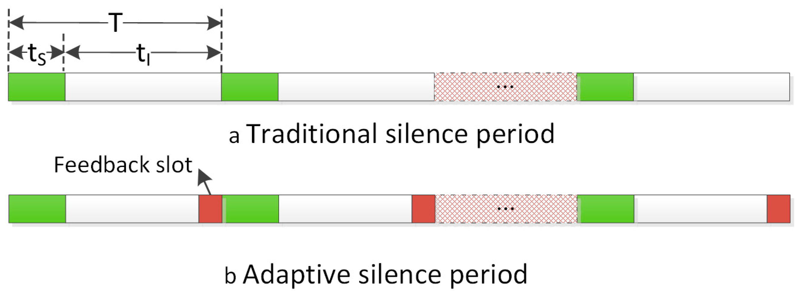
Figure 2.
The cognitive wireless communication system with an additional signaling channel (CSCS-ASC) system model.
Figure 2.
The cognitive wireless communication system with an additional signaling channel (CSCS-ASC) system model.

Figure 3.
The time sequence diagram of the system information interaction.
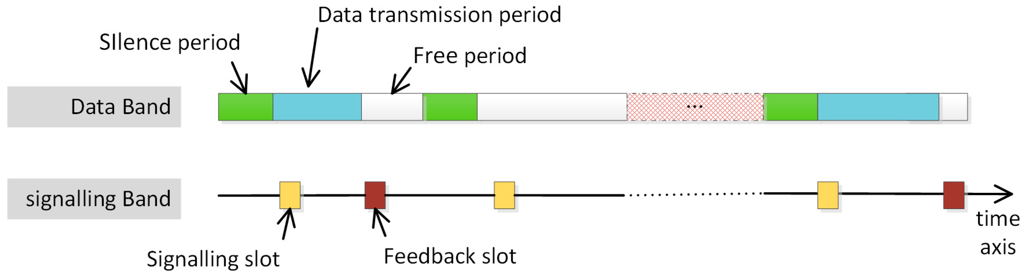
Figure 4.
The state transition equation.

Figure 5.
Comparison of the IA-SPM vs. the TSPM with different .
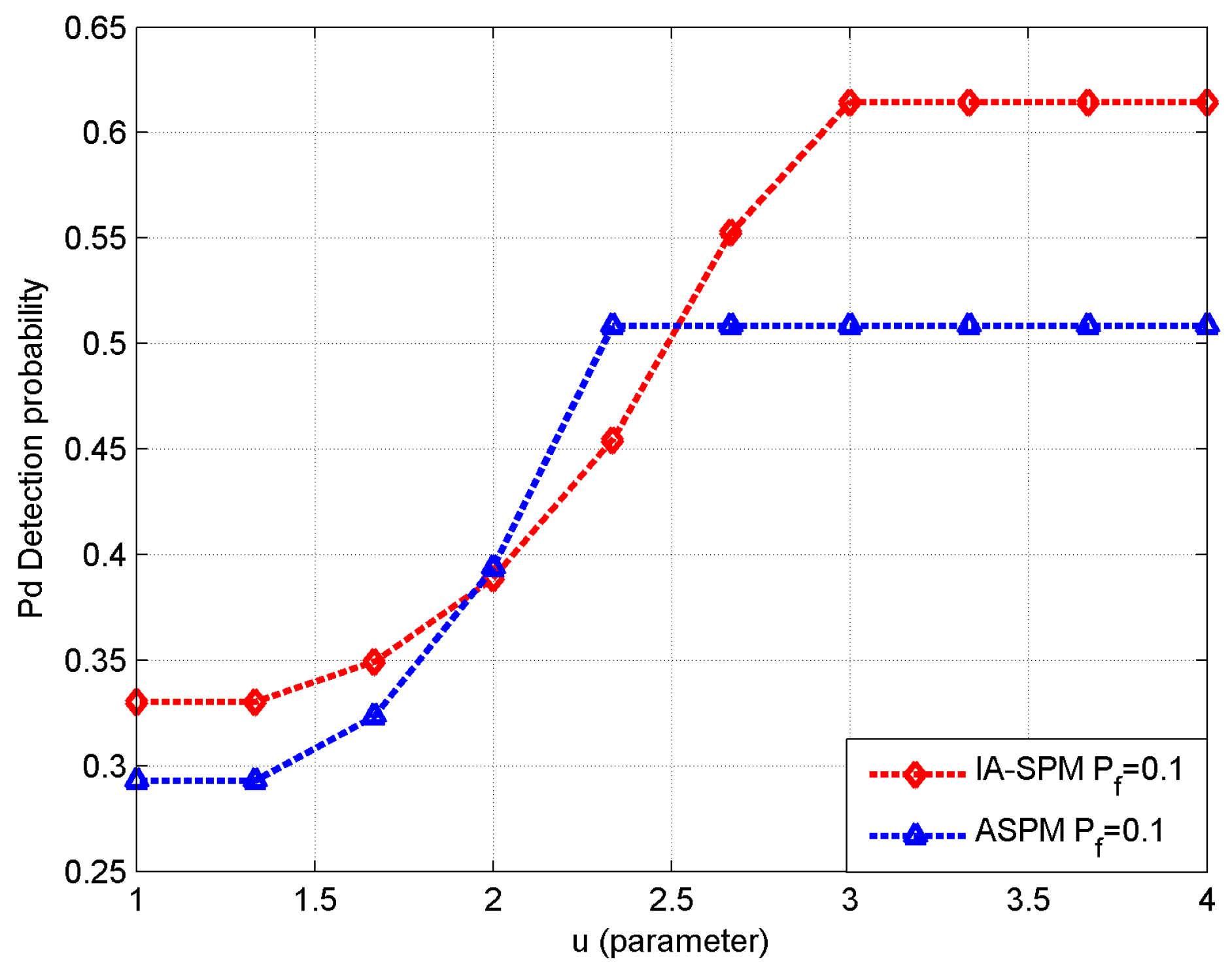
Figure 6.
Comparison of the IA-SPM vs. the TSPM with different false dismissal probabilities.

Figure 7.
The IA-SPM vs. the ASPM.

Figure 8.
Comparison of the IA-SPM vs. the TSPM at different SNR values.

© 2018 by the authors. Licensee MDPI, Basel, Switzerland. This article is an open access article distributed under the terms and conditions of the Creative Commons Attribution (CC BY) license (http://creativecommons.org/licenses/by/4.0/).
Share and Cite
MDPI and ACS Style
Zhang, J.; Sun, Z.; Zhang, S. The Improved Adaptive Silence Period Algorithm over Time-Variant Channels in the Cognitive Radio System. Future Internet 2018, 10, 12. https://doi.org/10.3390/fi10020012
AMA Style
Zhang J, Sun Z, Zhang S. The Improved Adaptive Silence Period Algorithm over Time-Variant Channels in the Cognitive Radio System. Future Internet. 2018; 10(2):12. https://doi.org/10.3390/fi10020012
Chicago/Turabian StyleZhang, Jingbo, Zhenyang Sun, and Shufang Zhang. 2018. "The Improved Adaptive Silence Period Algorithm over Time-Variant Channels in the Cognitive Radio System" Future Internet 10, no. 2: 12. https://doi.org/10.3390/fi10020012
Note that from the first issue of 2016, this journal uses article numbers instead of page numbers. See further details here.