Estimating Stand Density in a Tropical Broadleaf Forest Using Airborne LiDAR Data


Department of Geomatics, National Cheng Kung University, 1 University Road, Tainan 70101, Taiwan
*
Author to whom correspondence should be addressed.
Forests 2018, 9(8), 475; https://doi.org/10.3390/f9080475
Submission received: 28 June 2018
/
Revised: 31 July 2018
/
Accepted: 1 August 2018
/
Published: 4 August 2018
(This article belongs to the Special Issue Using LiDAR and Optical Imagery to Map Forest Vegetation for Assessing Wildlife Habitat)
Abstract
:Forest-related statistics, including forest biomass, carbon sink, and the prevention of forest fires, can be obtained by estimating stand density. In this study, a dataset with the laser pulse density of 225.5 pulses/m2 was obtained using airborne laser scanning in a tropical broadleaf forest. Three digital surface models (DSMs) were generated using first-echo, last-echo, and highest first-echo data. Three canopy height models (CHMs) were obtained by deducting the digital elevation model from the three DSMs. The cell sizes (Csizes) of the CHMs were 1, 0.5, and 0.2 m. In addition, stand density was estimated using CHM data and following the local maximum method. The stand density of 35 sample regions was acquired via in-situ measurement. The results indicated that the root-mean-square error () ranged between 1.68 and 2.43; the difference was only 0.78, indicating that stand density was effectively estimated in both cases. Furthermore, regression models were used to correct the error in stand density estimations; the after correction was called . A comparison of the and showed that the average value decreased from 12.35 to 2.66, meaning that the regression model could effectively reduce the error. Finally, a comparison of the effects of different laser pulse densities on the value showed that, in order to obtain the minimum for stand density, the laser pulse density must be greater than 10, 30, and 125 pulses/m2 at Csizes of 1, 0.5, and 0.2 m, respectively.
1. Introduction
Stand density is important information for plant ecology and forest management. Of relevance to numerous issues concerning plant ecology, stand density can be used to quantify the ecological characteristics of plants, such as plant distribution [1,2], plant species richness [3], and interactions between plants and organisms [4]. With respect to forest management, stand density can explain the growth performance and competitive relations of forest plants, allowing for rational management by foresters [3], including the management of thinning areas to increase the growth of selected trees [5,6], biomass calculation for estimating forest yield [7,8], carbon sequestration calculations to mitigate climate change [9,10], and the prevention of forest fires for efficiency and safety in the field of fire control [11,12]. However, stand density information is difficult to obtain for large areas [3].
Developments in light detection and ranging (LiDAR) over the past two decades have facilitated the retrieval for large area ecosystem characterization and monitoring [13]. Furthermore, using airborne LiDAR data to estimate stand density is feasible as the number of treetops can be detected from LiDAR data and stand density can then be computed as the ratio of number of treetops to the sample area for the forest of interest. The treetop detection methods can be divided into raster-based and point-based. Raster-based methods include the following: (1) The local maximum method, with a variable kernel size that considers fundamental forest biometrics [14]; (2) the watershed segmentation method, which is a classic method used for segmentation and is especially useful when extracting touching or overlapping tree crowns [15]; (3) the region growing method, which is an image segmentation approach used to separate regions and recognize objects within an image, and is widely used to extract the treetops and tree crown ranges in a forest [16]; (4) the valley following method, which is useful in a mixed forest area with a high stand density [17]; and (5) the multi-level morphological active contour method, which incorporates mathematical morphology to locate the position of each treetop candidate and delineates tree crowns with the active contour model [18]. Among the five methods, the local maximum method is commonly used in deciduous, coniferous, and mixed forests [14] due to its ease of implementation while still giving a satisfactory accuracy (up to 89.6%) for treetop detection [19]. Furthermore, point-based methods detect treetops by using spatial relations between scattered point clouds [20]. The following are three types of point-based methods: (1) the k-means clustering algorithm, which is based on minimizing the overall sum of distances of the points in feature space to cluster centroids [21]; (2) the PTrees method, which is based on dynamic multi-scale segmentation and can process forest stands with different structures [22]; and (3) the mean-shift method, which is based on non-parametric probability density function to extract trees as single clusters [23]. While the point-based methods can achieve a high treetop detection accuracy, their processing times are intrinsically longer because their computations take in discrete point cloud data.
For this paper, we turn our attention to the raster-based methods because they demand less computation. Raster-based methods are based on the digital surface model (DSM), digital elevation model (DEM), or canopy height model (CHM) to estimate stand density. A DSM indicates the elevation of a vegetation surface in a forest, which can be represented by the interpolated surface using appropriate LiDAR return echoes. When a laser beam is transmitted into the forest, it may have several contacts with the vegetation and the ground surface. The first contact is referred to as a first-echo, most of which are usually located at the forest canopy layer. When using the first-echoes for interpolation, raster data referred to as DSMFe can be obtained [24]. If a laser pulse penetrates through leaf and branch gaps, it eventually makes a final contact with the underlying vegetation or the ground surface and produces a last-echo. The last-echo is normally located at the forest floor layer (including the ground surface and tree trunks near the ground surface). A DSMLe can be produced from the interpolation of last echoes. Hyyppä, et al. [25] suggested that if the last-echo is located at a tree trunk, in which case its elevation is higher than the forest floor layer, the generated DSMLe can be used to estimate stand density; the advantage of this model is the increased stand density accuracy at the diameter at breast height (DBH) of 5–10 cm. Khosravipour, et al. [26] proposed using DSMHFe, which was a smoother DSM generated using the highest first-echo within a DSM raster to eliminate pit pixels of the tree crown, to improve the treetop detection accuracy of short trees.
DEM generation often uses an automatic classification routine [27] to classify point clouds at the forest floor layer as ground points. If a higher quality DEM is sought, the point cloud classification results will be furthered edited and polished by a human operator based on visual inspection [28]. The ground points are then converted into DEM data via interpolation. A CHM indicates the height of the forest canopy and is obtained by subtracting DSM from DEM. This study used the first-echo, last-echo, and highest first-echo to generate CHMFe, CHMLe, and CHMHFe, respectively.
When adopting the treetop detection method for stand density estimation, it is necessary to choose appropriate parameters for the treetop detection method. For instance, the kernel size for the local maximum method can result in overestimation or underestimation of the number of treetops when the kernel size is too small or too large [29]. This, in turn, affects the error of stand density estimation from LiDAR data. In practice, the search for the best results with minimum error in LiDAR estimation of stand density is tedious and time-consuming. To solve this problem, this study proposed adopting the widely used regression technique in remote sensing studies [30,31], where a regression model is established between a small number of pairs of in-situ measurement data and remote-sensing data followed by remote sensing inversion for the entire area by using the established regression model. For example, a linear regression model was used to establish the relationship between remote-sensing acquired normalized difference vegetation index (NDVI) and in-situ measured leaf area index and then used to estimate the NDVI time-series change in a deciduous forest from 1996 to 2001 [30]. Furthermore, the linear regression model has also been used to establish the relationship between NDVI and biomass for tree harvesting estimation in a Eucalyptus forest [31]. Therefore, a regression model can correct remote sensing data and ensure its consistency with in-situ measurement data. This study explored the use of regression models in stand density estimation using in-situ measurements and LiDAR data.
It is logical to think that a higher point density results in a better stand density estimation. With improvements to airborne laser scanning (ALS) equipment, the pulse repetition frequency (PRF) has increased. The maximum PRF value of the ALTM 3070 used in this study is 70 kHz; while the maximum combined PRF in the Titan Multispectral Mapping LiDAR tested by Fernandez-Diaz, et al. [32] can reach 900 kHz. Therefore, this study carried out repeated scanning of the study area to obtain data with a laser pulse density of 225.5 pulses/m2 to match the PRF capability of the future ALS.
On the other hand, it is practical to consider the cost and available airborne time for an ALS survey project, for which a balance between laser pulse density and stand density estimation accuracy is sought. We examined different laser pulse densities by numerically thinning LiDAR (ranging from 1–200 pulses/m2) to produce DEM, DSM, and CHM data with a cell size of 1, 0.5, and 0.2 m.
Drawing from the content of this chapter, this study had the following three research objectives: (1) conducting an error assessment of stand density estimation using three types of LiDAR CHM (CHMFe, CHMLe, and CHMHFe) of three kinds of cell size (1, 0.5, and 0.2 m) in a tropical broadleaf forest; (2) proposing a regression-based stand density estimation method; and (3) evaluating the stand density estimation of different laser pulse densities (1–200 pulses/m2).
2. Materials
2.1. Study Area
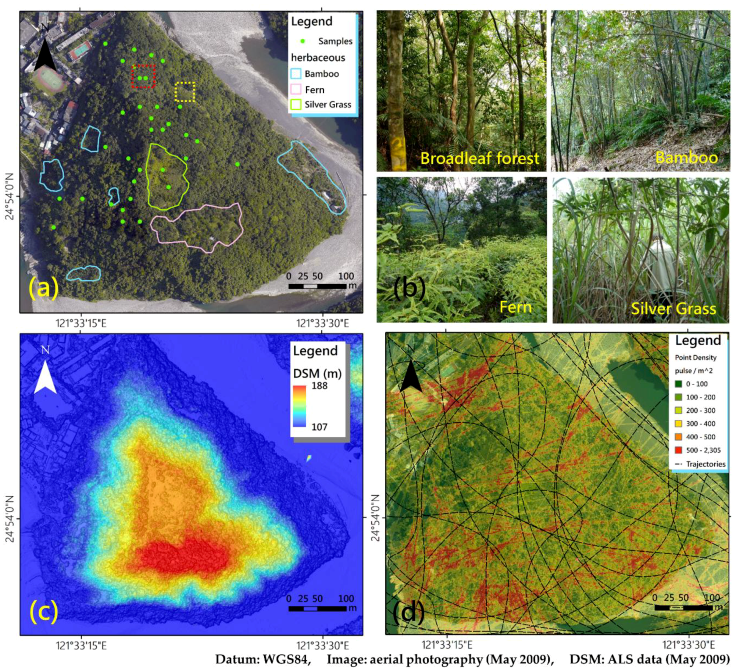
The study area was a tropical broadleaf forest located in the upstream section of the Nanshi River in Xindian District of New Taipei City, Taiwan. The dominant species in the study area include the Formosa acacia (Acacia confusa Merr.), camphor tree (Cinnamomum camphora (L.) J. Presl), common elaeocarpus (Elaeocarpus sylvestris (Lour.) Poir.), and turn in the wind (Mallotus paniculatus (Lam.) Muell.-Arg.). Their diameter at breast height ranged between 20 and 25 cm (based on in-situ measurement of 42 trees) and their height ranged between 10 and 15 m (based on 42 trees by using ALS data). Three types of herbaceous plants were widely distributed throughout the study area, namely, bamboo (Phyllostachys makinoi Hayata), fern (Dicranopteris dichotoma (Burm. f.) Underw.), and silver grass (Miscanthus floridulus (Labill.) Warb. ex K. Schum. & Lauterb.). The distribution of herbaceous plants in the study area is shown in Figure 1a based on aerial photographs with a 10 cm image resolution (taken simultaneously with LiDAR scanning) that were digitalized manually. In-situ plant photographs are shown in Figure 1b. The approximate area of the study area was 18.5 ha, and the study area was triangular in shape. Its height above sea level ranged between 107 and 188 m. The topographic map is presented in Figure 1c. As the research objective was to explore the stand density of wood plants, herbaceous plant areas were excluded.
2.2. ALS Dataset
This study used an Optech ALTM 3070 with a laser source wavelength of 1064 nm to collect point data. Scanning was conducted in May 2009. The instrument was carried by a helicopter. The flight altitude was 500 m (AGL), the PRF was 70 kHz, the scan frequency was 40 Hz, and the scan angle was ±18°. LiDAR data with a high density averaging 225.5 pulse/m2 was obtained using repetitive scanning of the study area in 20 flight lines. The point cloud density and flight trajectory are shown in Figure 1d. The Optech ALTM 3070 could record a maximum of four echo numbers. The las 1.2 LiDAR format [33] recorded the coordinates and intensity of each echo number.
2.3. In-Situ Measurements
The in-situ stand density was measured in 35 sample regions, each of which had an area of 10 m × 10 m (marked as green dots in Figure 1a). In-situ measurements were conducted on 18 October 2016, approximately seven years after LiDAR scanning. Nevertheless, the author continuously explored the study area between 2009 and 2016 and discovered that the area did not experience any large-scale interferences caused by events such as typhoons or developmental projects. No trees had fallen in the 35 sample regions. Furthermore, the area serves as a water conservation area for Feitsui Dam in which any development is prohibited. With regard to geographic coordinates, handheld GARMIN Dakota 20 GNSS was applied to calculate the average from 100 continuous measurements at the center point of each region. The instrument indicated that the horizontal error was smaller than 1 m. In accordance with the forest resource survey standards set by the Food and Agriculture Organization (FAO) [34], trees higher than 5 m were selected to measure stand density. The 35 regions contained 197 trees in total. The average stand density in the sample regions was 5.6 (trees/100 m2), with a standard deviation of 2.82 (trees/100 m2). The smallest and largest stand densities were 1 and 10, respectively. Sample regions were selected mainly based on their accessibility for personnel. Therefore, the sample regions were concentrated in the western and northern parts of the study area. The remaining part of the study area consisted of high and steep grounds that were impossible to access.
3. Methods
3.1. Steps of Stand Density Estimation
This study employed a raster-based method to calculate stand density. The stand density estimation procedure is shown in Figure 2. The first step was LiDAR processing, in which point clouds with similar echoes were used to generate a DSM, whereas point clouds of ground points were used to generate a DEM. Point clouds were converted into raster data using the triangulated irregular network (TIN) method. The TIN method is based on Delaunay triangles in three-dimensional space where the continuous surface is interpolated from the elevation values at the triangle nodes (the point clouds). The values of raster data were interpolated to the centers of the raster from this continuous surface [35]. Finally, a CHM was obtained by calculating the difference between the two models. The second step was the treetop extraction step. The local maximum method was used to determine the positions of treetops, which were then converted into stand density. A regression function between the stand density and in-situ stand density measurements was constructed. Further, the regression function was used to correct the stand density of the whole area to produce the final stand density map.
3.2. DSM, DEM and CHM Generation
In this study, three types of DSM were generated, namely, DSMFe, DSMLe, and DSMHFe. In the DSMFe, first-echo points were used to generate the DSM. In the DSMLe, last-echo points were used to generate the DSM. In the DSMHFe, first-echo points were selected and designated as the highest first-echo values within pixels.
In DEM generation, the first step involves the use of the Terrascan automatic classification software to classify point cloud data as ground points. Manual programming is then applied to the ground point classification results. Finally, a DEM is generated using the ground points. The TIN interpolation method is used in both DSM and DEM generation, with point clouds converted into raster data.
CHMFe was obtained based on the difference between DSMFe and DEM. Furthermore, the same procedure was applied for DSMLe and DSMHFe to obtain CHMLe and CHMHFe, respectively.
In order to investigate the effects of CHM cell size on the stand density estimation, the cell sizes of 1 m, 0.5 m, and 0.2 m were implemented for DSM and DEM generation.
3.3. Stand Density Estimaion From Treetop Extraction Using the Local Maximum Method
In stand density estimation, it was assumed that each tree has a treetop. Thus, the local maximum method could be used to determine treetop positions by applying a filter with a kernel size (). The number of treetops within an area unit was calculated and converted to stand density. Within a kernel, when the elevation of the central pixel is higher than its neighboring pixels, the central pixel is marked as a treetop [36,37]. To correctly estimate the treetop position, the local maximum method relies on testing different kernel sizes. Excessively large and small may affect the results. Therefore, for the Csizes of 1 m and 0.5 m, of 3 × 3, 5 × 5, and 7 × 7 were tested. For the Csize of 0.2 m, of 3 × 3, 5 × 5, 7 × 7, 9 × 9, 11 × 11, and 15 × 15 were tested. The main objective was to obtain the best results with the lowest error.
This study followed FAO standards [34] when determining the treetop positions and only considered trees that were higher than 5 m. Thus, the height threshold was set to 5 m. However, the CHMLe did not indicate tree height; therefore, the height threshold for the CHMLe was set to 2 m, which is the maximal height of grasslands and ferns. It should be noted that this study used three types of CHM data (CHMFe, CHMLe, and CHMHFe) in the local maximum method calculation and used two parameters, namely, Csize (1 m, 0.5 m, and 0.2 m) and (from 3 × 3 to 15 × 15).
3.4. Regression-Based Correction Method
To ease the burden of finding an appropriate set of and Csize parameters for suitable CHM data (i.e., CHMFe, CHMLe, or CHMHFe), this chapter investigates the use of regression models to adjust the stand density in LiDAR estimations. This method used three different regression models, i.e., linear, quadratic, and cubic, to build relations between independent () and dependent () variables using MATLAB software. It was found that the quadratic model had the best fit for the 35 pairs of the in-situ sample region () and the LiDAR estimated stand density (). Therefore, the quadratic model was employed to build relations, as shown in Formula (1).
During the regression model building process, the , , and values of the and regression equations were obtained. Thus, the post-correction value could be obtained by including the value in the regression equation. Due to the possibility of two value solutions in the quadratic regression model, this study selected the value that was showing an increasing trend in the regression model.
3.5. Error Assessment
This study explored stand density errors in LiDAR and in-situ estimations using three indicators, which were (root mean square error), commission error (), and omission error (). Data from 35 ( = 35) in-situ sample regions was obtained. The stand density estimated through in-situ measurements and the stand density estimated using LiDAR data in the th sample region were indicated as and , respectively.
The mainly explained stand density errors in LiDAR estimations. The value was calculated as shown in Formula (2).
The number of commission errors for stand density in the th sample region is shown in Formula (3),
The commission error ratio for the entire study area is shown in Formula (4),
where is shown in Formula (5),
The number of omission errors for stand density in the th sample region is shown in Formula (6),
The omission error ratio for the entire study area is shown in Formula (7),
3.6. Leave-One-Out Cross-Validation
The cross-validation (CV) method is often used in statistics to choose representative samples and build regression models. This study applied leave-one-out cross-validation (LOOCV) to test stand density errors in in-situ and LiDAR estimations as determined by the regression model. LOOCV was used because it only selects one sample as the test data, with the remaining samples included in the training data. The procedure is repeated until each sample has served as the test data. Using only one sample as the test data is beneficial for regression models with a relatively small sample size. Therefore, LOOCV was used in this study given the sample size of 35. With regard to LOOCV calculations, for samples, there are cross-validation errors. The error of the jth cross-validation sample is indicated as and is calculated as shown in Formula (8),
and is calculated as shown in Formula (9),
The error assessment had calculating commission error (), omission error (), and the formulas for which are shown below:
The number of commission errors for stand density in the th sample region is shown in Formula (10),
The commission error ratio for the entire study area is shown in Formula (11),
The number of omission errors for stand density in the th sample region is shown in Formula (12),
The omission error ratio for the entire study area is shown in Formula (13),
The is calculated as shown in Formula (14).
3.7. Numerical LiDAR Data Thinning
The average laser pulse density of the LiDAR data in this study was 225.5 pulse/m2, which is considered to be a high pulse density. Therefore, random sampling was used to thin the LiDAR data into different laser pulse densities. It should be noted that during random sampling, the laser pulses were different each time, which could cause differences between treetop positions and values. Thus, 30-fold random sampling was applied. Boxplots were drawn to demonstrate the influence of laser pulse density on and , where was the stand density estimated using the LiDAR data and corrected using regression models as described in Section 3.4. It is commonly believed that 30 is a large enough sample size. Therefore, this study obtained 30 samples using random sampling instead of using a single sample [38,39]. With regard to laser pulse density thinning, this study used DSM, DEM, and CHM data for the Csizes of 1 m, 0.5 m, and 0.2 m; for the generation of 1 m and 0.5 m DSM, DEM, and CHM data, LiDAR data was thinned to 1, 2, 3, 4, 5, 10, 20, 30, 40, and 50 pulse/m2. However, as the 0.2 m Csize required a higher laser pulse density to obtain the best DSM, DEM, and CHM data, the LiDAR data was thinned to 25, 50, 75, 100, 125, 150, 175, and 200 pulse/m2.
4. Results
The stand density of a tropical broadleaf forest was estimated from three types of CHM, namely, CHMFe, CHMLe, and CHMHFe, using the local maximum method, and the error assessment for each CHM with different cell sizes (1, 0.5, and 0.2 m) was conducted. The evaluation of the effectiveness of the regression-based correction method was performed. Finally, a comparison of estimated stand density at different laser pulse densities was conducted.
4.1. Comparison of Three Types CHM Data
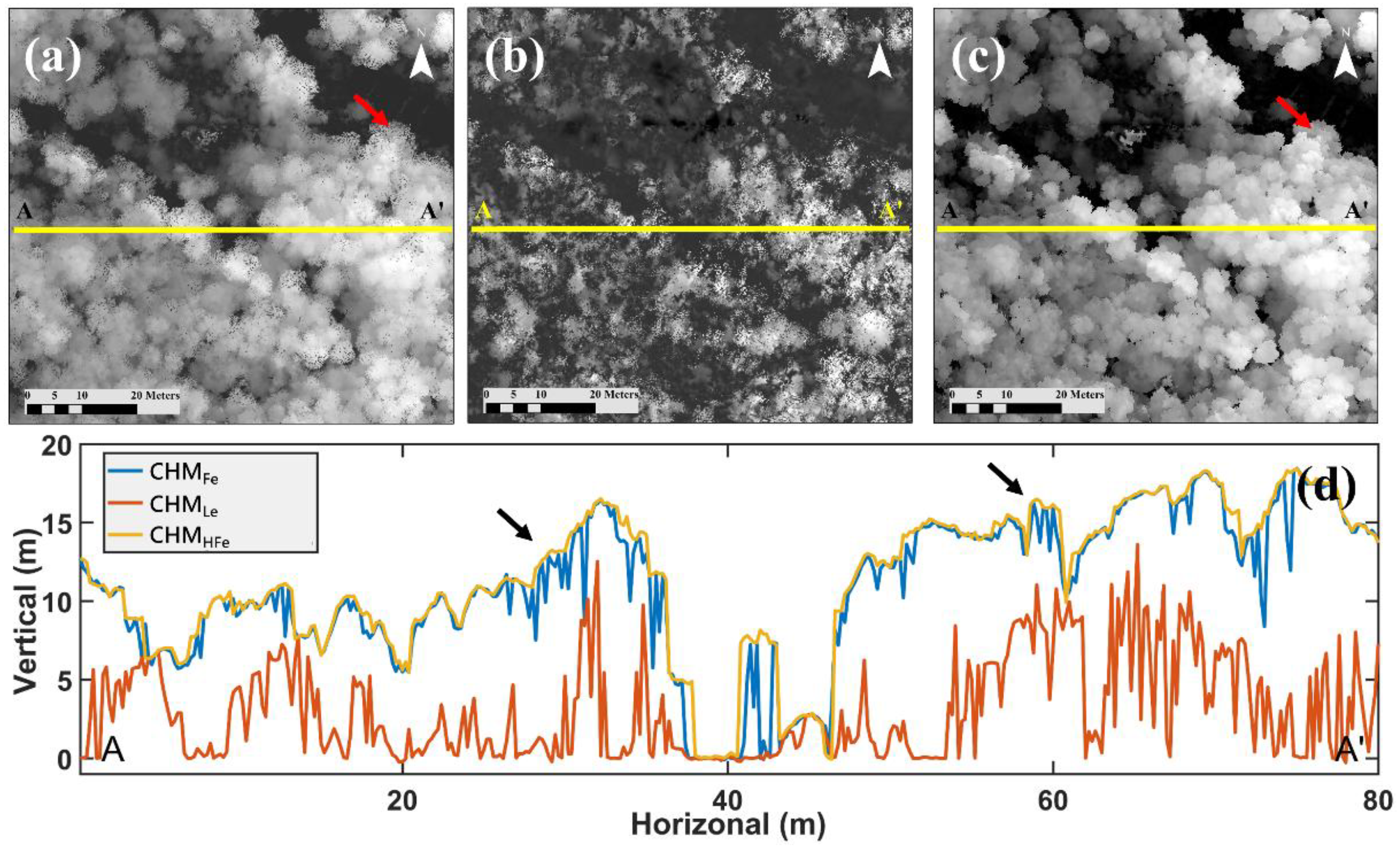
In this study, CHMFe, CHMLe, and CHMHFe data was generated. A small area was selected to explain features of the three types of CHM data (yellow dotted line in Figure 1a), as shown in Figure 3a–c, where the CHM has the Csize of 0.2 m. The results showed that in CHMFe, the tree crown edges (marked by the red arrow in Figure 3a) had formed pepper-like pits. The tree crown edges of CHMHFe were much more distinctive than those in CHMFe and had much fewer pits (marked by the red arrow in Figure 3c). However, the tree crowns were not visible in CHMLe because it was produced using last-echoes (Figure 3b). Figure 3d shows the cross-section of the three types of CHM data along profiles A–A’ (denoted as a straight yellow line in Figure 3a–c) with the cross-section width of 0.2 m. Clear differences can be observed in the three cross-sections. CHMHFe and CHMFe are almost the same and they are consistently higher than CHMLe. On some occasions, pits can be found in CHMFe, where CHMFe is lower than CHMHFe (denoted as black arrows in Figure 3d).
4.2. Stand Density by the Local Maximum Method
With regard to stand density estimated using LiDAR data, three types of data were obtained, namely, CHMFe, CHMLe, and CHMHFe data. The local maximum method was used to estimate stand density. All related parameters are described in Section 3.3. Three indicators were used in the assessment of stand density errors in LiDAR estimations, namely , , and . The results are presented in Table 1.
The results showed that (Table 1) directly affected the stand density value. When Csize remained unchanged, decreased substantially with increasing . For example, when Csize = 1 m, was 232 (trees/100 m2) and 31 (trees/100 m2) when was 3 and 7, respectively. The results for other Csizes were similar.
With regard to and , it was desirable to find a set of appropriate and Csize with matching CHM data that had both small and , which means low commission and omission errors for estimating tree density. It was found that (Table 1) extremely low values were usually associated with large values, and vice versa. When limiting both the and to an arbitrary threshold value of 0.15, only four cases were found. They are CHMFe with Csize = 0.5 m and = 5 ( = 0.07, = 0.14), CHMFe with Csize = 0.2 m and = 11 ( = 0.08, = 0.14), CHMLe with Csize = 0.2 m and = 15 ( = 0.11, = 0.13), and CHMHFe with Csize = 0.5 m and = 5 ( = 0.10, = 0.15). Among the four cases, the values were between 0.14 and 0.15, while the as small as 0.07 could be achieved. Thus, CHMFe data with Csize = 0.5 m and = 5 indicate the best combination for the local maximum method in our study area.
The minimum for CHMFe, CHMLe, and CHMHFe, obtained at Csize = 1 m, was 2.00, 2.56, and 2.58 trees/100 m2 (each denoted as a black star in Table 1), respectively; and the corresponding for all was 3. The minimum obtained at Csize = 0.5 m was 1.68, 2.43, and 2.19 trees/100 m2 (each denoted as black star in Table 1), respectively; and the respective values were 5, 7, and 5. The minimum obtained at Csize = 0.2 m was 1.73, 1.94, and 2.43 trees/100 m2 (each denoted as a black star in Table 1), respectively; the respective values were 11, 15, and 13. Thus, the minimum found in the three types of CHM ranged between 1.68 and 2.43 trees/100 m2. Furthermore, the difference of only 0.78 (trees/100 m2) indicated that all three types of CHM data, CHMFe, CHMLe, and CHMHFe, could be used to estimate stand density. Similarly, the three kinds of Csizes, 1 m, 0.5 m, and 0.2 m, could all be used to estimate stand density. Finally, the minimum of 1.68 and average = 5.2 were observed when the CHMFe parameters were Csize = 0.5 m and = 5. Thus, the best stand density estimate was 5.2 ± 1.68 (trees/100 m2) for our study area.
4.3. Using Leave-One-Out Cross-Validation to Test Stand Density Errors
There are 35 samples in this study. Thirty-four samples were chosen for the LOOCV (training sample) to build a regression model and one sample (test data) was selected to estimate the error value. Therefore, there were 35 values and one value for each parameter, as shown in Table 2. For the error of stand density when using the LOOCV method, the minimum was between 0.01 and 0.45, the maximum was between 3.52 and 14.93, the average was between 1.24 and 4.12, and the was between 1.79 and 4.94. The values were compared with the values in Table 1; the minimum (1.79) was the same as the minimum (1.68). Besides, the maximum and were reduced from 108.5 to 4.94, which means that the regression-based correction method is effective for reducing the error.
4.4. Stand Density Map by the Regression-Based Correction Method
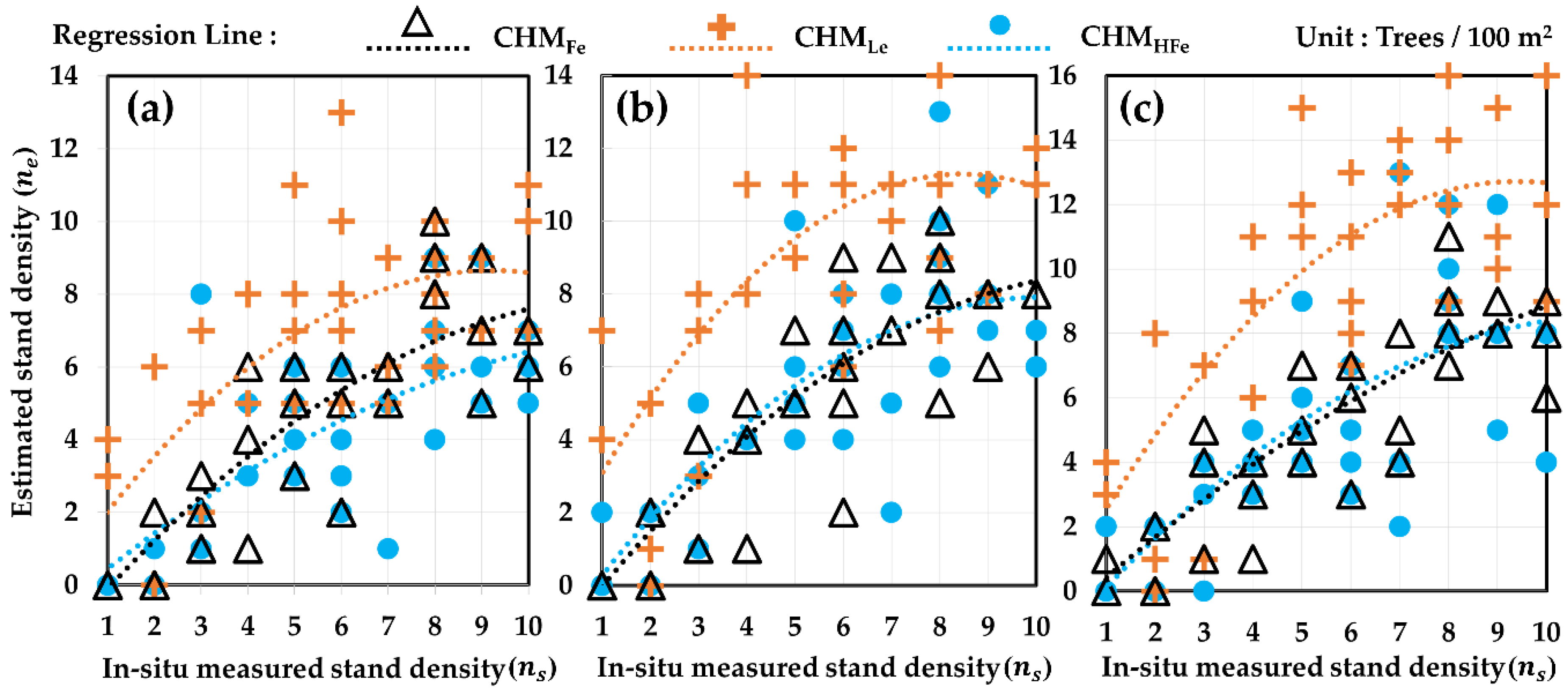
In Figure 4a–c, the Csizes are 1 m, 0.5 m, and 0.2 m and the values are 3, 5, and 11. These Csize and parameters were selected based on the CHMFe that had the minimum . The quadratic regression models for CHMFe, CHMLe, and CHMHFe are presented. The maximum value of stand density in in-situ measurements was 10. Furthermore, in-situ stand densities measurement composed the X axis (independent variable) and LiDAR-estimated stand density composed the Y axis (dependent variable). Figure 4a–c show that both LiDAR-estimated and in-situ stand densities have an increasing trend in the quadratic regression models, indicating that LiDAR data can be used to effectively estimate the stand density of tropical forests.
This study used all 35 in-situ measurement samples (which were stand densities) to calculate , , and values in the quadratic regression models, which were used to calculate and , as well as to calculate the , , and of error assessment values, as shown in Table 3. With regard to values, they were largely similar under each estimation parameter. Therefore, they are omitted in Table 3 and are only discussed below. The values ranged between 241.63 and 195.72, with an average of = 208.32. The average and ( = 197) difference was only 11.32, indicating that the difference between the LiDAR estimated and in-situ-measured stand densities corrected using the regression models was approximately 6%. Table 3 shows the , , and values. The maximum and minimum values were 0.35 and 0.12, respectively; the average was 0.2 and its standard deviation was 0.04. The maximum and minimum values were 0.21 and 0.10, respectively; the average was 0.14 and its standard deviation was 0.02. With regard to , its maximum value was 4.88, its minimum value was 1.74, its average value was 2.66, and its standard deviation was 0.58. Furthermore, a comparison of the and showed that the maximum value decreased from 108.5 to 4.88, the minimum value slightly increased from 1.68 to 1.74, the average value decreased from 12.35 to 2.66, and the standard deviation decreased from 21.95 to 0.58. Thus, these results indicated that regression models could effectively correct stand density errors. It is worth noting that when a minimum value was obtained (star marks in Table 1), it is not necessary to correct the stand density estimation using the regression model. For example, in Table 1 and Table 3, the value in CHMFe (Csize = 0.5 m; = 5) is 1.68 and the value is slightly increased to 2.17, indicating that when is at its minimum, the stand density estimation should not be corrected using regression models. As shown in Table 3, when CHMFe parameters were Csize = 0.5 m and = 7, an value of 1.74 was the minimum value, and the average = 5.95; thus, the best result after stand density correction using regression models was 5.95 ± 1.74 (trees/100 m2).
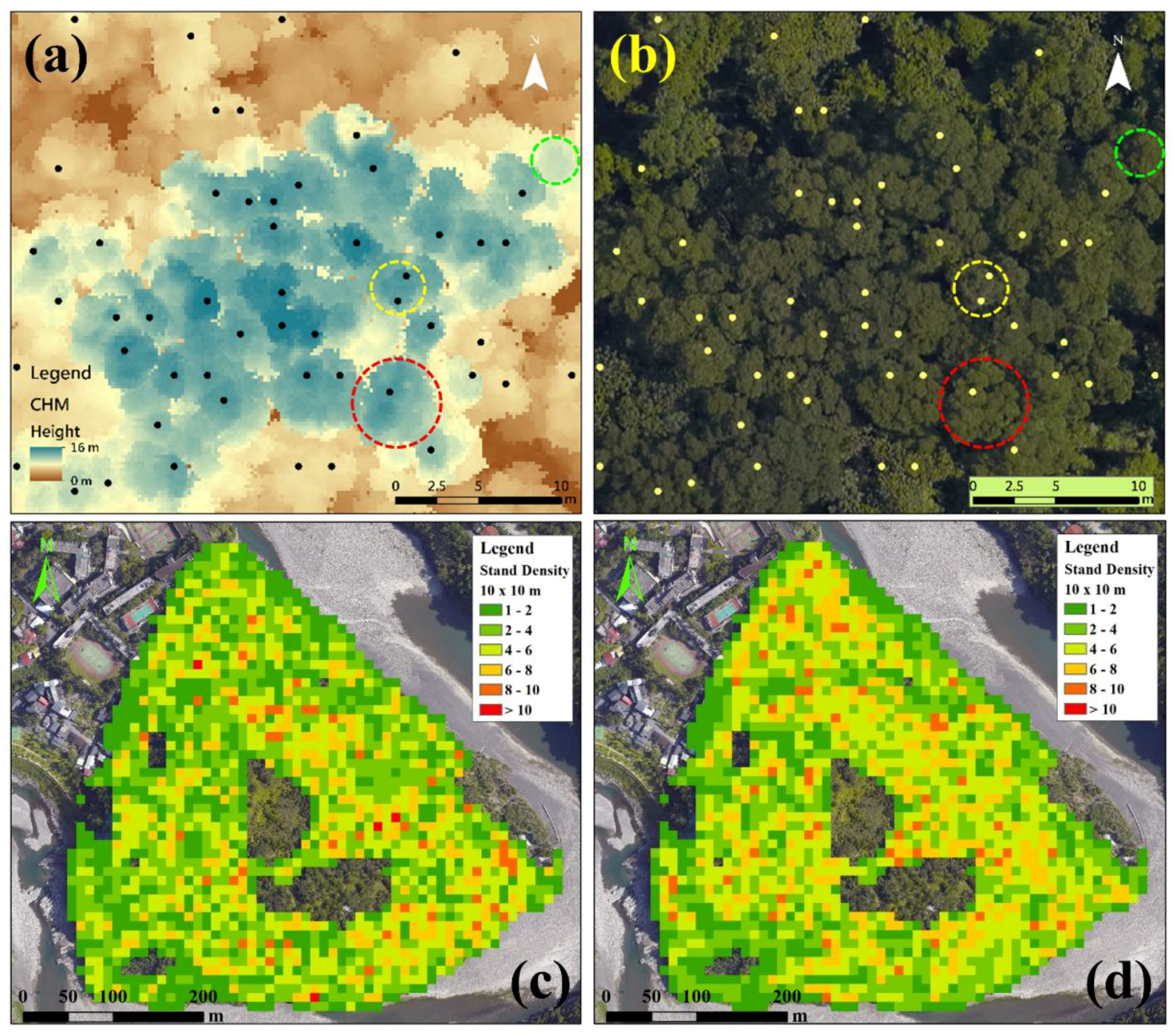
For the purpose of giving the best visual demonstration, the treetop positions extracted from CHMHFe (with Csize = 0.2 m and = 11; having = 1.73) using the local maximum method were marked by black dots overlaid on CHMHFe (Figure 5a) and by yellow dots overlaid on the orthophoto of a 10 cm ground resolution (Figure 5b). It was found that many treetops were nicely located inside the tree crown (an example denoted by the red dotted line in Figure 5a,b). There are also a few cases where two (an example denoted by the yellow dotted line in Figure 5a,b) or none (an example denoted by the green dotted line) of the tree tops are found inside a tree crown.
The minimum (1.68) was obtained from CHMFe with Csize = 0.5 m and = 5; these parameters were used to draw the stand density map as shown in Figure 5c, where the regions of herbaceous plants (in Figure 1a) were excluded. A total of 6575 trees (higher than 5 m) was computed by summing all the 10 m × 10 m cells of the tree density map. Furthermore, the average stand density was 4.34 trees/100 m2.
In order to demonstrate the advantage of the proposed regression-based correction for estimating tree density, we selected the results with the maximum (108.5) in Table 1 where CHMLe was used with Csize = 0.2 m and = 3. After correction, the value was reduced to 2.76. Furthermore, the corrected stand density map is shown in Figure 5d, where a total of 6637 trees (higher than 5 m) was estimated, with an average tree density of 4.01 trees/100 m2. It is noted that the tree density map produced directly by the maximum local method, with the smallest (Figure 5c), is very similar to that produced by the regression-based correction method (which had a very large value before correction; Figure 5d). To further demonstrate their difference, the histogram (Figure 6) of the difference of these two maps was produced by subtracting the uncorrected result (Figure 5c) from the regression-corrected result (Figure 5d) at corresponding 10 m × 10 m cells. It was found that almost half (49%) of the 10 m × 10 m cells were within the range between −1.5 and 1.5 trees/100 m2, and a great portion (19%) of the cells were within the range between −0.5 and 0.5, indicating that two stand density maps had a high degree of similarity.
4.5. Error Assessment of Stand Density Estimation at Different Laser Pulse Densities
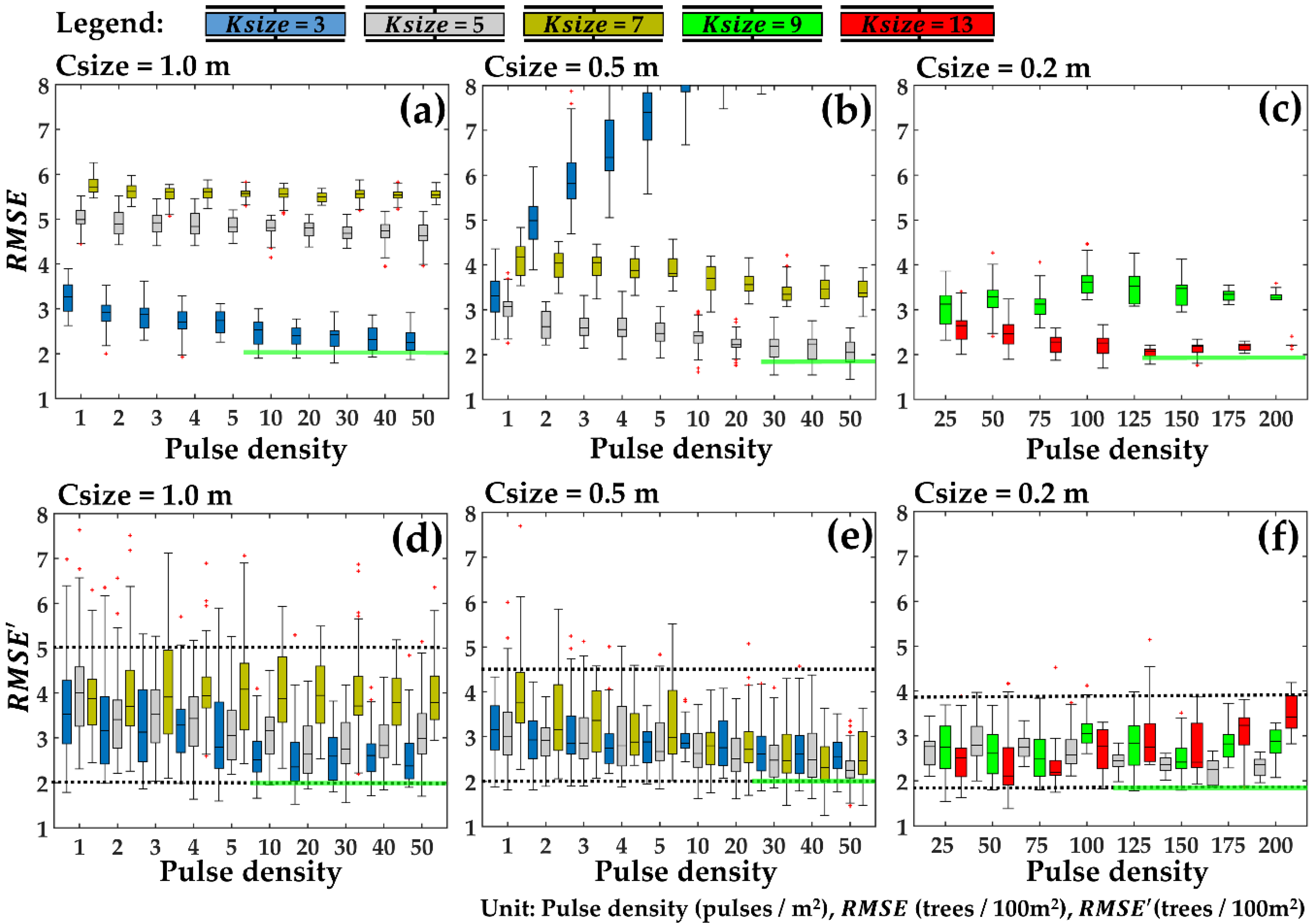
Figure 7a–c show changes in values at different laser pulse densities in CHMFe. Figure 7d–f show changes in values at different laser pulse densities in CHMFe. Boxplots were obtained through 30-fold sampling, as described in Section 3.7. In Figure 7a,d, Figure 7b,e, and Figure 7c,f, Csizes were 1 m, 0.5 m, and 0.2 m, respectively. As the CHMFe results largely corresponded to those of CHMLe and CHMHFe, CHMFe was selected as the example.
As shown in Figure 7a, when = 3, decreased as laser pulse density increased. When the laser pulse density reached 10 pulses/m2, however, the could no longer decrease. The final trend results formed a smooth line (indicated by a green line in the figure) and indicated that at Csize = 1 m, a laser pulse density of 10 pulses/m2 was sufficient. Thus, the results in Figure 7a–c indicated that at Csizes of 1 m, 0.5 m, and 0.2 m, sufficient laser pulse densities were 10, 30, and 125 pulses/m2, respectively. In Figure 7d, values ranged between 5 and 2 (black dotted line). At = 3, decreased with an increase in laser pulse density. No reduction trend was observed after the laser pulse density reached 10 pulses/m2, which corresponded to the results. The results indicated that laser pulse density influenced and values; however, excessively high laser pulse densities were not helpful.
5. Discussions
Remote sensing is an effective tool to estimate the stand density. Results from relevant literature are shown in Table 4, where the remote sensing data used included airborne [40] and terrestrial LiDAR [41], optical imagery [42,43,44], and SAR data [45]. The study reported by Lee and Lucas [40] is most directly comparable to ours as they also implemented airborne LiDAR data (Optech ALTM 1020), while the stand densities were estimated by computing the height-scaled crown openness index for LiDAR data of white cypress pine in the coniferous forest. Among their results, the minimum value was 1.33 trees/100 m2. Palace, et al. [41] reported the use of terrestrial LiDAR to estimate the stand density of a closed canopy in a tropical forest, where individual treetops were detected based on the relative vegetation profiles and fast Fourier transform technique. Among their results, the minimum value of 1.53 trees/100 m2.
Three reported studies were founded using optical imagery to estimate stand density. Kahriman, et al. [42] used Landsat TM satellite imagery to estimate the stand density based on establishing multiple regression between vegetation indices, including the soil adjusted vegetation index and difference vegetation index, and stand density for a mixed forest of Pine and beech. Furthermore, their reported minimum value was 0.83 trees/100 m2. Chrysafis, et al. [43] used Landsat 8 OLI satellite imagery to estimate the stand density based on the random forest regression algorithm by establishing the relationship between spectral information and stand density for a coniferous forest (black pine and oaks). Among their results, the minimum value was 2.57 trees/100 m2. Mohammadi, et al. [44] used Landsat ETM+ satellite imagery to estimate stand density based on the multivariate regression model established between band 4 and 5 of ETM+ imagery and in-situ stand density in a mixed hornbeam and oak forest. Among their results, the minimum value was 1.70 trees/100 m2.
The stand density estimation from JERS-1 SAR satellite imagery reported by Wang and Qi [45] was conducted based on a radiative transfer inversion model for mixed deciduous and dry evergreen forests. Their value was 1.61 trees/100 m2.
Overall, the of stand densities obtained from the above mentioned studies were between 0.83 and 2.57 trees/100m2. Our results had the minimum of 1.68, which was comparable with these reported values and indicated that our results could effectively estimate the stand density in a tropical forest. Furthermore, the average value by the proposed regression based correction method was 2.66 (Table 3), which was similar to these reported values (0.83–2.57) and indicated that regression models could effectively correct stand density errors.
In this study, we included CHMHFe because it was reported that a pit-free CHM [26] was essential for accurate short tree detection. In turn, it was logical to postulate that an accurate stand tree density estimate can be achieved by CHMHFe. However, an unexpected result showed that CHMFe was more suitable to estimate stand density, and when having the same Csize, the minimum of CHMFe was consistently smaller than that of CHMHFe (Table 1). For example, when Csize = 1 m, the minimum of CHMFe and CHMHFe was 2.00 vs. 2.58; when Csize = 0.5 m, the minimum of CHMFe and CHMHFe was 1.68 vs. 2.19; when Csize = 0.2 m, the minimum of CHMFe and CHMHFe was 1.73 vs. 2.43. This indicated that CHMFe was more suitable for our study area.
6. Conclusions
This study used first-echo, last-echo, and highest first-echo ALS data to generate three types of CHM data, i.e., CHMFe, CHMLe, and CHMHFe, respectively; Csizes of 1 m, 0.5 m, and 0.2 m were applied to each data type. The local maximum method was used to detect treetops that were then converted into stand density. In-situ measurements were performed for stand density in 35 sample regions (10 × 10 m). After an exhaustive search of different values (Table 1), the results indicated that the ranged between 1.68 and 2.43 across three CHMs and three Csizes. This concludes that the stand density can be reasonably estimated by LiDAR data using the local maximum method with appropriate sets of and Csize parameters. The difference was only 0.78, indicating that stand density was effectively estimated in both cases, using the three CHM and the three Csizes. The minimum of 1.68 and average = 5.2 were observed when the CHMFe parameters were Csize = 0.5 m and = 5. Thus, the best estimate for the stand density result for our sample regions was 5.2 ± 1.68 (trees/100 m2).
The CHM data, Csize, and that produced the minimum error results ( = 1.68) were used to draw a stand density map for the study area. The map contained 1516 (10 × 10 m) pixels. In total, 6575 trees were higher than 5 m, and the average stand density was 4.34 (trees/100 m2).
To ease the burden of finding an appropriate set of and Csize parameters for suitable CHM data, this study proposed a regression-based stand density estimation method. In-situ stand density measurements were set as an independent variable and stand density, estimated using LiDAR data, was set as a dependent variable.
Furthermore, regression models were used to correct the error in stand density estimations; the after correction was designated as . A comparison of the and showed that the maximum value decreased from 108.5 to 4.88, the minimum value slightly increased from 1.68 to 1.74, the average value decreased from 12.35 to 2.66, and the standard deviation decreased from 21.95 to 0.58. Thus, the results indicated that regression models could effectively correct stand density errors. When the CHMFe parameters were Csize = 0.5 m and = 7, of 1.74 was the minimum value, and the average = 5.95; thus, the best result with the minimum after stand density correction was 5.95 ± 1.74 (trees/100 m2). It is worth noting that when a minimum value was obtained (star marks in Table 1), it was not necessary to correct the stand density estimation using the regression model. For example, in Table 3, the value in CHMFe (Csize = 0.5 m; = 5) is 1.68 and the value increases by 0.49 to 2.17, indicating that when is the minimum value, the error should not be corrected using regression models.
Finally, with regard to evaluating the stand density estimation of different laser pulse densities, it was shown that values decreased with an increase in laser pulse density. No reduction trend was observed in values when the laser pulse density reached 10 (Csize = 1 m), 30 (Csize = 0.5 m), and 125 (Csize = 0.2 m) pulses/m2. The results indicated that laser pulse density influenced and values; however, excessively high laser pulse densities were not helpful. In other words, at a Csize of 1 m, the laser pulse density must exceed 10 pulses/m2 to reduce the stand density error.
Author Contributions
C.C.L. performed this study, developed the methodology, analyzed the data, and wrote the manuscript. C.K.W. designed this study, contributed to the design of the study, and provided technical oversight of the project. All authors discussed and edited the paper.
Funding
This research was funded by Department of Land Administration, Ministry of Interior, Taiwan grant number 106SU1215. We were also supported by the Dr. Winston H. Chen scholarship of the NCKU Research and Development Foundation. The APC was funded by Department of Land Administration, Ministry of Interior, Taiwan.
Acknowledgments
We appreciate the anonymous reviewers and the editor for thoughtful feedback that improved the manuscript.
Conflicts of Interest
The authors declare no conflict of interest.
References
- Lorimer, C.G.; White, A.S. Scale and frequency of natural disturbances in the northeastern US: Implications for early successional forest habitats and regional age distributions. For. Ecol. Manag. 2003, 185, 41–64. [Google Scholar] [CrossRef]
- Espirito-Santo, F.D.B.; Gloor, M.; Keller, M.; Malhi, Y.; Saatchi, S.; Nelson, B.; Oliveira, R.C.; Pereira, C.; Lloyd, J.; Frolking, S.; et al. Size and frequency of natural forest disturbances and the Amazon forest carbon balance. Nat. Commun. 2014, 5, 3434. [Google Scholar] [CrossRef] [PubMed] [Green Version]
- Zeide, B. How to measure stand density. TreesStruct. Funct. 2005, 19, 1–14. [Google Scholar] [CrossRef]
- Keddy, P.A. Plants and Vegetation: Origins, Processes, Consequences; Cambridge University Press: Cambridge, UK; New York, NY, USA, 2007; p. 683. [Google Scholar]
- Ulvcrona, K.A.; Claesson, S.; Sahlen, K.; Lundmark, T. The effects of timing of pre-commercial thinning and stand density on stem form and branch characteristics of Pinus sylvestris. Forestry 2007, 80, 323–335. [Google Scholar] [CrossRef]
- Franklin, O.; Aoki, K.; Seidl, R. A generic model of thinning and stand density effects on forest growth, mortality and net increment. Ann. For. Sci. 2009, 66, 815. [Google Scholar] [CrossRef]
- Wu, Y.C.; Strahler, A.H. Remote estimation of crown size, stand density, and biomass on the Oregon transect. Ecol. Appl. 1994, 4, 299–312. [Google Scholar] [CrossRef]
- Sousa, V.B.; Louzada, J.L.; Pereira, H. Variation of ring width and wood density in two unmanaged stands of the Mediterranean Oak Quercus faginea. Forests 2018, 9, 44. [Google Scholar] [CrossRef]
- Cheng, X.R.; Yu, M.K.; Wu, T.G. Effect of forest structural change on carbon storage in a coastal metasequoia glyptostroboides stand. Sci. World J. 2013, 2013, 830509. [Google Scholar] [CrossRef] [PubMed]
- Uhl, E.; Biber, P.; Ulbricht, M.; Heym, M.; Horváth, T.; Lakatos, F.; Gál, J.; Steinacker, L.; Tonon, G.; Ventura, M.; et al. Analysing the effect of stand density and site conditions on structure and growth of oak species using Nelder trials along an environmental gradient: Experimental design, evaluation methods, and results. For. Ecosyst. 2015, 2, 17. [Google Scholar] [CrossRef]
- Moon, M.; Kim, T.; Park, J.; Cho, S.; Ryu, D.; Kim, H.S. Variation in sap flux density and its effect on stand transpiration estimates of Korean pine stands. J. For. Res. 2015, 20, 85–93. [Google Scholar] [CrossRef]
- Humagain, K.; Portillo-Quintero, C.; Cox, R.D.; Cain, J.W. Mapping tree density in forests of the southwestern USA using Landsat 8 data. Forests 2017, 8, 287. [Google Scholar] [CrossRef]
- Wulder, M.A.; White, J.C.; Nelson, R.F.; Naesset, E.; Orka, H.O.; Coops, N.C.; Hilker, T.; Bater, C.W.; Gobakken, T. LiDAR sampling for large-area forest characterization: A review. Remote Sens. Environ. 2012, 121, 196–209. [Google Scholar] [CrossRef]
- Popescu, S.C.; Wynne, R.H.; Nelson, R.F. Estimating plot-level tree heights with LiDAR: Local filtering with a canopy-height based variable window size. Comput. Electron. Agric. 2002, 37, 71–95. [Google Scholar] [CrossRef]
- Kwak, D.A.; Lee, W.K.; Lee, J.H.; Biging, G.S.; Gong, P. Detection of individual trees and estimation of tree height using LiDAR data. J. For. Res. 2007, 12, 425–434. [Google Scholar] [CrossRef]
- Barnes, C.; Balzter, H.; Barrett, K.; Eddy, J.; Milner, S.; Suarez, J.C. Individual tree crown delineation from airborne laser scanning for diseased larch forest stands. Remote Sens. 2017, 9, 231. [Google Scholar] [CrossRef]
- Gougeon, F.A. A crown-following approach to the automatic delineation of individual tree crowns in high spatial resolution aerial images. Can. J. Remote Sens. 1995, 21, 274–284. [Google Scholar] [CrossRef]
- Lin, C.S.; Thomson, G.; Popescu, S.C. An IPCC-compliant technique for forest carbon stock assessment using airborne LiDAR-derived tree metrics and competition Index. Remote Sens. 2016, 8, 528. [Google Scholar] [CrossRef]
- Koch, B.; Heyder, U.; Weinacker, H. Detection of individual tree crowns in airborne LiDAR data. Photogramm. Eng. Remote Sens. 2006, 72, 357–363. [Google Scholar] [CrossRef]
- Reitberger, J.; Schnorr, C.; Krzystek, P.; Stilla, U. 3D segmentation of single trees exploiting full waveform LiDAR data. ISPRS J. Photogramm. 2009, 64, 561–574. [Google Scholar] [CrossRef]
- Morsdorf, F.; Meier, E.; Allgöwer, B.; Nüesch, D. Clustering in airborne laser scanning raw data for segmentation of single trees. Int. Arch. Photogramm. Remote Sens. Spat. Inf. Sci. 2003, 34, 27–33. [Google Scholar]
- Vega, C.; Hamrouni, A.; El Mokhtari, S.; Morel, J.; Bock, J.; Renaud, J.P.; Bouvier, M.; Durrieu, S. PTrees: A point-based approach to forest tree extraction from LiDAR data. Int. J. Appl. Earth Obs. Geoinf. 2014, 33, 98–108. [Google Scholar] [CrossRef]
- Hu, X.; Chen, W.; Xu, W. Adaptive mean shift-based Identification of individual trees using airborne LiDAR Data. Remote Sens. 2017, 9, 148. [Google Scholar] [CrossRef]
- Van Leeuwen, M.; Coops, N.C.; Wulder, M.A. Canopy surface reconstruction from a LiDAR point cloud using Hough transform. Remote Sens. Lett. 2010, 1, 125–132. [Google Scholar] [CrossRef] [Green Version]
- Hyyppä, J.; Yu, X.W.; Hyyppä, H.; Vastaranta, M.; Holopainen, M.; Kukko, A.; Kaartinen, H.; Jaakkola, A.; Vaaja, M.; Koskinen, J.; et al. Advances in forest inventory using airborne laser scanning. Remote Sens. 2012, 4, 1190–1207. [Google Scholar] [CrossRef]
- Khosravipour, A.; Skidmore, A.K.; Isenburg, M.; Wang, T.J.; Hussin, Y.A. Generating pit-free canopy height models from airborne LiDAR. Photogramm. Eng. Remote Sens. 2014, 80, 863–872. [Google Scholar] [CrossRef]
- Soininen, A. TerraScan User’s Guide; Terrasolid Press: Helsinki, Finland, 2000; p. 592. [Google Scholar]
- Lee, C.C.; Wang, C.K. Effect of flying altitude and pulse repetition frequency on laser scanner penetration rate for digital elevation model generation in a tropical forest. GISci. Remote Sens. 2018, 1–22. [Google Scholar] [CrossRef]
- Popescu, S.C.; Wynne, R.H. Seeing the trees in the forest: Using LiDAR and multispectral data fusion with local filtering and variable window size for estimating tree height. Photogramm. Eng. Remote Sens. 2004, 70, 589–604. [Google Scholar] [CrossRef]
- Wang, Q.; Adiku, S.; Tenhunen, J.; Granier, A. On the relationship of NDVI with leaf area index in a deciduous forest site. Remote Sens. Environ. 2005, 94, 244–255. [Google Scholar] [CrossRef]
- Le Maire, G.; Marsden, C.; Nouvellon, Y.; Grinand, C.; Hakamada, R.; Stape, J.L.; Laclau, J.P. MODIS NDVI time-series allow the monitoring of Eucalyptus plantation biomass. Remote Sens. Environ. 2011, 115, 2613–2625. [Google Scholar] [CrossRef]
- Fernandez-Diaz, J.C.; Carter, W.E.; Glennie, C.; Shrestha, R.L.; Pan, Z.; Ekhtari, N.; Singhania, A.; Hauser, D.; Sartori, M. Capability assessment and performance metrics for the Titan multispectral mapping LiDAR. Remote Sens. 2016, 8, 939. [Google Scholar] [CrossRef]
- ASPRS. LAS Specification Version 1.4; American Society for Photogrammetry and Remote Sensing Press: Bethesda, MD, USA, 2011; p. 28. [Google Scholar]
- Keenan, R.J.; Reams, G.A.; Achard, F.; de Freitas, J.V.; Grainger, A.; Lindquist, E. Dynamics of global forest area: Results from the FAO global forest resources assessment 2015. For. Ecol. Manag. 2015, 352, 9–20. [Google Scholar] [CrossRef]
- Montealegre, A.L.; Lamelas, M.T.; de la Riva, J. Interpolation routines assessment in ALS-derived digital elevation models for forestry applications. Remote Sens. 2015, 7, 8631–8654. [Google Scholar] [CrossRef]
- Wulder, M.; Niemann, K.O.; Goodenough, D.G. Local maximum filtering for the extraction of tree locations and basal area from high spatial resolution imagery. Remote Sens. Environ. 2000, 73, 103–114. [Google Scholar] [CrossRef]
- Nelson, T.; Boots, B.; Wulder, M.A. Techniques for accuracy assessment of tree locations extracted from remotely sensed imagery. J. Environ. Manag. 2005, 74, 265–271. [Google Scholar] [CrossRef] [PubMed]
- Cohen, J. Things I have learned (so far). Am. Psychol. 1990, 45, 1304. [Google Scholar] [CrossRef]
- Kar, S.S.; Ramalingam, A. Is 30 the magic number? Issues in sample size estimation. Natl. J. Commun. Med. 2013, 4, 175–179. [Google Scholar]
- Lee, A.C.; Lucas, R.M. A LiDAR-derived canopy density model for tree stem and crown mapping in Australian forests. Remote Sens. Environ. 2007, 111, 493–518. [Google Scholar] [CrossRef]
- Palace, M.; Sullivan, F.B.; Ducey, M.; Herrick, C. Estimating tropical forest structure using a terrestrial LiDAR. PLoS ONE 2016, 11, e0154115. [Google Scholar] [CrossRef] [PubMed]
- Kahriman, A.; Gunlu, A.; Karahalil, U. Estimation of crown closure and tree density using Landsat TM satellite images in mixed forest stands. J. Indian Soc. Remote Sens. 2014, 42, 559–567. [Google Scholar] [CrossRef]
- Chrysafis, I.; Mallinis, G.; Gitas, I.; Tsakiri-Strati, M. Estimating Mediterranean forest parameters using multi seasonal Landsat 8 OLI imagery and an ensemble learning method. Remote Sens. Environ. 2017, 199, 154–166. [Google Scholar] [CrossRef]
- Mohammadi, J.; Joibary, S.S.; Yaghmaee, F.; Mahiny, A.S. Modelling forest stand volume and tree density using Landsat ETM plus data. Int. J. Remote Sens. 2010, 31, 2959–2975. [Google Scholar] [CrossRef]
- Wang, C.; Qi, J. Biophysical estimation in tropical forests using JERS-1 SAR and VNIR imagery. II. aboveground woody biomass. Int. J. Remote Sens. 2008, 29, 6827–6849. [Google Scholar] [CrossRef]
Figure 1.
Tropical broadleaf forest study area in Xindian District, New Taipei City, Taiwan. (a) Aerial photographs. The vegetation distribution in the figure includes tropical broadleaf forests, bamboo forests, ferns, and silver grass. The green dots indicate 35 sample regions examined using in-situ measurements. (b) In-situ photographs, including broadleaf forests, bamboo forests, ferns, and silver grass; (c) DSM figure (LiDAR generation) with additional shadow effects; (d) Laser pulse density and flight scanning trajectory.

Figure 2.
Stand density estimation procedure.
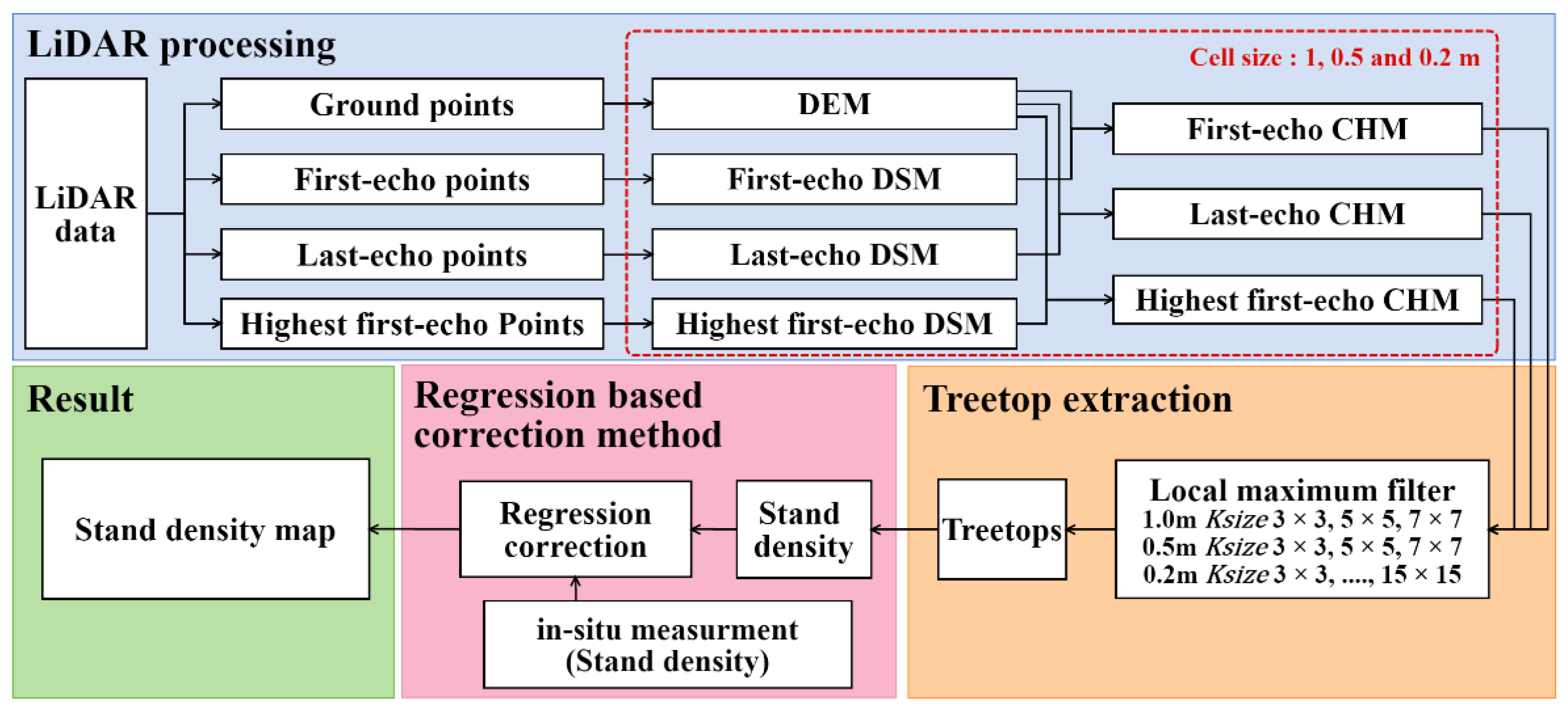
Figure 3.
Comparing features of three types of CHM data (Csize = 0.2 m). The range of (a–c) is marked in Figure 1a with a yellow dotted line. (a) CHMFe; (b) CHMLe; (c) CHMHFe; (d) Sectional views of three types of CHM data, marked by a yellow line from A to A’ in (a–c).
Figure 3.
Comparing features of three types of CHM data (Csize = 0.2 m). The range of (a–c) is marked in Figure 1a with a yellow dotted line. (a) CHMFe; (b) CHMLe; (c) CHMHFe; (d) Sectional views of three types of CHM data, marked by a yellow line from A to A’ in (a–c).

Figure 4.
Quadratic regression models built using in-situ stand density measurements and LiDAR-estimated stand density from the local maximum method. (a) Csize = 1 m and = 3; (b) Csize = 0.5 m and = 5; (c) Csize = 0.2 m and = 11.
Figure 4.
Quadratic regression models built using in-situ stand density measurements and LiDAR-estimated stand density from the local maximum method. (a) Csize = 1 m and = 3; (b) Csize = 0.5 m and = 5; (c) Csize = 0.2 m and = 11.

Figure 5.
The CHMHFe, treetop positions, and stand density map using LiDAR data. (a) the CHMHFe (Csize = 0.2 m) and treetop positions (using the local maximum method and marked by the black dots); (b) Aerial photographs and treetop positions (same as a and marked by the yellow dots). The range of (a,b) is marked in Figure 1a with a red dotted line; (c) Stand density map, which was using CHMFe and parameters that were Csize = 0.5 m and = 5; (d) Stand density map of regression corrected, which was using CHMLe and parameters that were Csize = 0.2 m and = 3.

Figure 6.
Frequency distribution histogram of the difference in stand density; subtract Figure 5c from Figure 5d.
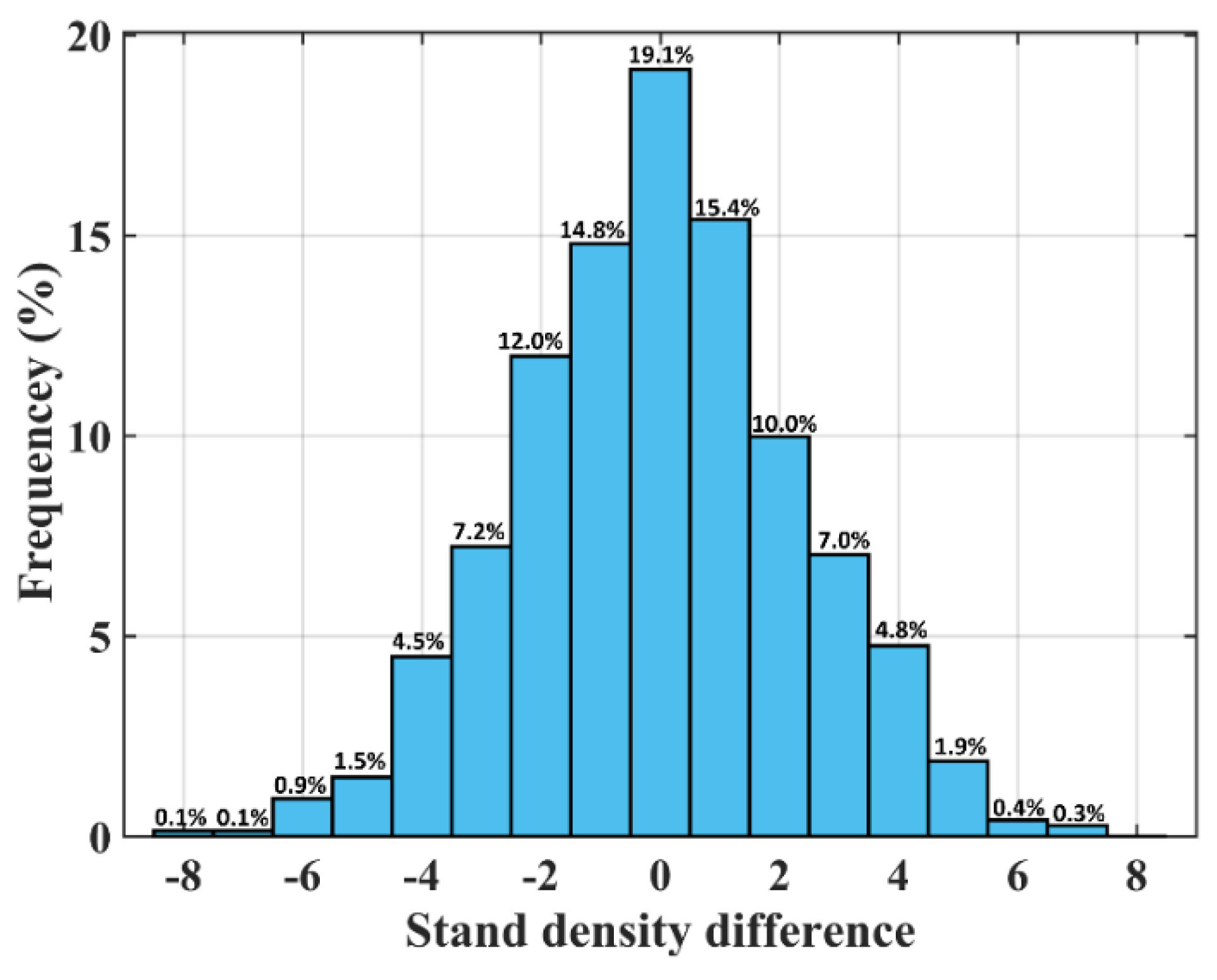
Figure 7.
Boxplot distribution of and values under different laser pulse densities, using CHMFe as the example. (a) Boxplot distribution of values at Csize = 1 m; (b) Boxplot distribution of values at Csize = 0.5 m; (c) Boxplot distribution of values at Csize = 0.2 m; (d) Boxplot distribution of values at Csize = 1 m; (e) Boxplot distribution of values at Csize = 0.5 m; (f) Boxplot distribution of values at Csize = 0.2 m. The black dotted line indicates the distribution range of .


Table 1.
The error assessment results of stand density from the local maximum method. The star (★) marks the minimum for each CHM data type (CHMFe, CHMLe, or CHMHFe) with different Csize values (1, 0.5, or 0.2 m).
Table 1.
The error assessment results of stand density from the local maximum method. The star (★) marks the minimum for each CHM data type (CHMFe, CHMLe, or CHMHFe) with different Csize values (1, 0.5, or 0.2 m).
| Data | CHMFe (Csize: 1 m) | CHMFe (Csize: 0.5 m) | CHMFe (Csize: 0.2 m) | ||||||||||
| 3 | 5 | 7 | 3 | 5 | 7 | 3 | 5 | 7 | 9 | 11 | 13 | 15 | |
| 161 | 61 | 31 | 485 | 182 | 99 | 2432 | 694 | 381 | 246 | 184 | 140 | 102 | |
| 0.04 | 0.00 | 0.00 | 0.60 | 0.07 | 0.00 | 0.92 | 0.72 | 0.50 | 0.26 | 0.08 | 0.01 | 0.00 | |
| 0.21 | 0.69 | 0.83 | 0.02 | 0.14 | 0.50 | 0.00 | 0.01 | 0.03 | 0.07 | 0.14 | 0.30 | 0.48 | |
| 2.00 ★ | 4.34 | 5.36 | 10.20 | 1.68 ★ | 3.18 | 73.47 | 17.39 | 6.98 | 2.96 | 1.73 ★ | 2.30 | 3.17 | |
| Data | CHMLe (Csize: 1 m) | CHMLe (Csize: 0.5 m) | CHMLe (Csize: 0.2 m) | ||||||||||
| 3 | 5 | 7 | 3 | 5 | 7 | 3 | 5 | 7 | 9 | 11 | 13 | 15 | |
| 232 | 104 | 49 | 775 | 314 | 169 | 3504 | 1369 | 750 | 465 | 334 | 248 | 193 | |
| 0.21 | 0.02 | 0.00 | 0.75 | 0.38 | 0.10 | 0.94 | 0.86 | 0.74 | 0.58 | 0.42 | 0.26 | 0.11 | |
| 0.07 | 0.48 | 0.75 | 0.00 | 0.02 | 0.23 | 0.00 | 0.00 | 0.00 | 0.01 | 0.02 | 0.06 | 0.13 | |
| 2.56 ★ | 3.48 | 4.90 | 18.56 | 4.53 | 2.43 ★ | 108.5 | 37.17 | 17.53 | 8.88 | 4.90 | 2.95 | 1.94 ★ | |
| Data | CHMHFe (Csize: 1 m) | CHMHFe (Csize: 0.5 m) | CHMHFe (Csize: 0.2 m) | ||||||||||
| 3 | 5 | 7 | 3 | 5 | 7 | 3 | 5 | 7 | 9 | 11 | 13 | 15 | |
| 140 | 56 | 32 | 449 | 187 | 95 | 2203 | 700 | 403 | 268 | 186 | 142 | 113 | |
| 0.04 | 0.00 | 0.00 | 0.57 | 0.10 | 0.00 | 0.91 | 0.72 | 0.52 | 0.31 | 0.12 | 0.02 | 0.01 | |
| 0.32 | 0.72 | 0.84 | 0.01 | 0.15 | 0.52 | 0.00 | 0.01 | 0.01 | 0.06 | 0.17 | 0.29 | 0.43 | |
| 2.58 ★ | 4.53 | 5.32 | 8.95 | 2.19 ★ | 3.50 | 65.36 | 16.98 | 7.53 | 3.71 | 2.51 | 2.43 ★ | 3.04 | |
Table 2.
The test data errors () and obtained when using the LOOCV method.
| Data | CHMFe (Csize: 1 m) | CHMFe (Csize: 0.5 m) | CHMFe (Csize: 0.2 m) | ||||||||||
| 3 | 5 | 7 | 3 | 5 | 7 | 3 | 5 | 7 | 9 | 11 | 13 | 15 | |
| 0.01 | 0.11 | 0.43 | 0.07 | 0.02 | 0.09 | 0.07 | 0.01 | 0.05 | 0.09 | 0.04 | 0.14 | 0.13 | |
| 3.52 | 5.69 | 10.78 | 4.48 | 6.01 | 4.95 | 7.24 | 6.13 | 7.41 | 5.3 | 6.6 | 7.71 | 4.45 | |
| 1.48 | 1.98 | 2.66 | 1.78 | 1.24 | 1.4 | 2.08 | 1.71 | 1.5 | 1.87 | 1.62 | 1.97 | 1.66 | |
| 1.89 | 2.36 | 3.36 | 2.19 | 1.79 | 1.8 | 2.65 | 2.17 | 2.15 | 2.36 | 2.25 | 2.41 | 2.02 | |
| Data | CHMLe (Csize: 1 m) | CHMLe (Csize: 0.5 m) | CHMLe (Csize: 0.2 m) | ||||||||||
| 3 | 5 | 7 | 3 | 5 | 7 | 3 | 5 | 7 | 9 | 11 | 13 | 15 | |
| 0.13 | 0.01 | 0.45 | 0.14 | 0.05 | 0.09 | 0.03 | 0.04 | 0.08 | 0.01 | 0.1 | 0.27 | 0.04 | |
| 6.38 | 8.07 | 14.93 | 5.7 | 5.49 | 7.39 | 5.67 | 4.79 | 5.96 | 5.6 | 6.12 | 6.58 | 4.9 | |
| 2.11 | 3.34 | 4.12 | 1.85 | 2.14 | 2.2 | 2.05 | 1.9 | 1.86 | 2.07 | 1.98 | 2.36 | 1.85 | |
| 2.6 | 3.88 | 4.91 | 2.34 | 2.67 | 2.85 | 2.59 | 2.26 | 2.3 | 2.44 | 2.47 | 2.91 | 2.28 | |
| Data | CHMHFe (Csize: 1 m) | CHMHFe (Csize: 0.5 m) | CHMHFe (Csize: 0.2 m) | ||||||||||
| 3 | 5 | 7 | 3 | 5 | 7 | 3 | 5 | 7 | 9 | 11 | 13 | 15 | |
| 0.14 | 0.01 | 0.32 | 0.05 | 0.02 | 0.14 | 0.08 | 0.15 | 0.15 | 0.03 | 0.01 | 0.01 | 0.01 | |
| 12.65 | 6 | 8.81 | 6.9 | 5.84 | 6.75 | 5.29 | 4.84 | 5 | 7.23 | 6.65 | 6.44 | 5.09 | |
| 2.03 | 2.39 | 3.73 | 1.71 | 1.85 | 2.09 | 1.94 | 1.86 | 1.58 | 1.84 | 1.85 | 1.82 | 1.83 | |
| 3.08 | 2.8 | 4.94 | 2.19 | 2.43 | 2.65 | 2.34 | 2.26 | 1.92 | 2.43 | 2.52 | 2.39 | 2.28 | |
Table 3.
The error assessment results using regression models to correct stand density errors from three types of CHM (CHMFe, CHMLe, and CHMHFe) and three kinds of Csize (1, 0.5, and 0.2 m).
Table 3.
The error assessment results using regression models to correct stand density errors from three types of CHM (CHMFe, CHMLe, and CHMHFe) and three kinds of Csize (1, 0.5, and 0.2 m).
| Data | CHMFe (Csize: 1 m) | CHMFe (Csize: 0.5 m) | CHMFe (Csize: 0.2 m) | ||||||||||
| 3 | 5 | 7 | 3 | 5 | 7 | 3 | 5 | 7 | 9 | 11 | 13 | 15 | |
| −0.07 | 0.01 | −0.02 | −0.22 | −0.08 | −0.01 | −0.75 | −0.19 | −0.11 | −0.06 | −0.04 | −0.04 | 0.00 | |
| 1.58 | 0.32 | 0.32 | 4.59 | 1.74 | 0.71 | 18.48 | 5.56 | 3.08 | 1.87 | 1.40 | 1.12 | 0.54 | |
| −1.55 | −0.29 | −0.24 | −3.28 | −1.58 | −0.84 | −5.20 | −3.99 | −2.28 | −1.33 | −0.91 | −0.82 | −0.30 | |
| 0.18 | 0.16 | 0.21 | 0.20 | 0.15 | 0.12 | 0.24 | 0.19 | 0.17 | 0.18 | 0.17 | 0.23 | 0.14 | |
| 0.15 | 0.17 | 0.21 | 0.15 | 0.10 | 0.11 | 0.14 | 0.12 | 0.11 | 0.12 | 0.11 | 0.14 | 0.14 | |
| 2.40 | 2.18 | 2.83 | 2.60 | 2.17 | 1.74 | 2.91 | 2.64 | 2.60 | 2.56 | 2.60 | 3.14 | 1.90 | |
| Data | CHMLe (Csize: 1 m) | CHMLe (Csize: 0.5 m) | CHMLe (Csize: 0.2 m) | ||||||||||
| 3 | 5 | 7 | 3 | 5 | 7 | 3 | 5 | 7 | 9 | 11 | 13 | 15 | |
| −0.09 | −0.04 | 0.00 | −0.33 | −0.15 | −0.07 | −1.74 | −0.63 | −0.27 | −0.21 | −0.16 | −0.16 | −0.11 | |
| 1.78 | 0.74 | 0.15 | 6.29 | 2.55 | 1.18 | 31.47 | 11.32 | 5.55 | 3.88 | 2.95 | 2.53 | 1.89 | |
| 0.33 | 0.23 | 0.55 | −0.20 | 0.59 | 0.83 | −8.88 | 0.01 | 0.60 | −0.20 | −0.73 | −0.97 | −0.78 | |
| 0.19 | 0.29 | 0.35 | 0.17 | 0.17 | 0.21 | 0.21 | 0.19 | 0.16 | 0.16 | 0.17 | 0.17 | 0.14 | |
| 0.16 | 0.18 | 0.17 | 0.15 | 0.15 | 0.15 | 0.16 | 0.12 | 0.15 | 0.16 | 0.12 | 0.12 | 0.10 | |
| 2.53 | 3.56 | 4.88 | 2.42 | 2.35 | 2.82 | 2.76 | 2.37 | 2.17 | 2.19 | 2.12 | 2.02 | 1.76 | |
| Data | CHMHFe (Csize: 1 m) | CHMHFe (Csize: 0.5 m) | CHMHFe (Csize: 0.2 m) | ||||||||||
| 3 | 5 | 7 | 3 | 5 | 7 | 3 | 5 | 7 | 9 | 11 | 13 | 15 | |
| −0.04 | 0.01 | 0.00 | −0.12 | −0.09 | −0.03 | −0.82 | −0.18 | −0.14 | −0.13 | −0.07 | −0.05 | −0.04 | |
| 1.04 | 0.16 | 0.10 | 3.49 | 1.79 | 0.78 | 18.26 | 5.05 | 3.46 | 2.58 | 1.74 | 1.28 | 1.03 | |
| −0.38 | 0.14 | 0.19 | −2.03 | −1.21 | −0.53 | −8.28 | −1.56 | −2.57 | −1.92 | −1.54 | −0.91 | −0.99 | |
| 0.23 | 0.20 | 0.28 | 0.19 | 0.18 | 0.25 | 0.22 | 0.20 | 0.17 | 0.18 | 0.21 | 0.21 | 0.22 | |
| 0.16 | 0.11 | 0.17 | 0.13 | 0.18 | 0.16 | 0.14 | 0.14 | 0.13 | 0.15 | 0.17 | 0.16 | 0.17 | |
| 3.47 | 2.24 | 3.71 | 2.71 | 2.59 | 3.45 | 2.69 | 2.55 | 2.39 | 2.59 | 3.04 | 2.92 | 3.00 | |
Table 4.
Results of stand density estimation obtained from other studies. The minimum (trees/100 m2) values were selected and denoted by * if the study reported multiple results.
Table 4.
Results of stand density estimation obtained from other studies. The minimum (trees/100 m2) values were selected and denoted by * if the study reported multiple results.
| Study | Remote Sensing Data | Forest Type | |
|---|---|---|---|
| This study | airborne LiDAR (Optech ALTM 3070) | tropical forest | 1.68 * |
| Lee and Lucas [40] | airborne LiDAR (Optech ALTM 1020) | white cypress pine | 1.33 * |
| Palace, et al. [41] | terrestrial LiDAR (FARO Focus 3D) | tropical forest | 1.53 * |
| Kahriman, et al. [42] | optical satellite (Landsat TM) | pine and beech | 0.83 * |
| Chrysafis, et al. [43] | optical satellite (Landsat 8 OLI) | black pine and oaks | 2.57 * |
| Mohammadi, et al. [44] | optical satellite (Landsat ETM+) | hornbeam and oak | 1.70 * |
| Wang and Qi [45] | SAR satellite (JERS-1) | deciduous forests | 1.61 |
© 2018 by the authors. Licensee MDPI, Basel, Switzerland. This article is an open access article distributed under the terms and conditions of the Creative Commons Attribution (CC BY) license (http://creativecommons.org/licenses/by/4.0/).
Share and Cite
MDPI and ACS Style
Lee, C.-C.; Wang, C.-K. Estimating Stand Density in a Tropical Broadleaf Forest Using Airborne LiDAR Data. Forests 2018, 9, 475. https://doi.org/10.3390/f9080475
AMA Style
Lee C-C, Wang C-K. Estimating Stand Density in a Tropical Broadleaf Forest Using Airborne LiDAR Data. Forests. 2018; 9(8):475. https://doi.org/10.3390/f9080475
Chicago/Turabian StyleLee, Chung-Cheng, and Chi-Kuei Wang. 2018. "Estimating Stand Density in a Tropical Broadleaf Forest Using Airborne LiDAR Data" Forests 9, no. 8: 475. https://doi.org/10.3390/f9080475
Note that from the first issue of 2016, this journal uses article numbers instead of page numbers. See further details here.