Effects of Tree Trunks on Estimation of Clumping Index and LAI from HemiView and Terrestrial LiDAR


1
Beijing Institute of Space Mechanics and Electricity, No. 104, Road Youyi, Beijing 100094, China
2
State Key Laboratory of Remote Sensing Science, Institute of Remote Sensing and Digital Earth, Chinese Academy of Sciences, Beijing 100101, China
3
CAVELab Computational and Applied Vegetation Ecology, Faculty of Bioscience Engineering, Ghent University, 9000 Ghent, Belgium
*
Author to whom correspondence should be addressed.
Forests 2018, 9(3), 144; https://doi.org/10.3390/f9030144
Submission received: 25 January 2018
/
Revised: 7 March 2018
/
Accepted: 13 March 2018
/
Published: 16 March 2018
(This article belongs to the Special Issue Remote Sensing of Leaf Area Index (LAI) and Other Vegetation Parameters)
Abstract
:Estimating clumping indices is important for determining the leaf area index (LAI) of forest canopies. The spatial distribution of the clumping index is vital for LAI estimation. However, the neglect of woody tissue can result in biased clumping index estimates when indirectly deriving them from the gap probability and LAI observations. It is difficult to effectively and automatically extract woody tissue from digital hemispherical photos. In this study, a method for the automatic detection of trunks from Terrestrial Laser Scanning (TLS) data was used. Between-crown and within-crown gaps from TLS data were separated to calculate the clumping index. Subsequently, we analyzed the gap probability, clumping index, and LAI estimates based on TLS and HemiView data in consideration of woody tissue (trunks). Although the clumping index estimated from TLS had better agreement (R2 = 0.761) than that from HemiView, the change of angular distribution of the clumping index affected by the trunks from TLS data was more obvious than with the HemiView data. Finally, the exclusion of the trunks led to a reduction in the average LAI by ~19.6% and 8.9%, respectively, for the two methods. These results also showed that the detection of woody tissue was more helpful for the estimation of clumping index distribution. Moreover, the angular distribution of the clumping index is more important for the LAI estimate than the average clumping index value. We concluded that woody tissue should be detected for the clumping index estimate from TLS data, and 3D information could be used for estimating the angular distribution of the clumping index, which is essential for highly accurate LAI field measurements.
1. Introduction
Leaf area index (LAI) is an important factor in describing ecosystem structure and function. It not only relates to photosynthetic and respiration activities, but also plays a dominant role in the reflectance characteristics of vegetated land surfaces [1]. In many studies, passive optical remote sensing images from satellites and airborne platforms have been used to retrieve LAI [2,3,4]. Light Detection and Ranging (LiDAR) is an active optical sensing technique and offers an alternative to estimate forest structure in 3D. It has therefore been widely used to estimate forest structure parameters [5,6,7,8,9], especially the LAI parameters [10,11,12,13,14,15].
However, the calibration of satellite-based and airborne-based LAI maps requires adequate ground truth points. The fast and accurate extraction of canopy structure parameters in the field is very important for ground-based LAI estimates, which are important to evaluate the accuracy of airborne LAI estimates. However, in some studies, the LAI has often been replaced with the retrieved plant area index (PAI), which includes the leaf area index, wood area index, and other component area indices. This does not benefit the validation of retrieval results from satellite images. Currently, ground-based LAI measurements can be performed through two major techniques: direct and indirect measurements [16,17]. Direct (Destructive) LAI determination is not compatible with long-term monitoring of the spatial and temporal dynamics of leaf area development [18]. Optical indirect techniques are the methods most commonly used in validation studies due to the speed and ease of LAI measurements over large areas. Optical techniques are based on the measurements of light transmittance through canopies [17,19] and have been implemented using multiple commercial optical instruments including the LAI-2000 plant canopy analyzer (LI-COR, Lincoln, NE, USA), AccuPAR (Decagon Devices, Inc., Pullman, WA, USA), Tracing radiation and Architecture of Canopies system (TRAC, 3rd Wave, Nepean, Ontario, Canada), and digital hemispherical photographs [17]. The accuracy of these indirect LAI measurements is often limited by leaf clumping, woody-to-total area ratio, and illumination conditions.
The clumping effect is an important factor complicating indirect LAI measurements. This index at different scales quantifies the spatial pattern of leaf distribution and is a transforming factor for calculating the true LAI from the effective LAI. However, the estimation of the clumping index can be affected by woody material. There are typically two types of clumping index retrieval methods: the finite length averaging method (hereafter LX) [20], and the gap size distribution method (hereafter CC) [21]. Due to the limitations of the two methods [22,23], a new method was developed by combining the gap size distribution and logarithmic methods for LAI estimation (hereafter CLX) [23]. However, the clumping index results from the three methods notably differ. The CC method does not show radical changes of the clumping index value outside zenith angles ranging from 30° to 60°, which is in contrast to the other two methods. Based on hemispherical photography, the clumping index increases with the view zenith angle in both boreal and temperate forests [23,24,25]. Although the angular dependence of clumping is an important characteristic in determining the clumping index, a limited number of clumping indices have been estimated within a narrow and moderate range of zenith angles including 30–80°, 54–63° and 57.5° [24,26,27]. Given the different ranges of the view zenith angle, different clumping index values were retrieved from three instruments in an open savanna ecosystem using the same methods as CLX or CC [28]. This indicates that estimating the angular distribution of the clumping index from hemispherical photography within a stand level remains challenging [23,28]. Meanwhile, several clumping index values covering a wide range of view zenith angles are required to calculate hemispherical average clumping index values, where the clumping index changes depending on the view zenith angle [28]. To quantify and interpret the clumping index of the forest canopy, several questions need to be addressed including the range of the view zenith angle and how the clumping index changes with the view zenith angle. Additionally, during LAI retrieval, gap probability and clumping index estimates are affected by the quantity of woody tissue. For deciduous forests, the wood area index is generally estimated during leafless periods and subtracted from the total PAI [29]. However, this method is not suitable for coniferous forests. Although the contribution of woody tissue to gap probability and LAI estimation is obvious, it remains undetermined in the case of indirect measurements in coniferous forests [30]. This problem is even bigger in Mediterranean forests or other semi-arid forests where trees and shrubs usually have small leaves and the importance of trunks should be proportionally more important. A few studies have aimed to quantify the effect of woody tissue on the gap probability and clumping index estimation by developing an image analysis approach [31,32], which can still be affected by imaging conditions and image processing techniques.
Terrestrial Laser Scanning (TLS) has been used as an active optical sensing tool to estimate forest structure parameters from field measurements [9,33]. 3D space information from TLS is useful for the estimation of gap distribution and tree structure. Recent studies have proven that TLS offers high performance estimates of gap probability and LAI [22,34,35]; however, very few studies have addressed the impact of the clumping index in these LAI estimates. Moorthy et al. (2011) calculated the clumping index using TLS data based on the CC method and an obvious improvement in LAI estimates was achieved in comparison to field estimates from LAI-2000 [36]. The clumping index was estimated by using the gap size information derived from images of gap probabilities yielded by the Echidna Validation Instrument (EVI), which is a TLS method with dual wavelengths [24]. The TLS scanner can produce a ‘pseudo’ Normalized Difference Vegetation Index (NDVI) image, which is beneficial for the detection of woody material. In their study [24], woody structures were considered in clumping index estimates and identified using a threshold of the ratio of total power to reflected pulse width. García et al. evaluated the potential of TLS to estimate the clumping index in different vegetation types based on the spatial distribution of the returns, the gap distribution and the gap size distribution, and proved that TLS data could be used to estimate the clumping index [37]. Given the importance of the spatial distribution of the clumping index, the angular distribution of woody tissue and its effect on the spatial distribution of the clumping index needs to be estimated. Meanwhile, most of the woody tissue is trunk, which has a greater effect on the clumping index than other components. To solve this problem, we introduced a method that could be used to exclude the trunk from terrestrial LiDAR data and we analyzed the influence of the trunk on the gap probability, clumping index, and LAI at all view zenith angles.
In this study, we first extracted the tree trunk point clouds from terrestrial LiDAR data. Within-crown and between-crown gap probabilities were calculated to estimate the clumping index and LAI. The angular dependence of the gap probability, clumping index, and LAI were analyzed before and after the exclusion of tree trunks. At the same time, we compared the performance of TLS with that of digital hemispherical photos with respect to the angular distribution of the clumping index and LAI and the analysis of trunk effects. We addressed the following research questions: (1) How does the clumping index change within the whole range of view zenith angles? (2) How strong is the influence of tree trunks on the canopy gap probability, clumping index, and LAI at different view zenith angles? (3) How different are the canopy gap probability, clumping index, and LAI estimates derived from TLS data and HemiView photos?
2. Materials
2.1. Study Area Description
The study area is located in the Qilian Mountains within the Gansu Province in Western China (38°19′–38°29′ N, 100°12′–100°20′ E), as shown in Figure 1. The elevation varies from 2500 to 3800 m above sea level. This area is cold and dry with low precipitation and presents the typical features of a temperate continental mountainous climate. The atmospheric circulation in this area is controlled by the Mongolia anticyclone in winter. Influenced by climate and terrain, the prevalent vegetation types in the study area are mountainous pastures and forests. The dominant vegetation types include two tree species, the Qinghai Spruce (Picea crassifolia Kom.) and Qilian Juniper (Sabina przewalskii Kom.), as well as grassland. The vegetation density varies depending on the terrain, soil, water, and climate factors. In this study, the coniferous tree species Qinghai spruce was selected as the study object.
2.2. Sampling Design and Field Measurements
A 100 × 100 m sample plot was selected in the study area. The plot was selected as the major area for field measurements (Figure 1). The ground in the plot was relatively flat with a slope of about five degrees. The plot was dominated by the same tree species, the Qinghai spruce. This plot was divided into 16 subplots, with each subplot having a size of 25 × 25 m. Measurement points were located in the center of each subplot (Figure 2) and TLS and HemiView (Delta-T devices Ltd., Cambridge, UK) were used to acquire data at the 13 subplots (red solid circles in Figure 1).
The terrestrial laser scanner RIEGL LMS-Z360i (RIEGL, Horn, Austria) was used in this study. The configuration of RIEGL LMS-Z360i used in the field is shown in Table 1. The scanner is based on the principle of time-of-flight measurement with short infrared laser pulses (900 nm). The first and last returns could be recorded, and the first returns of points were used in our study. When the laser scanner was vertically mounted on a tripod located at the center of the subplot, the vertical range of scanning (line scanning angle) was −50°~40° and the horizontal range of scanning (frame scanning angle) was 360° (Table 1) The vertical angle of 40°~90° needed to be obtained by tilt scanning of TLS at the same position to cover the upper hemisphere view. The TLS data from the vertical and tilt scan at the same position were used for the detection of trunks and the estimation of gap probability in the study. Figure 2 shows the intensities obtained using the vertical and tilt mounts of the terrestrial laser scanner.
In addition, orientation information can be acquired using a compass and spirit level. Three angles of the vertical and tilt scans were obtained using this method including the roll, pitch, and yaw angle. A compass was employed to orient the vertical and tilt scans of the laser scanner and to measure the yaw angle around the scanner’s Z-axis. The roll angle of the X-axis of the scanner and the pitch angle of the Y-axis of the scanner were determined with an electronic spirit level. As the intersection angle between the vertical and tilt mount was 90°, we obtained a tilt mount calibration matrix from the three angles based on the method in [38]. The data acquired at the tilt mount can be transformed into its corresponding vertical mount coordinates using the tilt mount calibration matrix.
We took hemispherical photographs as field samples using HemiView (Delta-T Device, Cambridge, UK) including a self-levelling mount and a Nikon Coolpix 8400 with FC-E9 adapter lens (Nikon, Tokyo, Japan). The camera and lens were mounted and levelled with a bubble level before use. The measurements were performed under overcast conditions or conditions of diffuse skylight. A hemispherical photograph provides a permanent record and is a valuable source of information for canopy gaps. The photographs were processed with digital hemispherical photography (DHP) software to derive the effective LAI. Hemispherical photographs were acquired at a height of 0.8 m for each station in this plot. An example is shown in Figure 3. Similar to the case of the terrestrial LiDAR, the measurement locations in the plot are shown in Figure 1.
3. Methods
3.1. Gap Probability Theory
Beer’s Law, which relates the absorption of light to the properties of particles [39], was used to relate the LAI to the gap probability of the canopy. The original formulation of Beer’s Law assumes the random distribution of light-intercepting elements in the pathway of penetrating beams. However, leaves in natural forest canopies are clumped within crowns instead of being randomly distributed. Therefore, Nilson introduced the clumping index to the relationship between the LAI and gap probability [40]:
where θ is the view zenith angle; G(θ) is the leaf projection function, namely the G-function, which quantifies the projection coefficient of unit foliage area on a plane perpendicular to the view direction [41]; and is the clumping index, which quantifies the degree of the deviation of foliage spatial distribution from the random case, and it is a value between 0 and 1 (the higher value denotes less clumping degree). Le and L are the effective LAI and true LAI, respectively. Random distribution of the elements (no clumping) was assumed for the retrieval of Le while L could be calculated after the clumping index was taken into account. In fact, L refers to the plant area index, which includes the LAI and wood area index if it has not been corrected for the influence of woody tissue on P(θ). Although several instruments have been used to perform clumping index retrievals such as the Tracing Radiation and Architecture of Canopies (TRAC) instrument, hemispherical photography, and Echidna Validation Instrument [24], the effect of woody tissue on the clumping index and LAI needs to be accounted for. In this study, we compared the results from the HemiView data with those from the TLS data with and without woody tissue.
3.2. HemiView
An important step in measuring the clumping index of forests is the separation of between-crown gaps from within-crown gaps. To derive the gap fraction from hemispherical images, each image must be separated into areas of gaps and plant tissue using an image classification algorithm. The mean gap probability can be obtained by dividing the average number of pixels of all gaps () by the total number of pixels A of each image at each view zenith angle. Thus, the effective LAI is calculated by:
A method was proposed for calculating the clumping index from digital cover photography (DCP), which offers the advantage of separately determining different gaps in the canopy including between-crown and within-crown gaps [32]. The between-crown gap probability can be derived from the average number of pixels of the between-crown gap and the total number of pixels . at each view zenith angle. Therefore, the LAI can be calculated when the clumping effect can be considered explicitly [32,42]:
where is the crown cover; and is the average number of pixels of the larger gap of the image, which is generally the gap between adjacent crowns. The calculation of the clumping index is as follows:
Based on the above-mentioned methods, we should successively retrieve the gap probability, clumping index, and LAI. However, before retrieving the gap probability, it is essential to extract the tree trunks and between-crown gaps from the images. The separation was performed using Adobe Photoshop and digital hemispherical photography (DHP) software. The shape features of objects can be used to identify the trunk tissue in an image. The separation of the trunk area from other elements of trees in this study was conducted with object-based image analysis using the eCognition software (Trimble, Munich, Germany) [32]. The advantage of this method is that it allows for the use of object mean values for the image instead of separately applying a threshold to each pixel. The threshold values for trunk tissue detection depend on the object size classes. Objects were only classified as trunk tissue when they were not obscured by leaves.
The gaps were classified using thresholds of the object’s average brightness and blue difference [32]. Hemispherical photos were analyzed using Adobe Photoshop 10 (Adobe, San Jose, CA, USA) to separate the between-crown and within-crown gaps as follows: large gaps between the tree crowns in each photo were selected using the ‘Magic wand’ tool with the SHIFT key held down and the total number of pixels of large gaps was recorded using the histogram. Then, the hemispherical sphere was divided into segments along the zenithal and horizontal directions separately using DHP software. The mean gap probability and between-crown gap probability of ten view zenith angles (θ = 4.5°, 13.5°, 22.5°, …, 85.5°) were then calculated based on the DHP software. Subsequently, the clumping index and LAI were derived based on Equations (3) and (4).
In addition to the analysis of the influence of the trunks on the gap fraction, clumping index, and LAI, the relative bias was used as the evaluation index. The relative biases of the effect on the gap fraction, clumping index, and LAI were defined as:
where Pin(θ), CIin(θ) and Lin(θ) are the gap probability, clumping index, and LAI including trunks, respectively. Here, Pex(θ), CIex(θ) and Lex(θ) are the gap probability, clumping index, and LAI excluding trunks, respectively.
3.3. Terrestrial Laser Scanner
3.3.1. Gap Probability Calculation
The directional canopy gap fraction was obtained from the data of a terrestrial laser scanner [33]. The gap fraction was derived from the terrestrial laser scanner data based on the ratio of the number of laser beams passing through the canopy to the total number of beams emitted into the canopy. A laser scanner model was developed to determine the number and direction of all shots in a scan [43]. The interception of laser beams and objects can be expressed as polar coordinates (r, θ, ϕ), which can be determined by the range, zenith angle θ, and azimuth angle ϕ. We subdivided the view zenith and azimuth angles based on the minimum resolution angle of the laser scanner. The view zenith angle θ (from 0° to 90°) was divided into . subangles and the azimuth angle ϕ (from 0° to 360°) was divided into subangles. If a laser beam did not intercept an object, the gap fraction of the angle voxel was ‘1’; if the laser beam intercepted an object, the gap fraction of the angle voxel was ‘0’.
In addition, the forest canopy structure was reconstructed using a 3D arrangement of voxels created from all LiDAR shots and the gap fraction was calculated from the voxels [44]. The gap fraction of each 5° zenith angle was calculated as:
where k is the number of divisions from 1 to 18; and P(θk) is the mean gap fraction of each 5° zenith angle. The azimuth angle was divided into 360 1° steps and the view zenith angle from 0° to 90° was divided into 18 5° steps.
3.3.2. Between-Crown Gap Separation
To estimate the clumping index and LAI, between-crown gaps were separated from within-crown gaps. As the TLS records the gap fraction and distance of objects in each direction, LiDAR data at different distances were processed for calculating the gap fraction, and it was possible to distinguish within-crown and between-crown gaps based on the change in size and distance of connected gap segments. Between-crown gaps consist of many large connected gaps, which form relatively large and open spaces. In contrast, within-crown gaps are broken gaps that are distributed among canopy leaves and disconnected. The change of large connected gaps was analyzed from the farthest to the nearest distance. If the size of the connected gap remained unchanged at all distances, the path lengths of the laser beams did not intercept any leaves. With reference to Zhao et al.’s method [24], a threshold value was chosen to identify between-crown gaps and how they changed with distance:
where l is the distance at which a single laser beam arrives; dθ is the beam divergence for a single laser beam; and n is an integer number.
If the area of the gap fraction was larger than the threshold value, the gap was classified as a between-crown gap. If it was smaller than the threshold value, the gap was considered to be a within-crown gap. Once the between-crown gaps were distinguished from the within-crown gaps, the corresponding total gap fractions and between-crown gap fractions for each zenith angle could be calculated.
3.3.3. Clumping Index Calculation
The effective LAI can be described using Equation (1). If only the total gap probability within gaps is known, the assumption must be tailored to randomly distributed leaf elements. The effective LAI can be derived from:
where is the canopy mean gap probability, which can be estimated from terrestrial LiDAR point cloud data [33].
After separating the between-crown gap probability using the method described in Section 3.3.2, the LAI can be calculated using a method similar to that used in [32,39]:
where is the between-crown gap probability.
Hence, the clumping index can be directly calculated by dividing the effective LAI by the true LAI:
3.3.4. Trunk Detection
To estimate the impact of woody tissue (trunk) on the LAI, the point cloud returned from tree trunks should first be identified. The central idea is that there are many points on the trunk surface towards the TLS and that no point is on the opposite side due to the shading effect of trunks [45]. When the laser scans the trunk of a tree, the laser shots are occluded by the trunk with no points in the longer range. The detailed algorithm for the identification of tree trunks can be described as follows. First, we identified the ‘trunk angle’ along the azimuth direction based on these characteristics (as shown in Figure 4). We defined the trunk angle as a range of angles within which the trunk point cloud between ground and a height of 1.3 m occurs when they are projected in the x-y plane. In a plot with 25 m × 25 m size, we searched for points from far away to near the azimuth angle and saved this angle if there were no points beyond a certain distance. Second, after identifying the ‘trunk angle’, we extracted the points in this range of the ‘trunk angle’ from all points based on the azimuth angles. Finally, we confirmed the positions of the trunks based on the point density in vertical direction by setting a threshold to remove other non-trunk points. The threshold value could be established based on the points’ distance and configuration of the laser scanner. This way, we could extract the point cloud of the tree trunks based on the ‘trunk angle’ characteristics. However, leaves obscured by the trunk should be considered in the calculation of LAI. We assumed that the distribution of the obscured leaves was the same as the distribution of the other leaves. We then calculated the mean gap fraction for each view zenith angle after removing the point cloud of the trunks. The clumping index and LAI were also retrieved from the TLS data.
To analyze the effect of trunks on the gap fraction, clumping index, and LAI based on TLS data and compare them with results from the HemiView data, the relative biases were calculated using Equation (5) and interpolated with several angles from HemiView.
4. Results and Discussion
4.1. Canopy Gap Fraction Distribution
The terrestrial laser scanner data of our sample plots were selected to evaluate their potential for the estimation of gap fractions. For a comparison with the results from the HemiView, twenty of the directional gap fractions within each 5° from the TLS were averaged as the single gap fraction value for the corresponding angle from 0° to 90°. As shown in Figure 5, the gap fractions derived from the hemispherical photography and terrestrial laser scanner showed good consistency, but the latter was lower than the former in the zenith angle range from 10° to 70°. We found that the gap probabilities from TLS and HemiView were affected by the trunks and increased after excluding them. The detailed results of the effect will be analyzed in Section 4.4. Based on Figure 5b, the trunks had a greater effect at some view zenith angles (from 15° to 55°) than at other zenith angles for HemiView, while the trunks at most view zenith angles had a similar effect on the gap probabilities for TLS. Due to the active TLS detection technique, we could automatically identify trunks from point cloud data and remove them. However, we could not determine if other trees were located behind the identified trunks from the LiDAR data. Therefore, the gap probabilities at most view zenith angles changed after removing the trunks from the point cloud. For HemiView, Photoshop and DHP software were used to process photos, then the trunk pixels could be manually selected based on the background of sky light (Figure 3). At small view zenith angles, the trunks are too thin to be identified from bright background. Furthermore, it is also difficult to determine if there is another tree located behind the identified trunks at larger view zenith angles due to the dense forest background. Therefore, the trunk surface area at these angles, to a large part, could not be removed.
4.2. Clumping Index
In general, the estimated clumping indices increased with increasing view zenith angle (Figure 6). The clumping index significantly changed at larger view zenith angles after removing the trunk points from the point cloud. This indicated that the influence of the trunks on the clumping index was smaller at smaller view zenith angles than at larger angles. For HemiView, the effect of trunks on the clumping index between 30° and 70° was about 10–30% more than at other angles (Figure 6b), which was similar to the influence on the gap probability. However, the clumping index decreased with the removal of trunks, which differed from the TLS results. In addition, the clumping index of both TLS and HemiView showed a similar behavior, which was observed in several other studies [23,30]. Rye et al. asserted that heterogeneous ecosystem-scale tree distribution patterns caused different tree clustering at different zenith angles [28]. From the viewpoint of 3D space, the trunk distribution was clumped, not uniform. While projected to 2D images, trunks at larger view zenith angles showed uniformity. Thus, the clumping index from HemiView at larger view zenith angles was higher than at lower view zenith angles and monotonically increased with increasing view zenith angle.
In addition, we also estimated the hemispherical average clumping index from two types of data after removing the trunks (Figure 7). The results obtained using TLS and HemiView were highly correlated (R2 = 0.761). The results also showed that the clumping index results from TLS were higher than those from HemiView in the case of more clumping, while the opposite result was obtained in the case of less clumping. Although good agreement has been achieved between EVI images and hemispherical photos using the 2D image processing method [24], we could be confident that the dimension of data from HemiView and TLS and their processing method also affects the estimation of the clumping index, especially the effect of removing trunks.
4.3. Leaf Area Index
Based on the methods proposed in Section 2, the effective LAI and LAI in the study area were estimated from the TLS data and HemiView images. The angular distributions of LAI from TLS and HemiView have a similar shape (Figure 8); however, the trunks have a 3–25% effect on the LAI, and the effect varies with the view zenith angle. The exclusion of trunks yielded an ~19.6% lower LAI based on the TLS data, while the exclusion of trunks from the HemiView data yielded an ~8.9% lower LAI on average. Due to the exclusion of trunks from the TLS data, both the decrease of the gap probability and increase of the clumping index reduced the estimated LAI value. In contrast, the exclusion of trunks from the HemiView data and the associated decrease of the gap probability reduced the retrieved LAI value and the decrease of the clumping index resulted in a LAI increase. Therefore, the exclusion of trunks had less effect on the LAI from HemiView than on that from TLS. The magnitude of the influence of trunks on the LAI is therefore not only affected by the proportion of tree distribution, but by its patterns and measuring methods. In addition, we compared the effective LAI and LAI of 13 measurement sites derived from TLS with that obtained from HemiView (Figure 9a,b) and found that they had good correlation, though the correlation coefficient of HemiView and TLS decreased from 0.724 to 0.613 after introducing the clumping index. Meanwhile, we found that the results from the TLS data were generally higher than those derived from the HemiView images and we assumed it was due to the higher gap fractions over a 30°–70° view zenith angle determined based on the HemiView data (Figure 5), which was stated in [29].
4.4. Tree Trunk Effects
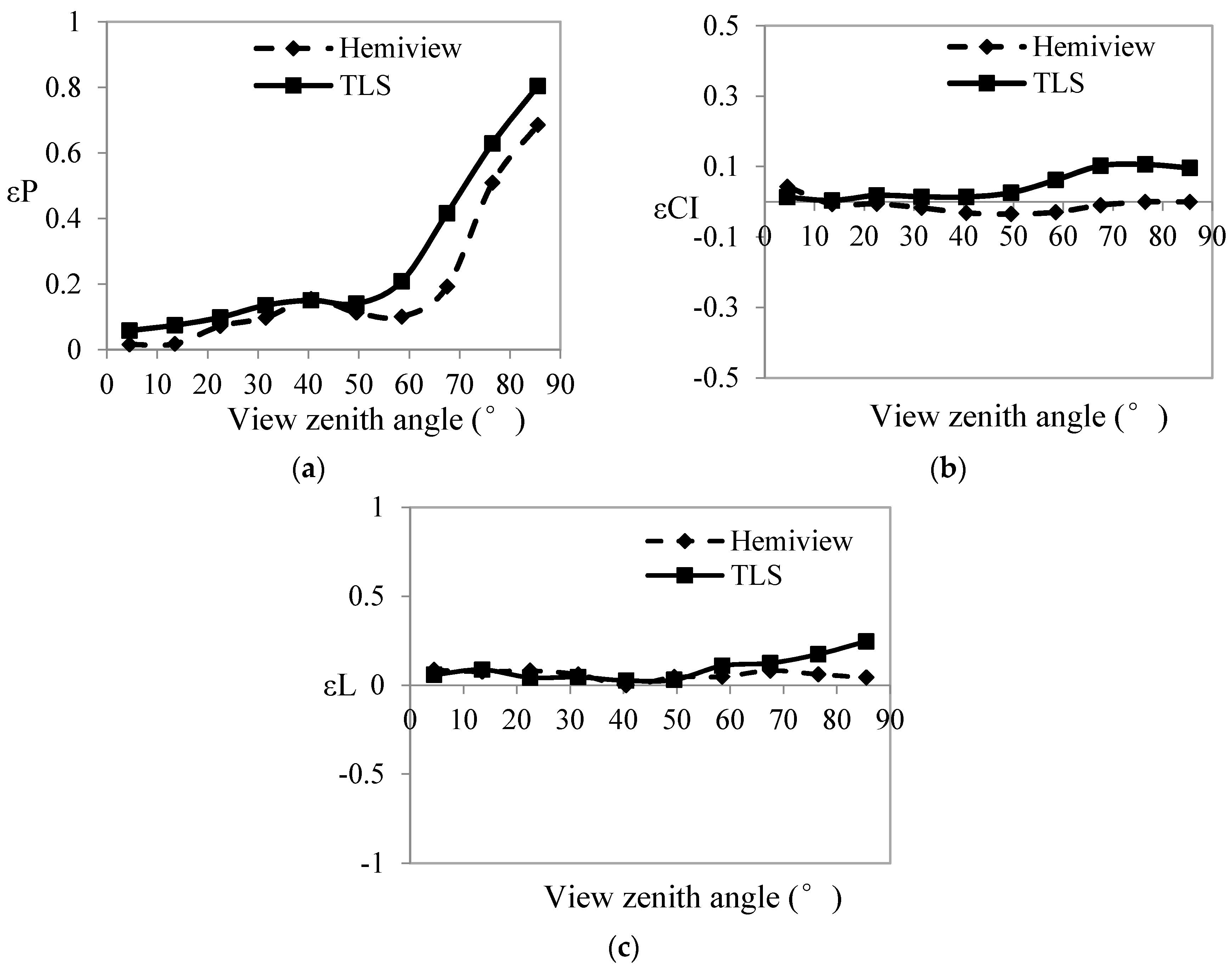
The influence of tree trunks on the gap probability, clumping index, and LAI was analyzed. The effect of the trunks on the gap probability increased with the increasing view zenith angle (Figure 10a). The trunk surface area in the sensor view field increased with the increasing view zenith angle. In this case, εP was <20% when the view zenith angle was <60°. When the angle was >60°, the relative bias of the gap probability increased rapidly. The results indicated that trunks had less effect on larger gap probabilities but affected smaller gap probabilities more. The trunks had a stronger effect on εCI based on TLS when compared with HemiView, especially between 50° and 90° (Figure 10b,c). We analyzed the effect of the trunks on the clumping index by comparing Figure 6a,b and Figure 10b, and found that the clumping index was more affected by trunks when the proportion of the trunk surface area at a certain view zenith angle was close to the gap fraction segment at the corresponding angle such as for the view zenith angles of 60–90° in Figure 6a and 30–60° in Figure 6b. Thus, εCI was relatively larger at the corresponding angle (Figure 10b). However, relative to εP, εL was small in that it was not only proportional to the logarithm of (1 − εP) but was inversely proportional to the logarithm of the gap probability including trunks. These results showed that the gap probability, clumping index, and LAI were indeed affected by trunks, especially the zenith angular distribution of the trunk surface area.
5. Conclusions
In this study, we employed angularly distributed gap probability observations to derive the angularly distributed clumping index and angular distribution of LAI from TLS and HemiView data. In addition, we analyzed the effect of trunks on the gap probability, clumping index, and LAI estimates.
We concluded the following. (1) Compared with the results of the clumping index and LAI from HemiView, the results from TLS proved that it had the potential to estimate the clumping index, either the angular distribution or hemispherical average value; (2) Based on the comparison of the results from TLS with those from HemiView, trunks had different effects on the gap probability, clumping index, and LAI. Although the LAI from HemiView was lower than the TLS derived LAI, the effect of trunks on LAI from HemiView was also less than the corresponding effect for TLS due to the different effects of trunks on the gap probability and clumping index. Additionally, the bias of clumping index had more effect on LAI estimates than the bias of gap probability; (3) The spatial distribution (angular distribution) of the clumping index was more important for accurate LAI estimates than the average clumping index value, especially for the clumping index at a larger view zenith angle [46]. Although the average clumping index values from HemiView and TLS were close, different LAI estimates originated from the angular distribution of the clumping index, which is seriously affected by the 3D distribution of trunks; (4) Trunk detection is important to estimate other forest structure parameters. From a comparison to the TLS data process, we could easily detect the trunks from the 2D hemi image and calculate their area, but the position distribution of trunks could not be detected from 2D images. The clumping index is a structure parameter that is relative to depth information, so it could be affected by the 3D distribution of trunks. Furthermore, 3D information from TLS could be helpful for detecting the spatial distribution of trunks and the clumping index, which may improve the retrieved LAI accuracy. Therefore, different tree densities and distributions detected from TLS data and their effects on the clumping index estimate should be the focus of further studies.
We considered the trunk’s effect on the gap probability, clumping index, and LAI but did not remove the trunk’s effect on the G-function in the gap probability model. We hypothesized that the separate treatment of leaf and wood projection functions could be a key point for the improvement of the accuracy of indirect LAI retrievals via the application of the gap probability model [42]. At the same time, further validation with respect to different types and densities of forests is required.
Acknowledgments
This work was funded by the National Science Foundation of China (Grant Nos. 41401410, 41611530544 and 41401411). The authors thank Feilong Lin and Zhuo Fu for providing HemiView data. We are also grateful for Kim Calder and Sruthi Moorthy who gave useful suggestions.
Author Contributions
Yunfei Bao and Wenjian Ni conceived, designed, and performed the experiments; Yunfei Bao analyzed the TLS data, and Dianzhong Wang analyzed the HemiView data; Chunyu Yue and Hongyan He contributed analysis tools; Yunfei Bao wrote the paper; and Hans Verbeeck reviewed and revised the paper.
Conflicts of Interest
The authors declare no conflict of interest. The funding sponsors had no role in the design of the study; in the collection, analyses, or interpretation of data; in the writing of the manuscript, and in the decision to publish the results.
References
- Chen, J.M.; Leblanc, S.G. A four-scale bidirectional reflectance model based on canopy architecture. IEEE Trans. Geosci. Remote Sens. 1997, 35, 1316–1337. [Google Scholar] [CrossRef]
- Weiss, M.; Baret, F. Evaluation of canopy biophysical variable retrieval performances from the accumulation of large swath satellite data. Remote Sens. Environ. 1999, 70, 293–306. [Google Scholar] [CrossRef]
- Cohen, W.B.; Maiersperger, T.K.; Gower, S.T.; Turner, D.P. An improved strategy for regression of biophysical variables and Landsat ETM+ data. Remote Sens. Environ. 2003, 84, 561–571. [Google Scholar] [CrossRef]
- Kötz, B.; Schaepman, M.; Morsdorf, F.; Bowyer, P.; Itten, K.; Allgöwer, B. Radiative transfer modeling within a heterogeneous canopy for estimation of forest fire fuel properties. Remote Sens. Environ. 2004, 92, 332–344. [Google Scholar] [CrossRef]
- Bao, Y.F.; Cao, C.X.; Zhang, H.; Chen, E.X.; He, Q.S.; Huang, H.B.; Li, Z.Y.; Li, X.W.; Gong, P. Synchronous estimation of DTM and fractional vegetation cover in forested area from airborne LIDAR height and intensity data. Sci. China Ser. 2008, E51, 176–187. [Google Scholar] [CrossRef]
- Oukoulas, S.; Blackburn, G.A. Mapping individual tree location, height and species in broadleaved deciduous forest using airborne LIDAR and multi-spectral remotely sensed data. Int. J. Remote Sens. 2005, 26, 431–455. [Google Scholar] [CrossRef]
- Solberg, S.; Næsset, E.; Hanssen, K.H.; Christiansen, E. Mapping defoliation during a severe insect attack on Scots pine using airborne laser scanning. Remote Sens. Environ. 2006, 102, 364–376. [Google Scholar] [CrossRef]
- Wagner, W.; Hollaus, M.; Briese, C.; Ducic, V. 3D vegetation mapping using small-footprint full-waveform airborne laser scanners. Int. J. Remote Sens. 2008, 29, 1433–1452. [Google Scholar] [CrossRef]
- Watt, P.; Donoghue, D. Measuring forest structure with terrestrial laser scanning. Int. J. Remote Sens. 2005, 26, 1437–1446. [Google Scholar] [CrossRef]
- Cao, C.X.; Bao, Y.F.; Chen, W.; Tian, R.; Dang, Y.F.; Li, L.; Li, G.H. Extraction of forest structural parameters based on the intensity information of high-density airborne light detection and ranging. J. Appl. Rem. Sens. 2012, 6, 063533. [Google Scholar]
- Fu, Z.; Wang, J.D.; Song, J.L.; Zhou, H.M.; Pang, Y.; Chen, B.S. Estimation of forest canopy leaf area index using MODIS, MISR, and LiDAR observations. J. Appl. Rem. Sens. 2011, 5, 053530. [Google Scholar] [CrossRef]
- Jensen, J.L.R.; Humes, K.S.; Vierling, L.A.; Hudak, A.T. Discrete return Lidar-based prediction of leaf area index in two conifer forests. Remote Sens. Environ. 2008, 112, 3947–3957. [Google Scholar] [CrossRef]
- Morsdorf, F.; Kötz, B.; Meier, E.; Itten, K.I.; Allgöwer, B. Estimation of LAI and fractional cover from small footprint airborne laser scanning data based on gap fraction. Remote Sen. Environ. 2006, 104, 50–61. [Google Scholar] [CrossRef]
- Riaňo, D.; Vallddares, F.; Condés, S.; Chuvieco, E. Estimation of leaf area index and covered ground from airborne laser scanner (Lidar) in two contrasting forests. Agric. For. Meteorol. 2004, 124, 269–275. [Google Scholar] [CrossRef]
- Richardson, J.J.; Moskal, L.M.; Kim, S.H. Modeling approaches to estimate effective leaf area index from aerial discrete-return LiDAR. Agric. For. Meteorol. 2009, 149, 1152–1160. [Google Scholar] [CrossRef]
- Gower, S.T.; Kucharik, C.J.; Norman, J.M. Direct and indirect estimation of leaf area index, fAPAR, and net primary production of terrestrial ecosystems. Remote Sens. Environ. 1999, 70, 29–51. [Google Scholar] [CrossRef]
- Jonckheere, I.; Fleck, S.; Nackaerts, K.; Muys, B.; Coppin, P.; Weiss, M.; Baret, F. Review of methods for in situ leaf area index determination. Part I. Theories, sensors and hemispherical photography. Agric. For. Meteorol. 2004, 121, 19–35. [Google Scholar] [CrossRef]
- Chason, J.W.; Baldocchi, D.D.; Hustona, M.A. Comparison of direct and indirect methods for estimating forest canopy leaf-area. Agric. For. Meteorol. 1991, 57, 107–128. [Google Scholar] [CrossRef]
- Weiss, M.; Baret, F.; Smith, G.J.; Jonckheere, I.; Coppin, P. Review of methods for in situ leaf area index (LAI) determination—Part II: Estimation of LAI, errors and sampling. Agric. For. Meteorol. 2004, 121, 37–53. [Google Scholar] [CrossRef]
- Lang, A.R.G.; Xiang, Y. Estimation of leaf area index from transmission of direct sunlight in discontinuous canopies. Agric. For. Meteorol. 1986, 41, 179–186. [Google Scholar] [CrossRef]
- Chen, J.M.; Cilhar, J. Quantifying the effect of canopy architecture on optical measurements of leaf area index using two gap size analysis methods. IEEE Trans. Geosci. Remote Sens. 1995, 33, 777–787. [Google Scholar] [CrossRef]
- Leblanc, S.G. Correction to the plant canopy gap-size analysis theory used by the Tracing Radiation and Architecture of Canopies instrument. Appl. Opt. 2002, 41, 7667–7670. [Google Scholar] [CrossRef] [PubMed]
- Leblanc, S.G.; Chen, J.M.; Fernandes, R.; Deering, D.W.; Conley, A. Methodology comparison for canopy structure parameters extraction from digital hemispherical photography in boreal forests. Agric. For. Meteorol. 2005, 129, 187–207. [Google Scholar] [CrossRef]
- Zhao, F.; Strahler, A.H.; Schaaf, C.L.; Yao, T.; Yang, X.Y.; Wang, Z.S.; Schull, M.A.; Román, M.O.; Woodcock, C.E.; Olofsson, P.; et al. Measuring gap fraction, element clumping index and LAI in Sierra Forest Stands using a full-waveform ground-based Lidar. Remote Sens. Environ. 2012, 125, 73–79. [Google Scholar] [CrossRef]
- Chen, J.M. Optically-based methods for measuring seasonal variation of leaf area index in boreal conifer stands. Agric. For. Meteorol. 1996, 80, 173–176. [Google Scholar] [CrossRef]
- Kucharik, C.J.; Norman, J.M.; Gower, S.T. Characterization of radiation regimes in nonrandom forest canopies: Theory, measurements, and simplified modeling approach. Tree Physiol. 1999, 19, 695–706. [Google Scholar] [CrossRef] [PubMed]
- Jonckheere, I.; Muys, B.; Coppin, P. Allometry and evaluation of in situ optical LAI determination in Scots pine: a case study in Belgium. Tree Physiol. 2005, 25, 723–732. [Google Scholar] [CrossRef] [PubMed]
- Ryu, Y.; Sonnentag, O.; Nilson, T.; Vargas, R.; Kobayashi, H.; Wenk, R.; Baldocchi, D.D. How to quantify tree leaf area index in a heterogeneous savanna ecosystem: A multi-instrument and multi-model approach. Agric. For. Meteorol. 2010, 150, 63–76. [Google Scholar] [CrossRef]
- Ryu, Y.; Verfaillie, J.; Macfarlane, C.; Kobayashi, H.; Sonnentag, O.; Vargas, R.; Ma, S.; Baldocchi, D.D. Continuous observation of tree area index at ecosystem scale using upward-pointing digital cameras. Remote Sens. Environ. 2012, 126, 116–125. [Google Scholar] [CrossRef]
- Woodgate, W.; Disney, M.; Armston, J.D.; Jones, S.D.; Suarez, L.; Hill, M.J.; Wilkes, P.; Soto-Berelov, M.; Haywood, A.; Mellor, A. An improved theoretical model of canopy gap probability for leaf area index estimation in woody ecosystems. For. Ecol. Manag. 2015, 358, 303–320. [Google Scholar] [CrossRef]
- Woodgate, W.; Armston, J.D.; Disney, M.; Jones, S.D.; Suarez, L.; Hill, M.J.; Wilkes, P.; Soto-Berelov, M. Quantifying the impact of woody material on leaf area index estimation from hemispherical photography using 3D canopy simulations. Agric. For. Meteorol. 2016, 226–227, 1–12. [Google Scholar] [CrossRef]
- Piayda, A.; Dubbert, M.; Werner, C.; Correia, A.V.; Pereira, J.S.; Cuntz, M. Influence of woody tissue and leaf clumping on vertically resolved leaf area index and angular gap probability estimates. For. Ecol. Manag. 2015, 340, 103–113. [Google Scholar] [CrossRef]
- Bao, Y.F. Estimation of canopy gap fraction based on multi scanning data from terrestrial laser scanner. In Proceedings of the International Geoscience and Remote Sensing Symposium, Munich, Germany, 22–27 July 2012; pp. 6479–6482. [Google Scholar]
- Danson, F.M.; Gaulton, R.; Armitage, R.P.; Disney, M.; Gunawan, O.; Lewis, P.; Pearson, G.; Ramirez, A.F. Developing a dual-wavelength full-waveform terrestrial laser scanner to characterize forest canopy structure. Agric. For. Meteorol. 2014, 198–199, 7–14. [Google Scholar] [CrossRef]
- Jupp, D.L.B.; Culvenor, D.S.; Lovell, J.L.; Newnham, G.J.; Strahler, A.H.; Woodcock, C.E. Estimating forest LAI profiles and structural parameters using a ground-based laser called Echidna (R). Tree Physiol. 2009, 29, 171–181. [Google Scholar] [CrossRef] [PubMed]
- Moorthy, I.; Miller, J.R.; Berni, J.A.J.; Zarco-Tejada, P.; Hu, B.; Chen, J. Field characterization of olive (Olea europaea L.) tree crown architecture using terrestrial laser scanning data. Agric. For. Meteorol. 2011, 151, 204–214. [Google Scholar] [CrossRef]
- García, M.; Gajardo, J.; Riaño, D.; Zhao, K.; Martín, P.; Ustin, S. Canopy clumping appraisal using terrestrial and airborne laser scanning. Remote Sens. Environ. 2015, 161, 78–88. [Google Scholar] [CrossRef]
- Ni, W.J.; Sun, G.Q.; Guo, Z.F.; Huang, H.B. A method for the registration of multiview range images acquired in forest areas using a terrestrial laser scanner. Int. J. Remote Sens. 2011, 32, 9769–9787. [Google Scholar] [CrossRef]
- Beer, A. Bestímmung der absorption des rothenlichts in farbigen Flüssigkeiten. Ann. Phys. Chem. 1852, 86, 78–88. [Google Scholar] [CrossRef]
- Nilson, T. A theoretical analysis of the frequency of gaps in plant stands. Agric. For. Meteorol. 1971, 8, 25–38. [Google Scholar] [CrossRef]
- Ross, J. The Radiation Regime and Architecture of Plant Stands; Junk Publishers: Hague, The Netherlands, 1981. [Google Scholar]
- Macfarlance, C.; Arndt, S.K.; Livesley, S.J.; Edgar, A.C.; White, D.A.; Adams, M.A.; Eamus, D. Estimation of leaf area index in eucalypt forest with vertical foliage, using cover and fullframe fisheye photography. Forest Ecol. Manag. 2007, 242, 756–763. [Google Scholar] [CrossRef] [Green Version]
- Danson, F.M.; Hetherington, D.; Morsdorf, F.; Koetz, B.; Allgower, B. Forest canopy gap fraction from terrestrial laser scanning. IEEE Trans. Geosci. Remote Sens. Lett. 2007, 4, 157–160. [Google Scholar] [CrossRef] [Green Version]
- Takeda, T.; Oguma, H.; Sano, T.; Yone, Y.; Fujinuma, Y. Estimating the plant area density of a Japanese larch (Larix kaempferi Sarg.) plantation using a ground-based laser scanner. Agric. For. Meteorol. 2008, 148, 428–438. [Google Scholar] [CrossRef]
- Bao, Y.F.; Cao, C.X.; Ni, W.J.; Li, Z.Y.; Li, X.W. Study on the method for detection of a single tree based on ground-based LiDAR. In Proceedings of the Conference Remote Sensing of China, Hangzhou, China, 27–31 August 2010; pp. 07201–07207. (In Chinese). [Google Scholar]
- Woodgate, W.; Armston, J.D.; Disney, M.; Suarez, L.; Jones, S.D.; Hill, M.J.; Wilkes, P.; Soto-Berelov, M. Validating canopy clumping retrieval methods using hemispherical photography in a simulated Eucalypt forest. Agric. For. Meteorol. 2017, 247, 181–193. [Google Scholar] [CrossRef]
Figure 1.
Study area and distribution of measurement points (base map is an aerial photo), located within the Qilian Mountains in Gansu Province, Western China. The sixteen white solid crosses represent the locations of the centers of the subplots and the thirteen red solid circles represent the locations at which data were measured.
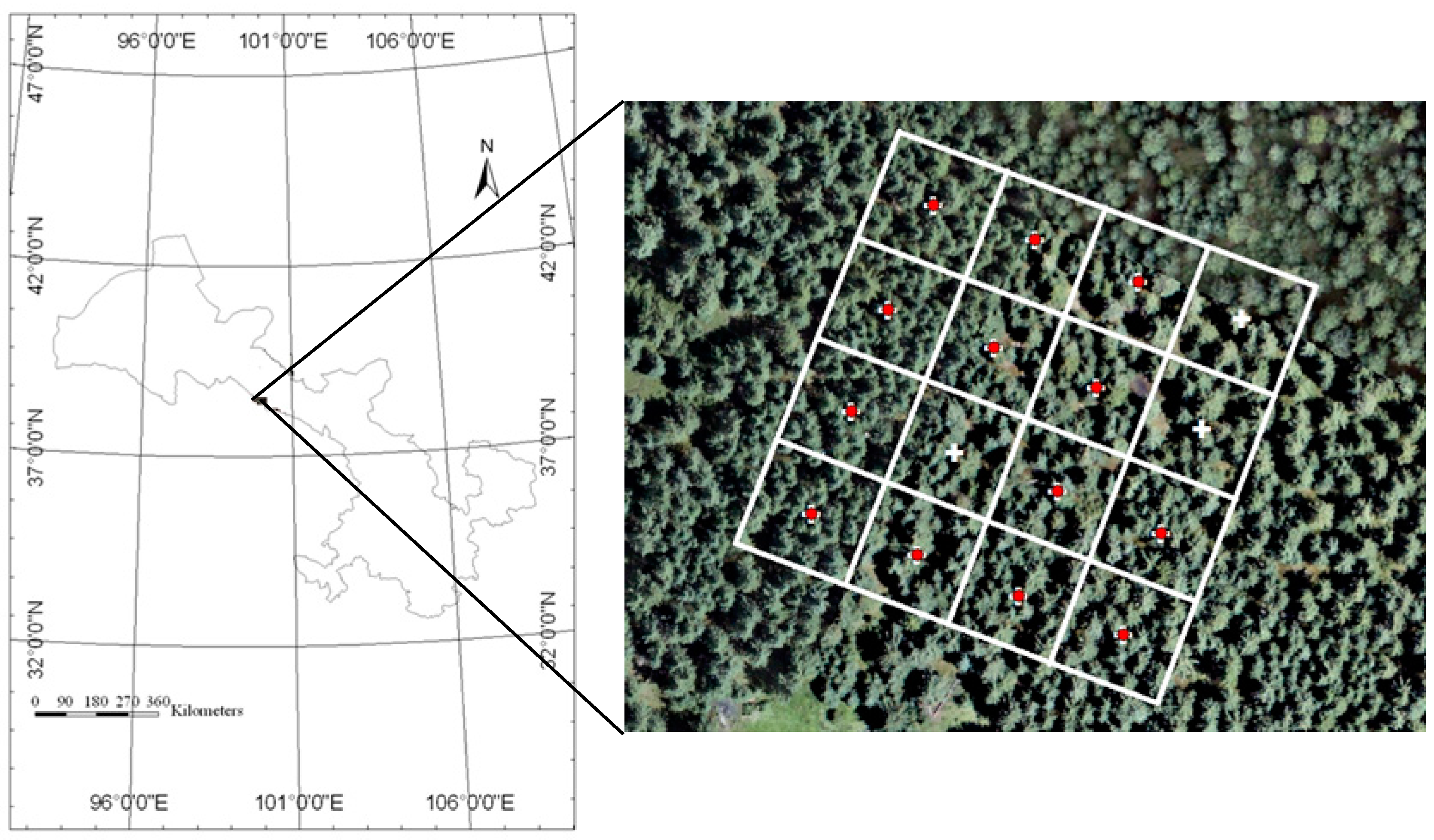
Figure 2.
Intensity of vertical and tilt scanning of the terrestrial laser scanner. (a) Vertical mount; and (b) Tilt mount. The black areas indicate where no points were recorded.
Figure 2.
Intensity of vertical and tilt scanning of the terrestrial laser scanner. (a) Vertical mount; and (b) Tilt mount. The black areas indicate where no points were recorded.
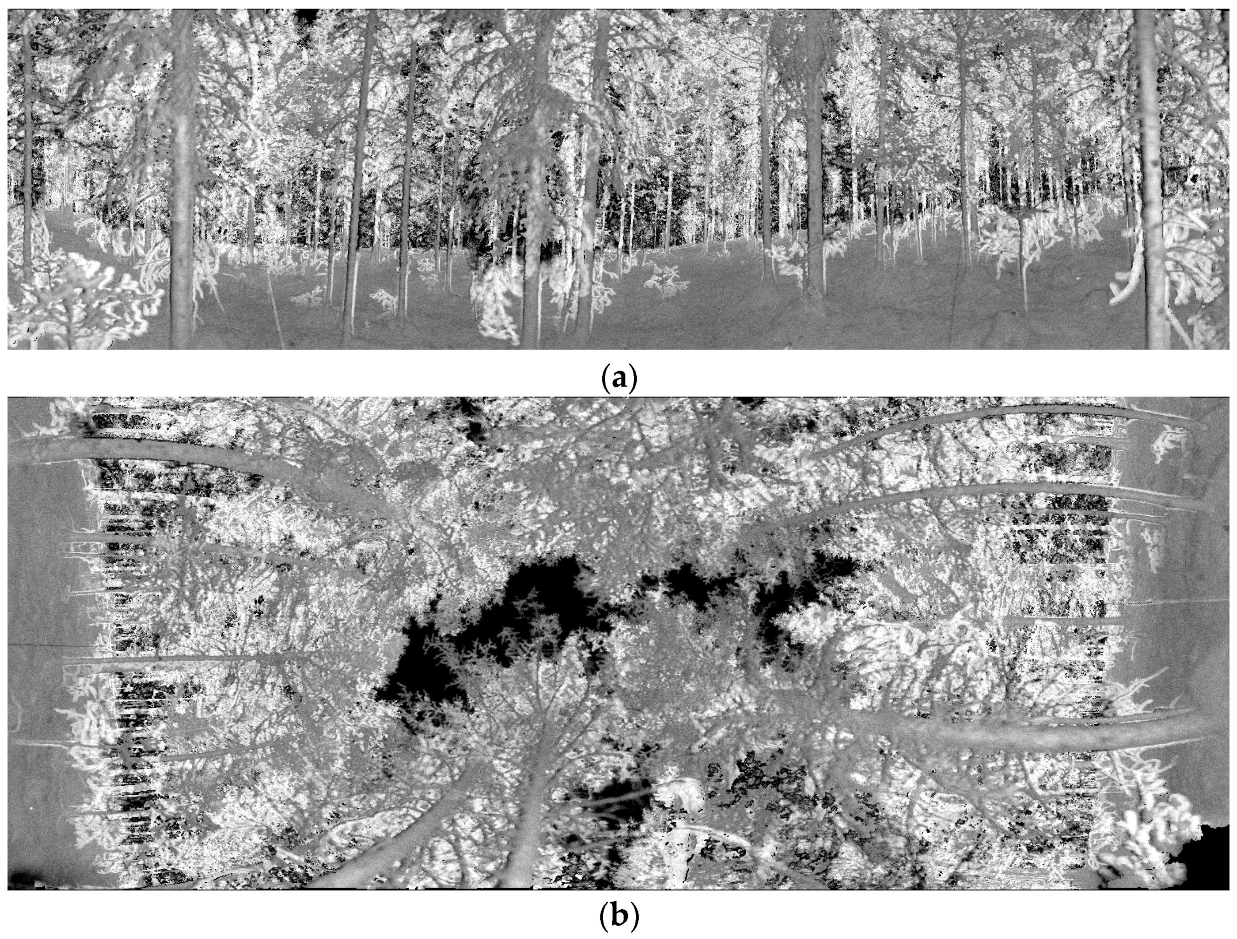
Figure 3.
Example of a hemispherical photograph.
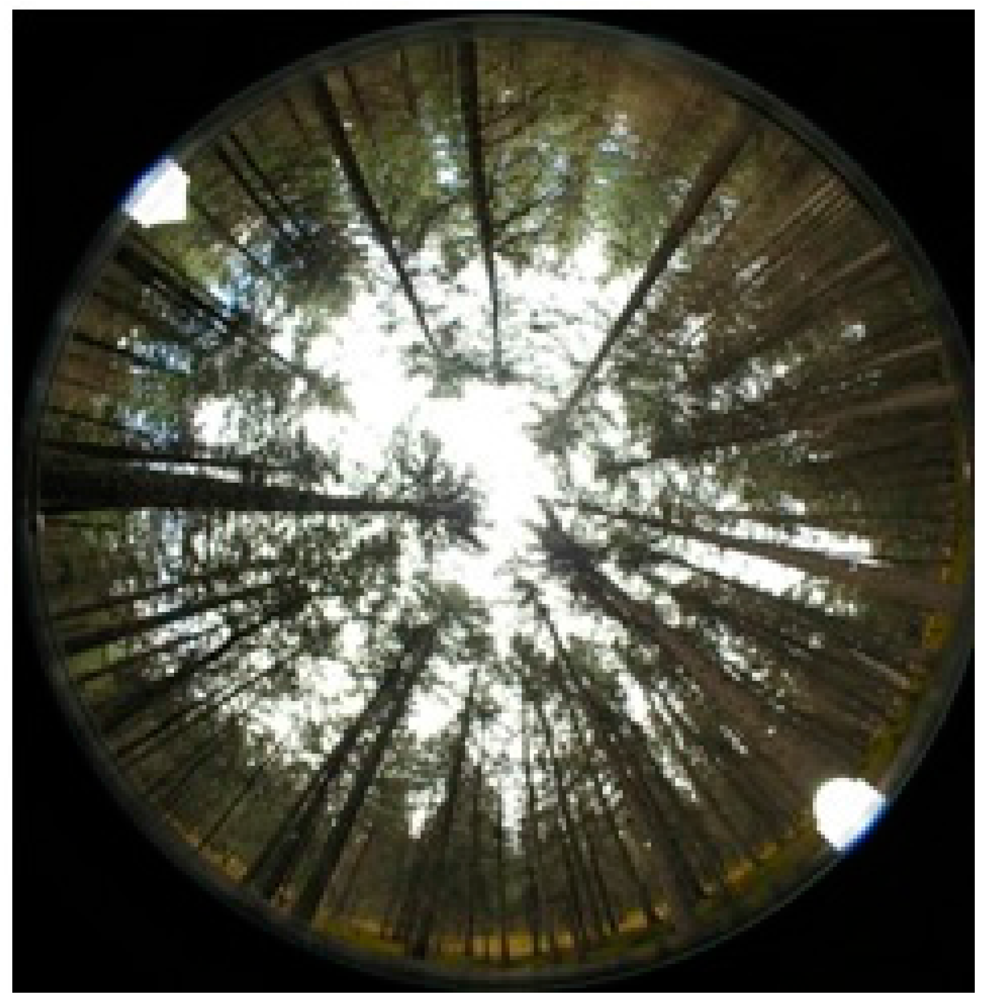
Figure 4.
Sketch of Terrestrial Laser Scanning (TLS) scanning in forests. The center of the circle denotes the position of the laser scan; the green curve denotes the cross section of the trunk surface; and the black zone denotes no point cloud; top view.
Figure 4.
Sketch of Terrestrial Laser Scanning (TLS) scanning in forests. The center of the circle denotes the position of the laser scan; the green curve denotes the cross section of the trunk surface; and the black zone denotes no point cloud; top view.
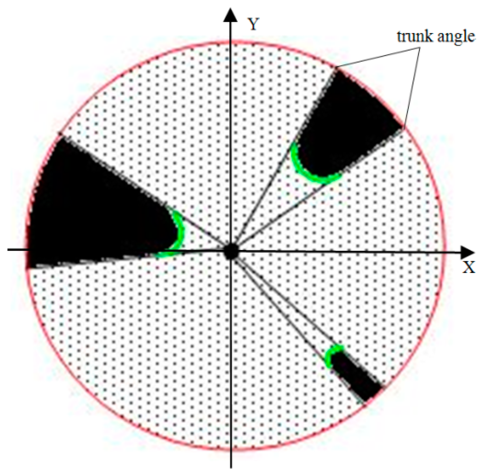
Figure 5.
Angular distribution of the gap fraction distribution. (a) TLS; and (b) HemiView.
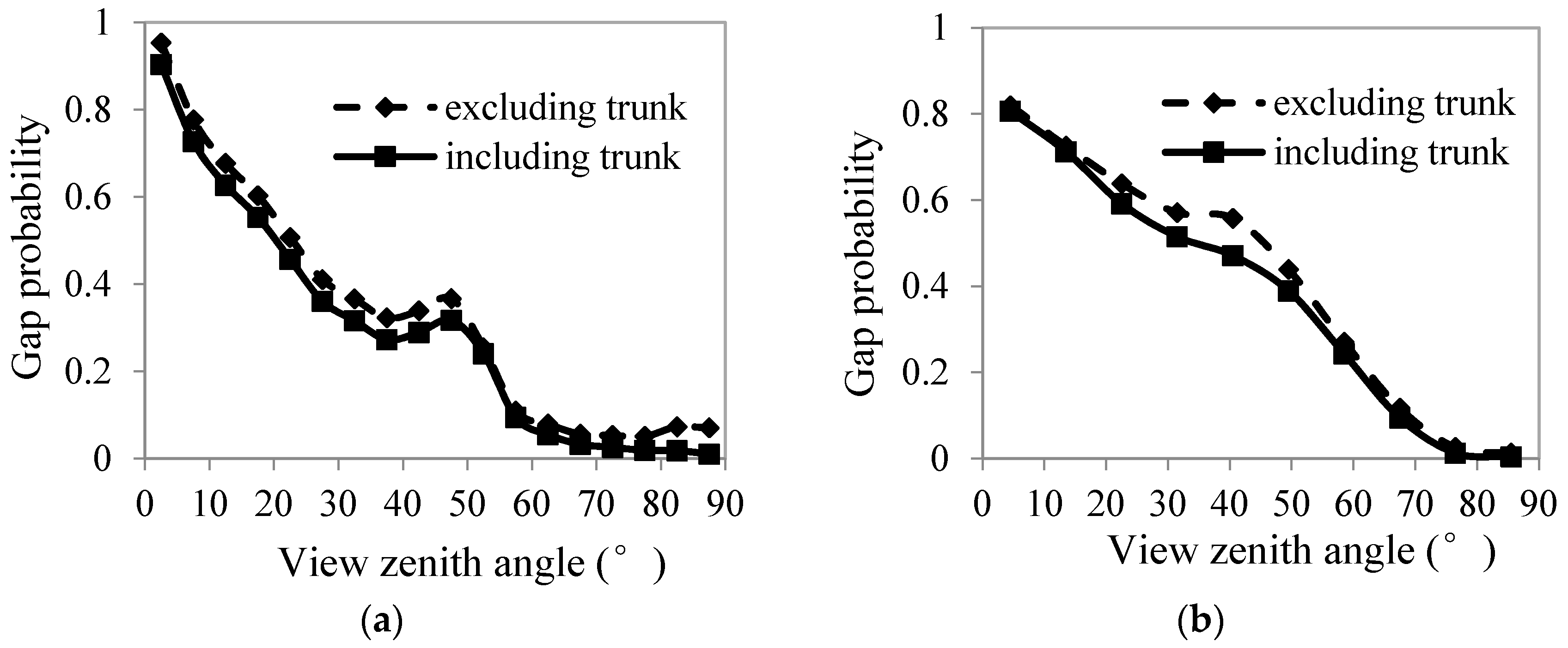
Figure 6.
Angular distribution of the clumping index: (a) TLS; and (b) HemiView.
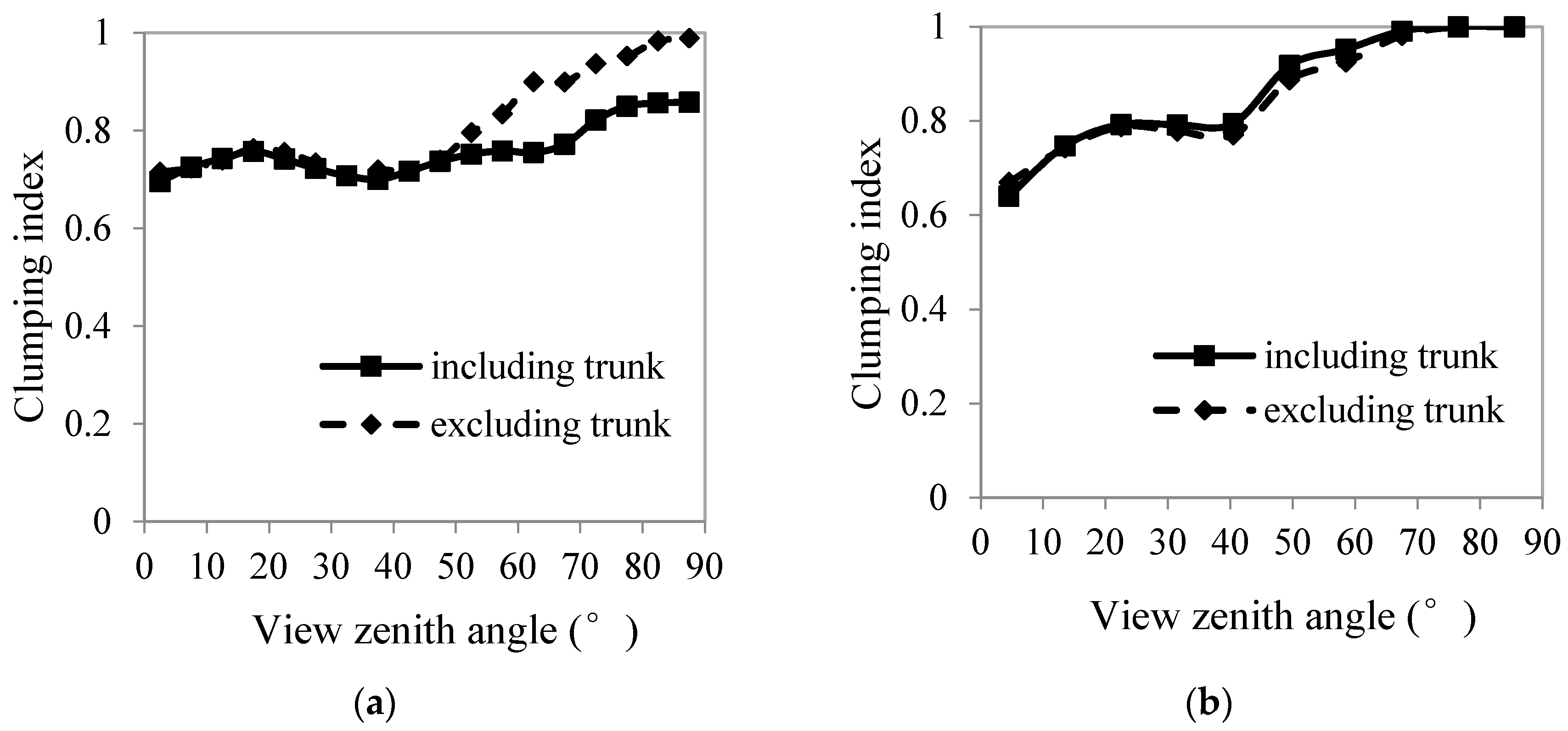
Figure 7.
Comparison of the hemispherical clumping index between TLS and HemiView.
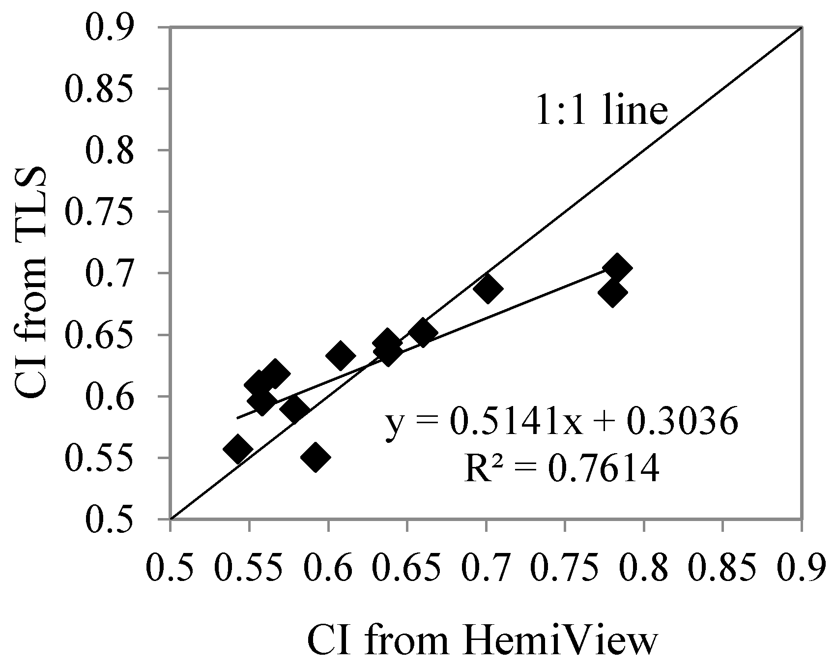
Figure 8.
Angular distribution of Leaf Area Index (LAI). (a) TLS; and (b) HemiView.
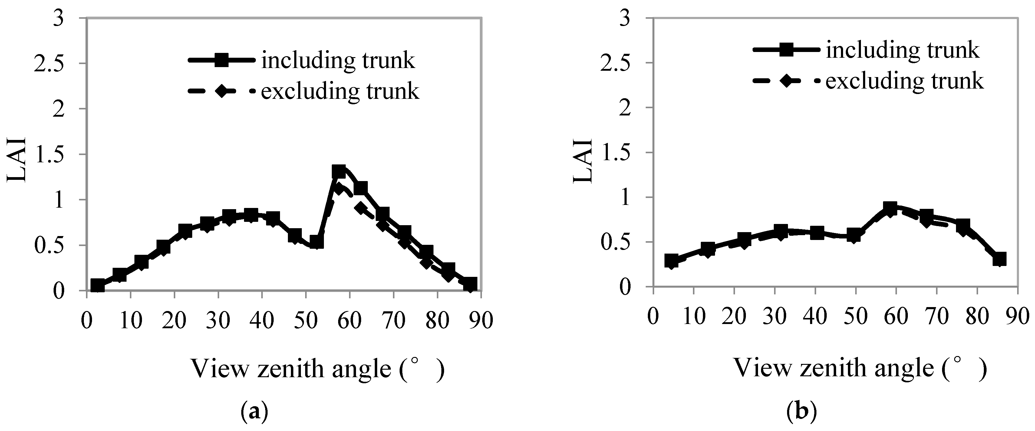
Figure 9.
Comparison of the effective LAI (a), and LAI (b) between TLS and HemiView.
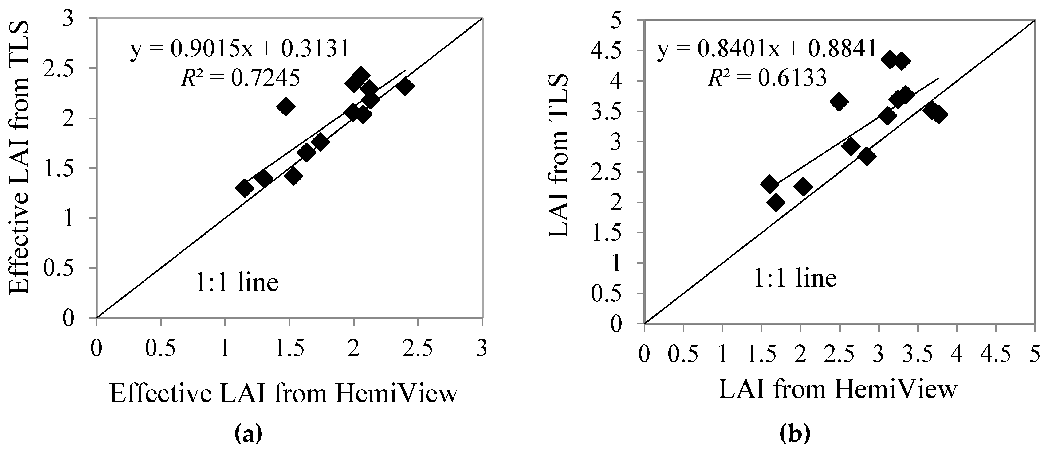
Figure 10.
Comparison of the relative bias (εP, εCI, εL) between TLS and HemiView. (a) Gap probability (P); (b) Clumping index (CI); and (c) LAI (L).
Figure 10.
Comparison of the relative bias (εP, εCI, εL) between TLS and HemiView. (a) Gap probability (P); (b) Clumping index (CI); and (c) LAI (L).

Table 1.
Configuration of the LMS-360i laser scanner.
| Parameters | Characteristics/Value |
|---|---|
| Scanning mechanism | Rotating/oscillating |
| Measurement principle | Single-shot time-of-flight measurement |
| Target detection modes | First, last, or alternating target |
| Laser wavelength | 900 nm |
| Measurement range | 1~200 m |
| Laser pulse repetition rate | 24,000 Hz |
| Laser beam divergence | ≤2 mrad (focused to infinity) |
| Measurement resolution | 5 mm |
| Line scan angle range | −50°~+40° |
| Frame scan angle range | 0°~360° |
| Line angle step width | 0.008° |
| Frame angle step width | 0.01° |
© 2018 by the authors. Licensee MDPI, Basel, Switzerland. This article is an open access article distributed under the terms and conditions of the Creative Commons Attribution (CC BY) license (http://creativecommons.org/licenses/by/4.0/).
Share and Cite
MDPI and ACS Style
Bao, Y.; Ni, W.; Wang, D.; Yue, C.; He, H.; Verbeeck, H. Effects of Tree Trunks on Estimation of Clumping Index and LAI from HemiView and Terrestrial LiDAR. Forests 2018, 9, 144. https://doi.org/10.3390/f9030144
AMA Style
Bao Y, Ni W, Wang D, Yue C, He H, Verbeeck H. Effects of Tree Trunks on Estimation of Clumping Index and LAI from HemiView and Terrestrial LiDAR. Forests. 2018; 9(3):144. https://doi.org/10.3390/f9030144
Chicago/Turabian StyleBao, Yunfei, Wenjian Ni, Dianzhong Wang, Chunyu Yue, Hongyan He, and Hans Verbeeck. 2018. "Effects of Tree Trunks on Estimation of Clumping Index and LAI from HemiView and Terrestrial LiDAR" Forests 9, no. 3: 144. https://doi.org/10.3390/f9030144
Note that from the first issue of 2016, this journal uses article numbers instead of page numbers. See further details here.