Tree- and Stand-Level Biomass Estimation in a Larix decidua Mill. Chronosequence

Abstract

Carbon pool assessments in forests is one of the most important tasks of forest ecology. Despite the wide cultivation range, and economical and traditional importance, the aboveground biomass of European larch (Larix decidua Mill.) stands is poorly characterized. To increase knowledge about forest biomass accumulation and to provide a set of tools for aboveground biomass estimation, we studied a chronosequence of 12 larch forest stands (7–120 years old). From these stands, we measured the biomass of 96 sample trees ranging from 1.9 to 57.9 cm in diameter at breast height. We provided age-specific and generalized allometric equations, biomass conversion and expansion factors (BCEFs) and biomass models based on forest stand characteristics. Aboveground biomass of stands ranged from 4.46 (7-year-old forest stand) to 445.76 Mg ha⁻¹ (106-year-old). Stand biomass increased with increasing stand age, basal area, mean diameter, height and total stem volume and decreased with increasing density. BCEFs of the aboveground biomass and stem were almost constant (mean BCEFs of 0.4688 and 0.3833 Mg m⁻³, respectively). Our generalized models at the tree and stand level had lower bias in predicting the biomass of the forest stands studied, than other published models. The set of tools provided fills the gap in biomass estimation caused by the low number of studies on larch biomass, which allows for better estimation of forest carbon pools.

1. Introduction

In the age of climate change, many ecologists focus their studies on carbon cycling in the biosphere [1,2,3]. Among terrestrial ecosystems, forests are one of the most important carbon reservoirs, accumulating globally ca. 2.4 ± 0.4 × 10¹⁵ g C year⁻¹ [4]. Thus, their role in the mitigating effects of climate change is important [4,5,6]. As climate change will result in changes to tree species’ physiology [7,8] and distributions [8,9,10], adaptation strategies need to be incorporated into forest management. For proper planning of increasing carbon sequestration by forests and calculation of their ability to mitigate climatic change, there is an urgent need to provide accurate carbon assessment tools.

Precise estimation of carbon pools in forest ecosystems are a necessary base for further activities. As carbon content in plant tissues is relatively constant, most inventories focus on biomass estimation [11,12,13,14]. For that reason, accuracy of biomass assessment is crucial for carbon reporting. Different countries use different approaches to country-scale carbon assessment, differing in inventory level (tree or stand level) and accuracy [15]. According to the Intergovernmental Panel on Climate Change (IPCC) guidelines [16], carbon assessment may be based on generalized coefficients. This may lead to underestimation or overestimation of carbon pools in forest stands. For that reason, IPCC recommends usage of locally-fitted models of biomass estimation wherever it is possible.

Forest stand biomass can be estimated at two levels of detail: tree level and stand level. For tree level the most frequent approach is usage of allometric equations (AEs)—regression models allowing for tree biomass estimation using simple measurements, i.e., diameter at breast height or height [17,18,19]. AEs based on individual tree measurements require time- and money-consuming inventories, but yield higher accuracy of biomass estimation. Stand level estimation is usually conducted using forest stand models (e.g., [20,21]) or biomass expansion and conversion factors (BCEFs; e.g., [12,22,23,24]). BCEFs are literally proportions of forest stand biomass and tree stand volume, allowing for easy conversion of forest inventory data (growing stock) into biomass. However, this approach is double-biased by errors of statistical models and errors of forest inventory. For example, BCEFs are not useful in cases of young forest stands where volume of merchantable wood is underestimated [21].

The need for elaboration of more accurate biomass models is connected with the variability of biomass allocation patterns. The proportions of carbohydrates invested in development of particular organs vary climatically [25], but also with increasing age (e.g., [26,27,28]). For that reason, younger trees need separate models both at the tree (e.g., [23,29,30]) and stand (e.g., [21,22,24]) levels. Moreover, according to metabolic scaling theory [31] and its expansion [32], biomass allocation is connected with tree dimensions. In cases of managed forests, initial spacing of forest stands also influence both biomass stock and its allocation [33].

Larix decidua Mill. is a light-demanding, pioneer, coniferous tree species growing naturally in Central Europe across a wide range of altitudes—from 180 (Poland) to 2500 (Alps) m a.s.l. [34]. Since the 16th century L. decidua has been widely cultivated outside its natural range, especially in Great Britain and Scandinavia. According to the FAO Global Forest Resources Assessment [35] country reports, L. decidua growing stock in Europe was 287.9 million m³ in 2010, constituting the seventh largest volume among forestry tree species in Europe. This species is economically and traditionally important due to its fast-growing nature, low soil requirements and high-value wood. Despite its quick biomass increments and wide distribution, little is known about its biomass.

In the database of European allometric equations there were only 11 AEs for L. decidua [19,36]. Forrester et al. [18] found 30 AEs. Our extensive literature review revealed 49 AEs (including those generated by Forrester et al. [18]; Table S1). Except for a dataset of 131 young trees [37], previous studies showed either low numbers of sample trees (up to 45) or limited ranges of diameters. Most of these studies come from the Alps (e.g., [38,39]). Literature review of stand-level biomass estimation for L. decidua also revealed relatively small data sets. Orzeł et al. [40] showed mean BCEF for aboveground biomass of mixed L. decidua forest stands of 0.5828 t m⁻³ and Schepaschenko et al. [41] for Larix spp. stands of 0.640 ± 0.008. BCEFs of Larix sp. as a function of site index, age and relative stocking were provided by Schepaschenko et al. [42] for Russian forests and by Teobaldelli et al. [24] as a function of age and growing stock. However, these studies were general approaches, not fitted specifically to L. decidua as a mountain species. For that reason, there is an urgent need to develop a comprehensive set of allometric equations and BCEFs for L. decidua.

We aimed to provide a comprehensive set of allometric equations (AEs) and biomass conversion and expansion factors (BCEFs) for L. decidua at the tree and stand levels, as well as to assess changes in forest stand biomass and allocation with increasing age and to compare them with published models. We hypothesized that (1) despite poor prediction power of generalized biomass equations, they offer prediction capability for all situations, (2) forest stand features: height, volume, age and density, will influence forest stand biomass and BCEFs and (3) models elaborated using a whole chronosequence will improve biomass estimation accuracy, both at the tree and stand levels, in comparison with previously published approaches.

2. Materials and Methods

2.1. Study Sites and Material

To cover the whole chronosequence of L. decidua forest stands, we chose 12 forest stands in total, one from each 10-year-age class, ranging from 7 to 120 years old (

Table 1. Overview of the study plots and forest stand characteristics.

Latitude (°)	Longitude (°)	Plot Area (ha)	A (year)	V (m3 ha−1)	BA (m2 ha−1)	BA Proportion (%)	N (Ind. ha−1)	DBH (cm)	Hg (m)	AB (Mg ha−1)	BR (Mg ha−1)	FL (Mg ha−1)	ST (Mg ha−1)	BCEFAB	BCEFBR	BCEFFL	BCEFST
51.06401	15.49467	0.0600	7	8.118	1.9	95.0	1650	4.6	4.8	4.64	2.21	0.68	2.09	0.5716	0.2722	0.0838	0.2575
50.86198	18.98410	0.0777	17	219.454	24.8	100.0	1441	14.5	14.9	96.84	14.05	3.40	72.03	0.4413	0.0640	0.0155	0.3282
52.37760	14.93131	0.1200	27	260.712	24.5	99.2	875	18.4	19.5	117.51	10.82	3.29	98.95	0.4507	0.0415	0.0126	0.3795
51.81667	14.77037	0.1950	34	236.789	21.2	98.1	549	22.0	20.6	112.73	11.82	2.12	94.04	0.4761	0.0499	0.0090	0.3971
52.90929	15.37436	0.3364	46	362.072	28.8	99.7	312	33.9	26.0	163.03	17.26	3.61	130.96	0.4503	0.0477	0.0100	0.3617
53.30943	17.25400	0.2750	59	643.078	40.1	91.3	396	35.1	31.6	299.96	21.47	2.87	262.98	0.4664	0.0334	0.0045	0.4089
50.48237	16.80768	0.2016	68	416.150	37.5	84.7 1	526	29.6	23.5	191.45	22.52	1.80	166.30	0.4601	0.0541	0.0043	0.3996
53.13129	19.16529	0.3520	76	421.209	26.9	96.2	307	32.9	31.3	186.96	11.89	2.07	171.72	0.4439	0.0282	0.0049	0.4077
53.90933	14.88185	0.3000	88	615.375	38.4	80.8 2	373	35.6	33.0	280.58	15.37	2.49	259.76	0.4559	0.0250	0.0040	0.4221
54.24200	16.92336	0.5350	96	555.139	34.6	98.6	193	47.4	35.4	257.63	21.17	3.70	231.64	0.4641	0.0381	0.0067	0.4173
54.18082	15.72429	0.3250	106	948.968	51.2	93.3	332	43.8	37.4	445.76	27.27	4.17	406.31	0.4697	0.0287	0.0044	0.4282
49.71889	18.71756	0.6000	120	466.497	28.9	60.7 3	170	45.7	33.9	222.26	19.11	1.76	184.17	0.4764	0.0410	0.0038	0.3948

Abbreviations: A—forest stand age, V—total stem volume, BA—basal area, BA proportion—proportion of L. deciuda basal area in basal area of the whole tree stand, N—forest stand density, DBH—mean diameter at breast height, H_g—mean height weighted by tree basal area, AB—total aboveground biomass, BR—branch biomass, FL—foliage biomass, ST—stem biomass, BCEF_AB—Biomass Conversion and Expansion Factors for total aboveground biomass, BCEF_BR—Biomass Conversion and Expansion Factors for branch biomass, BCEF_FL—Biomass Conversion and Expansion Factors for foliage biomass, BCEF_ST—Biomass Conversion and Expansion Factors for stem biomass. ¹ admixture species: Pinus sylvestris L.—11.8%, other—4.5%; ² admixture species: Picea abies (L.) Karst.—9.7%, other—9.5%; ³ admixture species: Acer pseudoplatanus L.—12.8%, Tilia cordata L.—10.5%, Picea abies—5.9%, Quercus robur L.—5.4%, other—4.7%.

). We searched the Forest Data Bank [43] to find monocultures or forest stands with volume proportion of L. decidua over 70% (within the particular forest compartment). All forest stands grew in managed forests and originated from artificial regeneration. After preselection we consulted local forest inspectorates to exclude stands in which any thinning was performed in the last five years or any damaging agent affected forest stand structure within the last five years. These circumstances allowed for the separating of these potential impacts on biomass crop and allocation. Within each forest stand we established a study plot covering at least 100 trees of L. decidua. Plot size varied from 0.06 to 0.60 ha to maintain the minimal number of measured trees. Sample forest stands grew in mesic or rich forest sites, mostly occupying haplic soils. All plots were located in lowlands and highlands of Western and Southern Poland (49°43′11″–54°14′24″ N; 14°46′12″–19°6′36″ E), in a zone of transition between maritime and continental temperate climate.

2.2. Methods

We conducted our study from July to September 2016 and 2017. Within all study plots we measured diameters at breast height (DBH) of each tree and tree heights (H) of at least 20% of the trees, chosen proportionally to DBH classes. For each plot we determined forest stand density (N), basal area (BA), mean height weighted by tree basal area (H_g), total stem volume (V) and age (A). We used H_g instead of mere mean height, to provide more robust height estimation at the tree stand scale, which is used in biometric studies, e.g., [20,21]. After measurements, we divided trees into nine quantiles and we selected trees at the borders of each quantile as sample trees (8 sample trees per plot) to ensure good representation of all DBH classes. In total, we harvested 96 sample trees, with DBH ranging from 1.9 to 57.9 cm and height from 2.7 to 39.5 m. Each sample tree was cut and divided into stem, merchantable branches (at least 1 m of branch with diameter >7 cm), small branches with foliage and dead branches. We weighed branches with foliage in the field (fresh biomass) and then took samples (at least 5% of their total fresh mass) and divided it into foliage and branches in the laboratory, to assess for dry weight. Sample tree length was measured using a tape after felling. From merchantable branches we took wood and bark samples >0.5 kg. We measured two perpendicular stem diameters for each 1 m length of stem bole (at 0.5 m, 1.5 m and 2.5 m, etc.) to obtain stem volume. Then we divided the stem into three equal-length sections and from the middle of each section we cut a 10–15 cm thick disc. In the field we measured two diameters of discs (maximal and perpendicular to maximal) and thickness in four places (at the points of diameter measurements) to calculate disc volume. We also weighed fresh mass of the discs. In the lab we divided discs into stem wood and stem bark to assess proportion of these components in biomass. This approach is sufficient for proper density estimation, i.e., provides similar accuracy as assessment based on sections cut each 1 m [44]. We also checked that this approach was correct on two of our sample trees, from which we cut discs each 1 m, to ensure that these conclusions [44] may be transferred to L. decidua. We found no difference in density estimation based on discs cut each 1 m and three discs cut at 1/6, 1/2 and 5/6 of stem length

Samples of all material were oven-dried to a constant mass (75 °C) in the laboratory. Then, plant material was weighed with an accuracy of 1 g. Using proportions of dry and fresh masses of samples and total fresh masses of tree components obtained in the field, we calculated total dry mass of each tree component (Table S2). We calculated dry stem mass using proportion between disc and stem section volumes and disc dry mass. As biomass of dead branches and cones strongly varied across study sites and growing seasons, we decided not to analyze them separately, but to incorporate them into aboveground biomass. We prepared a dataset comprised of the following biomass components: SB—stem bark biomass, SW—stem wood biomass, BR—branch biomass, FL—foliage biomass, ST—stem biomass, mABW—merchantable aboveground woody biomass, ABW—aboveground woody biomass, AB—total aboveground biomass. To assess carbon content in stem wood, stem bark, branches and foliage we analyzed three samples of stem wood and bark, and one sample of foliage and branches from each sample tree. This produced 64 samples per study plot (24 of stem wood, 24 of stem bark, 8 of foliage and 8 of branches). We determined carbon content with an ECS CHNS−O 4010 Elemental Combustion System (Costech Instruments, Cernusco sul Naviglio, Italy; Valencia, CA, USA) and CHNS/O Analyser 2400 Series II (Perkin Elmer, Waltham, MA, USA).

2.3. Data Analysis

All analyses were performed using R software [45]. We calculated heights of each tree using the measured heights of 20% of the trees in each forest stand and site-specific Naslund’s models from the lmfor::ImputeHeights() function [46]. For each study plot and biomass component we calculated these ten regression models [21]:

W = a × DBH^b

(1)

W = a + b × DBH²

(2)

W = a + b × log(DBH)

(3)

W = a + (b/DBH)

(4)

W = a × (DBH²H)^b

(5)

W = a × DBH^b × H^c

(6)

W = a + b × log(DBH²H)

(7)

W = a + b × DBH² + c × H

(8)

W = a + b × (DBH²H)

(9)

W = a + b × DBH² + c × H²

(10)

where W—dry mass of the considered biomass component (kg), DBH—diameter at breast height (cm), H—height (m), DBH²H—pseudovolume (m³). Using Akaike’s Information Criterion (AIC) we choose the best fitted model among them. Moreover, we developed a set of generalized equations, using all sample trees. Although study design could influence the model, we decided to use a simpler approach (non-linear models) instead of models with mixed effects (e.g., [47,48]) to increase model applicability.

For comparison of other published models’ transferability to our data, we used observed versus predicted values scatterplots and Nash–Sutcliffe efficiency (NSE):

$$NSE=1-\frac{{{\displaystyle \sum }}_{i=1}^n{\left(y_i-\widehat{y_i}\right)}^2}{{{\displaystyle \sum }}_{i=1}^n{\left(y_i-\overline{y}\right)}^2}$$

(11)

where n—sample size, $y_i$—i-th observed value of y, $\widehat{y_i}$—i-th predicted value of y, $\overline{y}$—mean of y. As reference values (observed) at the tree level we used measured biomass of trees and at the stand level—stand biomass calculated using stand-specific tree-level equations. Although these values are not exact measurements of forest stand biomass, we treated them as the most reliable approximation of stand-level biomass, similarly to other authors, e.g., [12,15,17,21]. For that reason, our study does not compare overall accuracies of the models, but their performance on our dataset. To compare transferability of allometric tree-level models we reviewed published AEs for L. decidua (Table S1). Among 49 AEs found we excluded all equations based on root collar diameter or developed for young forest stands (12 provided by Pajtík et al. [37]), as these stands showed the most different patterns of biomass allocation which did not fulfill the criteria for young forest stands [21]. We also did not compare equations for whole crown biomass provided by Rubatscher et al. [49] as we did not estimate this component separately. We also excluded AEs for belowground parts of trees, as our dataset did not include them. From the study of Usol’tsev et al. [50], who provided two types of models—for six species of Larix pooled together and for L. decidua and L. sukacewii, we chose the latter, as more specific. We also chose the best models given in the cited studies. Therefore, after verification, we used 23 allometric equations for further analyses. To avoid extrapolation bias, we decided to apply the functions to particular trees when the range of dimensions fit into the range from 20% of minimal and 120% of maximal dimension. Thus, only 19 AEs fulfilled these criteria and were compared in terms of differences in biomass predicted by our generalized AEs and published AEs.

For stand-level biomass analyses we calculated biomass conversion and expansion factors (BCEFs) as BCEF = W/V, where W—dry mass of the considered biomass component (Mg ha⁻¹) and V—total stem volume of trees (m³ ha⁻¹). We prepared stand-level estimators for the four most important biomass components—AB, BR, FL and ST. We tried to elaborate multiple regression models for forest stand biomass and BCEFs using forest stand parameters, however, analysis of AIC and variance inflation factors revealed that models with one predictor were the best choice. Variance inflation was high due to intercorrelation of the variables used, as all of them are age-dependent. For that reason we decided to present only these models (Equations (12)–(15)), which allow calculation of forest stand biomass and BCEFs using available variables. For assessment of relationships between BCEFs and forest stand characteristics we used the following model types [21,24,51]:

BCEF = a × z^b

(12)

BCEF = a + b × e^−z×c

(13)

BCEF = a + b/z

(14)

BCEF = a + b/z^c

(15)

where z—forest stand characteristic (forest stand density, height, total stem volume or age), a, b and c—model coefficients and e—base of the natural logarithm. We also used these models (Equations (12)–(15), with W instead of BCEF) to predict relationships between forest stand characteristics and biomass. We chose the best models using AIC. For comparison of model quality, we presented AIC of BCEFs and stand biomass models and AIC₀—AIC of the null model (intercept only).

We compared our stand level AB estimations using both BCEFs and biomass models (based on V and on H_g) with those provided by Teobaldelli et al. [24] and by IPCC. For biomass calculation using BEF (biomass expansion factors, m³ wood of whole tree m⁻³ merchantable wood) we used the following formula:

W = BEF × V_m × ρ

(16)

where BEF—biomass expansion factor, V_m—merchantable volume of the tree and ρ—wood density. As ρ we applied 0.474 Mg m⁻³ [52].

3. Results

3.1. Allometric Equations and Biomass Allocation

Site-specific allometric equations explained from 90.7% to 99.5% of variation in AB biomass, depending on study site (

Table 2. Site-specific equations of biomass components.

Age	Component	Model Type (Equation No.)	a	SE(a)	b	SE (b)	c	SE (c)	RMSE	R2	DBH Range (cm)	Height Range (m)
7	AB	9	0.2690	0.3640	361.2148	47.3346			<0.001	0.907	1.9–5.2	2.7–5.3
7	BR	1	0.0002	0.0005	5.7689	1.4919			0.536	0.868	1.9–5.2	2.7–5.3
7	FL	9	0.0734	0.0436	47.8095	5.6709			<0.001	0.922	1.9–5.2	2.7–5.3
7	ST	9	0.2055	0.0848	149.8650	11.0245			<0.001	0.969	1.9–5.2	2.7–5.3
17	AB	5	173.2234	13.1100	0.8353	0.0788			0.791	0.96	9.5–19.2	13.2–17.2
17	BR	3	−42.5156	5.5634	19.6681	2.1092			<0.001	0.935	9.5–19.2	13.2–17.2
17	FL	5	8.1765	0.5114	1.1229	0.0717			0.013	0.982	9.5–19.2	13.2–17.2
17	ST	5	131.1306	6.7500	0.8520	0.0539			0.205	0.981	9.5–19.2	13.2–17.2
27	AB	5	193.9128	2.7086	1.0372	0.0358			0.885	0.995	11.4–25.6	15.4–22.7
27	BR	1	0.0004	0.0004	3.5199	0.3544			0.578	0.964	11.4–25.6	15.4–22.7
27	FL	2	−1.1134	0.3760	0.0136	0.0009			<0.001	0.972	11.4–25.6	15.4–22.7
27	ST	5	161.9324	4.0845	0.9989	0.0639			0.003	0.983	11.4–25.6	15.4–22.7
34	AB	5	199.8960	2.7170	1.1527	0.0432			0.174	0.993	17.4–27.3	17.9–22.4
34	BR	1	0.0002	0.0002	3.7181	0.3813			0.398	0.943	17.4–27.3	17.9–22.4
34	FL	1	0.0004	0.0007	2.9618	0.5767			0.079	0.81	17.4–27.3	17.9–22.4
34	ST	9	−24.0531	7.8894	192.4834	7.3951			<0.001	0.991	17.4–27.3	17.9–22.4
46	AB	5	179.6590	13.2469	0.9550	0.0547			0.744	0.982	27.1–41.8	24.7–29.7
46	BR	1	0.0034	0.0072	2.7393	0.5869			0.714	0.793	27.1–41.8	24.7–29.7
46	FL	1	0.0004	0.0008	2.8767	0.5191			0.256	0.841	27.1–41.8	24.7–29.7
46	ST	10	−316.3593	91.9174	0.3494	0.0479	0.4878	0.1512	<0.001	0.968	27.1–41.8	24.7–29.7
59	AB	1	0.2435	0.2226	2.2380	0.2470			0.786	0.947	22.9–47.3	28.4–33
59	BR	1	0.0000	0.0000	4.7090	0.4945			1.26	0.964	22.9–47.3	28.4–33
59	FL	10	12.2483	6.7263	0.0082	0.0013	−0.0164	0.0078	<0.001	0.898	22.9–47.3	28.4–33
59	ST	1	0.7330	0.4985	1.8974	0.1847			2.601	0.957	22.9–47.3	28.4–33
68	AB	6	0.0030	0.0041	1.5220	0.1704	2.0752	0.5007	1.655	0.984	20.7–38.9	22.1–28.5
68	BR	6	0.0552	0.2675	3.7571	0.4909	−1.9808	1.5818	0.972	0.938	20.7–38.9	22.1–28.5
68	FL	6	0.0000	0.0000	1.0980	0.6476	3.1397	1.8639	0.034	0.803	20.7–38.9	22.1–28.5
68	ST	6	0.0013	0.0016	1.2980	0.1566	2.5328	0.4565	1.164	0.986	20.7–38.9	22.1–28.5
76	AB	7	−24.4629	56.6312	534.0750	46.7960			<0.001	0.956	24.9–42.3	28.4–33.7
76	BR	5	6.9297	2.0948	1.3505	0.2123			0.055	0.893	24.9–42.3	28.4–33.7
76	FL	6	0.0000	0.0000	1.3738	0.4437	2.7622	1.1472	0.006	0.748	24.9–42.3	28.4–33.7
76	ST	7	−3.8990	49.5803	474.8929	40.9697			<0.001	0.957	24.9–42.3	28.4–33.7
88	AB	7	−290.9563	128.3866	760.0439	88.9083			<0.001	0.924	25.9–47.7	31–35.1
88	BR	7	−44.5787	13.8922	61.8832	9.6204			<0.001	0.873	25.9–47.7	31–35.1
88	FL	7	−4.8755	1.2647	8.3841	0.8758			<0.001	0.939	25.9–47.7	31–35.1
88	ST	7	−227.2036	100.0659	673.1040	69.2961			<0.001	0.94	25.9–47.7	31–35.1
96	AB	8	−2565.2623	737.5435	0.5737	0.0534	73.6682	21.2191	<0.001	0.97	37–55.4	33.8–37.6
96	BR	5	3.3290	2.1150	1.6498	0.2878			0.724	0.87	37–55.4	33.8–37.6
96	FL	5	1.1592	0.8980	1.3332	0.3549			0.017	0.737	37–55.4	33.8–37.6
96	ST	8	−2326.4234	551.2474	0.4812	0.0399	69.0508	15.8594	<0.001	0.977	37–55.4	33.8–37.6
106	AB	5	166.3487	22.0008	1.0427	0.0628			1.477	0.985	31.1–53.1	34.6–39.6
106	BR	6	0.1691	0.4418	4.2628	0.2519	–2.7745	0.6081	1.937	0.99	31.1–53.1	34.6–39.6
106	FL	1	0.0000	0.0000	3.7422	0.6474			0.377	0.89	31.1–53.1	34.6–39.6
106	ST	5	178.1996	26.6103	0.9636	0.0712			1.039	0.977	31.1–53.1	34.6–39.6
120	AB	5	182.4763	39.0245	0.9876	0.0952			6.27	0.958	31.4–57.9	31.1–39.1
120	BR	1	0.0001	0.0001	3.7479	0.6373			3.424	0.903	31.4–57.9	31.1–39.1
120	FL	7	−9.7036	4.0121	10.5079	2.0315			<0.001	0.817	31.4–57.9	31.1–39.1
120	ST	6	0.0017	0.0047	1.5064	0.3351	2.1543	0.9931	4.826	0.957	31.4–57.9	31.1–39.1

Abbreviations: a, b and c—model coefficients, SE—standard error, RMSE—root mean square, AB—total aboveground biomass, BR—branch biomass, FL—foliage biomass, ST—stem biomass; models for other biomass components are given in Table S2.

and Table S3). For BR, FL and ST, coefficients of determination varied from 0.793 to 0.990, from 0.737 to 0.982 and from 0.94 to 0.991, respectively. Generalized allometric equations developed using all sample trees explained from 92.4% to 98.8% of variation in biomass of components studied, with the exception of FL (78.5%,

Table 3. Generalized allometric models for tree biomass for all sample trees (n = 96). For each biomass component we provide the best fit model based on both tree height and diameters at breast height (DBH) as well as on DBH only.

Component	Model Type (Equation No.)	a	SE (a)	b	SE (b)	c	SE (c)	RMSE	R2
AB	6	0.0188	0.0050	1.9093	0.0616	1.0805	0.1077	18.262	0.986
	1	0.1380	0.0315	2.3907	0.0598			27.224	0.971
ABW	6	0.0132	0.0033	1.8721	0.0578	1.2126	0.1019	18.505	0.988
	1	0.1251	0.0297	2.4097	0.0624			30.434	0.969
mABW	10	−123.3840	20.0314	0.4742	0.0244	0.1493	0.0452	<0.001	0.959
	1	0.1015	0.0291	2.4193	0.0752			32.531	0.954
SW	6	0.0069	0.0018	1.7444	0.0574	1.4844	0.1032	13.046	0.988
	1	0.1095	0.0297	2.3986	0.0712			36.316	0.959
SB	6	0.0107	0.0051	1.5474	0.1214	0.9123	0.2057	3.257	0.936
	1	0.0509	0.0162	1.9860	0.0843			5.969	0.922
ST	6	0.0099	0.0025	1.7251	0.0571	1.4266	0.1020	9.739	0.988
	1	0.1397	0.0366	2.3588	0.0689			42.157	0.961
FL	10	1.1890	0.6271	0.0086	0.0008	0.0041	0.0014	<0.001	0.785
	1	0.0046	0.0028	2.1036	0.1606			1.256	0.767
BR	6	0.0091	0.0061	3.7338	0.1886	1.4016	0.2916	8.723	0.924
	1	0.0006	0.0003	3.1484	0.1400			15.034	0.906

Abbreviations: AB—total aboveground biomass, ABW—aboveground woody biomass, mABW—merchantable aboveground woody biomass, SW—stem wood biomass, SB—stem bark biomass, ST—stem biomass, BR—branch biomass, FL—foliage biomass.

). For each component studied, models based on only DBH explained lower amounts of variance and had higher RMSE (root mean square error) than those based on both DBH and height. Stem and total aboveground biomass equations showed better performance than those for branches and foliage (

Table 4. Relationships between forest stand characteristics (predictors) and forest stand biomass components (Mg ha⁻¹).

Component	Predictor	Model No.	a	SE	b	SE	RMSE	R2	AIC	AIC0
AB	age	12	12.2705	11.7614	0.6867	0.2174	6.863	0.664	139.799	150.891
	BA	12	0.75549	0.4965	1.6157	0.1795	1.339	0.922	122.345
	D	12	4.9969	6.3821	1.0788	0.3513	5.553	0.679	139.251
	Hg	12	0.5504	0.7748	1.7781	0.4049	4.901	0.815	132.616
	N	12	3286.8355	4624.5845	−0.4636	0.2424	8.987	0.363	147.474
	V	12	0.3906	0.0341	1.0267	0.0136	0.524	0.999	71.812
BR	age	14	20.4444	1.7098	−134.6048	35.6184	0.000	0.588	73.978	82.624
	BA	12	0.6754	0.4056	0.9368	0.1679	0.203	0.859	61.091
	D	12	1.7065	1.2437	0.6691	0.2040	0.211	0.674	71.176
	Hg	12	1.3204	1.2275	0.7758	0.2738	0.184	0.622	72.947
	N	12	132.6992	128.8053	−0.3462	0.1650	0.220	0.369	79.099
	V	12	0.7273	0.5520	0.5213	0.1213	0.032	0.788	66.028
FL	age	14	3.0803	0.3508	−13.3716	7.3079	0.000	0.251	35.964	37.430
	BA	12	0.6312	0.5232	0.4338	0.2368	0.012	0.434	32.600
	D	14	3.2032	0.3488	−10.7567	4.8131	0.000	0.333	34.568
	Hg	14	3.2938	0.3690	−11.9208	5.1536	0.000	0.349	34.287
	N	12	5.9914	6.2231	−0.1328	0.1717	0.004	0.064	38.632
	V	12	0.5812	0.5185	0.2598	0.1454	0.018	0.390	33.491
ST	age	12	8.8958	9.5380	0.7316	0.2425	7.372	0.652	138.538	149.217
	BA	12	0.4277	0.3140	1.7384	0.1997	0.512	0.915	121.670
	D	12	3.5043	5.0906	1.1418	0.3988	5.955	0.653	138.511
	Hg	12	0.2331	0.3734	1.9904	0.4594	5.456	0.815	130.963
	N	12	3061.5786	4676.0220	−0.4739	0.2634	9.069	0.341	146.204
	V	12	0.2098	0.0299	1.1050	0.0221	0.712	0.997	80.176

Abbreviations: AB—total aboveground biomass, BR—branch biomass, FL—foliage biomass, ST—stem biomass; age—forest stand age (year), BA—basal area (m² ha⁻¹), D—mean diameter (cm), H_g—mean height weighted by tree basal area (m), N—forest stand density (ind. ha⁻¹), V—total stem volume (m³ ha⁻¹), AIC—Akaike’s Information Criterion, AIC₀—AIC of the null model.

). Analysis of residual distributions (Figure 1) showed good fitness for most of the equations. The highest heteroscedasticity was noted for SB, BR and FL models.

Analysis of biomass allocation along a forest stand age gradient (Figure 2) revealed a quick decrease of foliage mass proportion—from 15% in the 7-year-old stand to c.a. 2% in forest stands older than 50 years. Similarly, proportion of branches decreased from 35% to c.a. 5% in older forest stands and proportion of stem increased from 50% in the 7-year-old forest stand to 90% in forest stands older than 60 years.

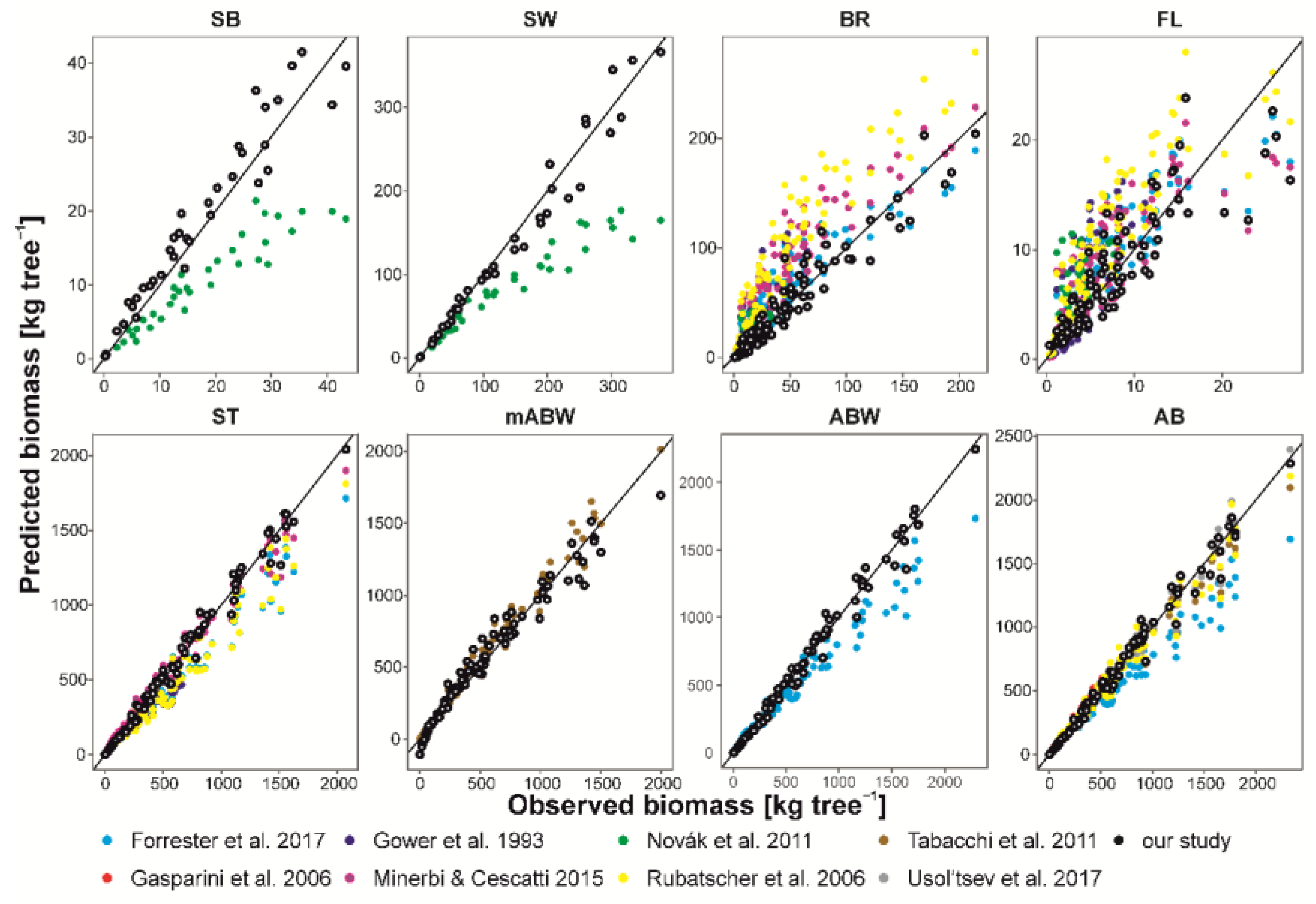
3.2. Comparison of Generalized and Published Allometric Equations Fitness

Our literature review resulted in 19 allometric equations that we were able to compare with our models. Analysis of comparison with original data revealed that some published equations (with the exceptions of FL, BR and mABW AEs) underestimated biomass of our sample trees (Figure 3). Moreover, the trends of equations differed among different authors. In the cases of BR and FL AEs, all estimates showed a wide range of deviations from original data: NSE ranged from −3.28 to 0.82 and from −3.06 to 0.67 for BR and FL, respectively. The lowest difference was found in models provided by Forrester et al. [18]. AEs of Rubatscher et al. [49], Minerbi and Cescatti [39] and Forrester et al. [18] showed overestimation of these biomass components. In the case of mABW we found the highest consistency between our generalized AEs and the model provided by Tabacchi et al. [53], with NSE of 0.97. However, their model slightly underestimated AB (but NSE = 0.97). Models of Gasparini et al. [38] and Usol’tsev et al. [50] were the best predictors of our sample tree AB biomass (NSE of 0.95 and 0.98, respectively), whereas the model proposed by Forrester et al. [18] underestimated AB (NSE = 0.84). Only AB models elaborated by Rubatscher et al. [49] provided a small overestimation (NSE = 0.97). However, this model was the best fit among other published models. Overall, our generalized AEs showed lower deviations from original data and lower heteroscedasticity than published equations (with NSE of 0.98, 0.91, 0.76 and 0.99 for AB, BR, FL and ST, respectively). Analyzing origin of published models, we did not find a geographic pattern in differences of biomass estimates.

3.3. Biomass Accumulation and BCEFs as a Functions of Forest Stand Parameters

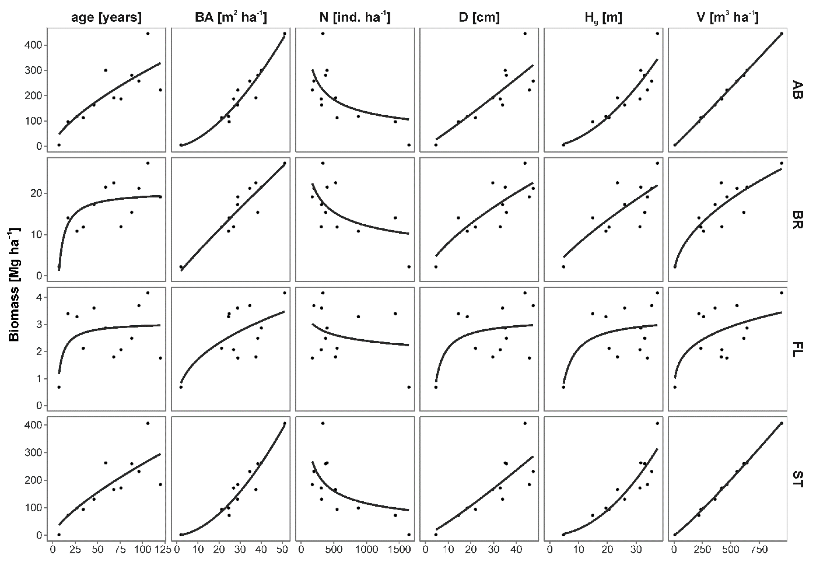
L. decidua forest stand biomass was strongly positively correlated with total stem volume, height and basal area (Figure 4, Table 4). AB and ST had the highest correlations with these predictors and FL had the lowest. The weakest predictor of all analyzed biomass components was forest stand density. Biomass of AB, BR and ST increased with increasing forest stand parameters with the exception of FL. The latter was increasing only between the first two data points (7 and 17 years old forest stands) and then the model curve reached a plateau. The only parameter negatively correlated with biomass was forest stand density.

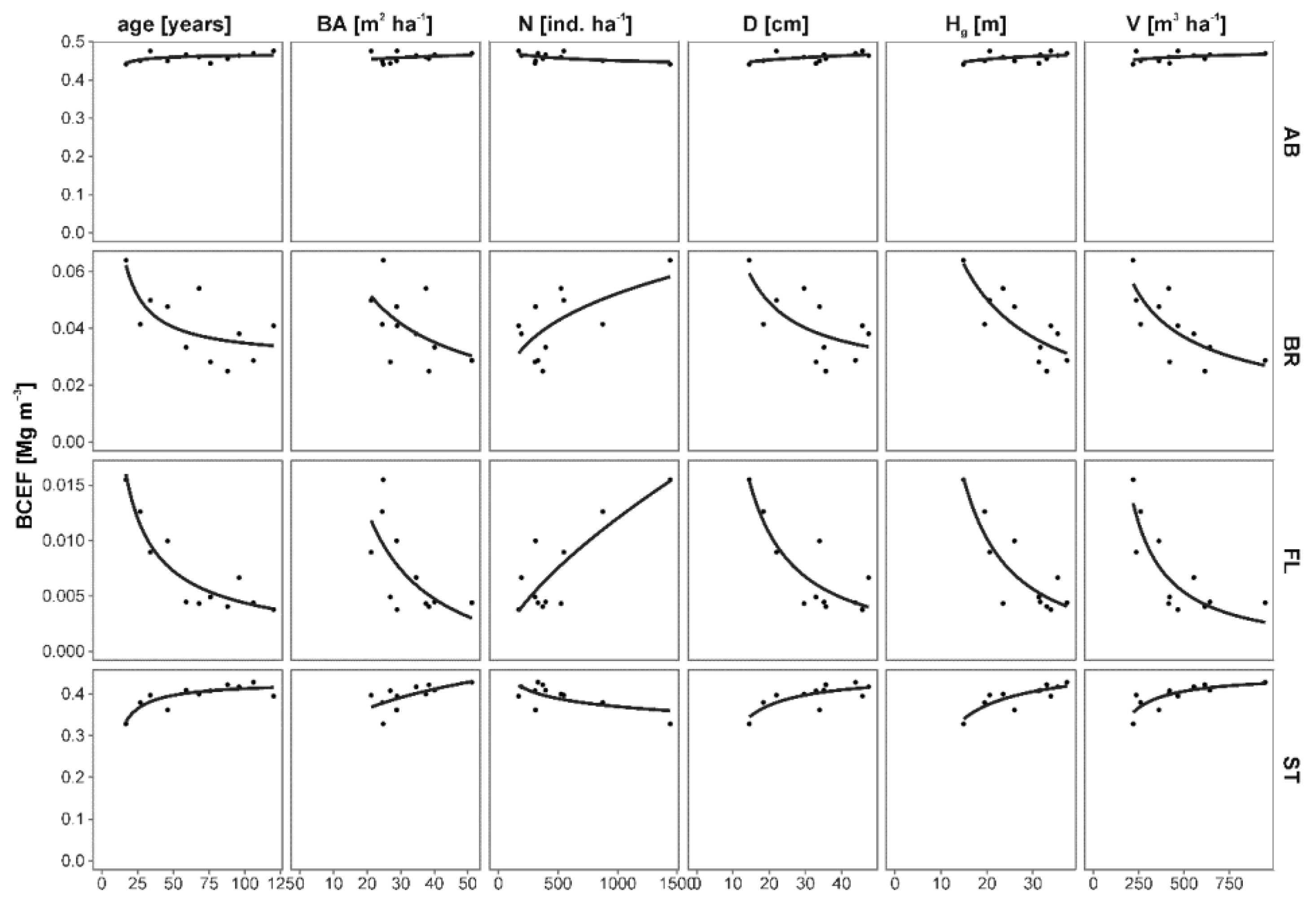
Analysis of BCEF revealed that the young (7 years old) forest stand represented outstandingly higher BCEF than the others (BCEF for AB of 0.5716, BR 0.2722, FL 0.0838), thus all analyses were conducted for 17–120 years old forest stands (Figure S1). The exception was lower BCEF for ST (0.2574). Excluding the 7-year-old forest stand, BCEFs for AB were almost constant with the change of forest stand parameters (Figure 5,

Table 5. Relationships between forest stand characteristics (predictors) and BCEFs for particular biomass components (Mg m⁻³), excluding the youngest stand (7 years old).

Component	Predictor	Model No.	a	SE	b	SE	RMSE	R2	AIC	AIC0
AB	age	14	0.4680	0.0058	−0.4014	0.2273	4.17E−09	0.257	−64.050	−62.778
	BA	12	0.4196	0.0471	0.0264	0.0324	3.23E−07	0.068	−61.550
	D	12	0.4077	0.0284	0.0349	0.0202	6.29E−08	0.251	−63.960
	Hg	14	0.4767	0.0117	−0.4433	0.2877	9.03E−09	0.209	−63.354
	N	12	0.5227	0.0392	−0.0214	0.0124	4.31E−07	0.250	−63.949
	V	12	0.4025	0.0440	0.0219	0.0180	2.05E−07	0.141	−62.446
BR	age	14	0.0292	0.0047	0.5616	0.1827	1.31E−09	0.512	−68.861	−62.962
	BA	12	0.3184	0.3613	−0.5973	0.3353	1.73E−05	0.274	−64.492
	D	14	0.0221	0.0074	0.5410	0.1958	6.59E−09	0.459	−67.719
	Hg	12	0.4885	0.2601	−0.7593	0.1678	4.13E−05	0.677	−73.408
	N	12	0.0070	0.0050	0.2913	0.1139	2.24E−04	0.379	−66.196
	V	12	0.8099	0.6852	−0.4964	0.1437	2.14E−05	0.580	−70.506
FL	age	12	0.1269	0.0394	−0.7311	0.0880	1.40E−05	0.882	−108.868	−87.324
	BA	14	−0.0032	0.0040	0.3189	0.1201	4.16E−09	0.439	−91.685
	D	12	0.3224	0.1977	−1.1375	0.1979	1.40E−04	0.771	−101.543
	Hg	12	0.8084	0.6186	−1.4606	0.2517	4.3132E−05	0.779	−101.913
	N	12	0.0001	0.0001	0.6754	0.1466	2.17E−04	0.665	−97.352
	V	12	5.39667	7.290q	−1.1128	0.2368	2.30E−04	0.738	−100.048
ST	age	14	0.4290	0.0084	−1.6177	0.3281	7.80E−09	0.730	−55.973	−43.580
	BA	12	0.2156	0.0542	0.1753	0.0723	9.40E−06	0.391	−47.030
	D	14	0.4471	0.0154	−1.4884	0.4081	3.57E−08	0.596	−51.563
	Hg	14	0.4707	0.0170	−1.9517	0.4192	1.85E−08	0.707	−55.068
	N	12	0.6135	0.1170	−0.0733	0.0318	5.78E−05	0.387	−46.959
	V	14	0.4461	0.0146	−19.8373	5.1984	2.64E−07	0.618	−52.167

Abbreviations: AB—total aboveground biomass, BR—branch biomass, FL—foliage biomass, ST—stem biomass; age—forest stand age (years), BA—basal area (m² ha⁻¹), D—mean diameter (cm), H_g—mean height weighted by tree basal area (m), N—forest stand density (ind. ha⁻¹), V—total stem volume (m³ ha⁻¹).

). BCEFs for ST were slightly increasing and for BR and FL were significantly decreasing with increasing forest stand age and dimensions. The best predictors (except for total stem volume) of BCEFs were forest stand age and height, and the worst were basal area and density.

3.4. Comparison of Stand Level Biomass Models

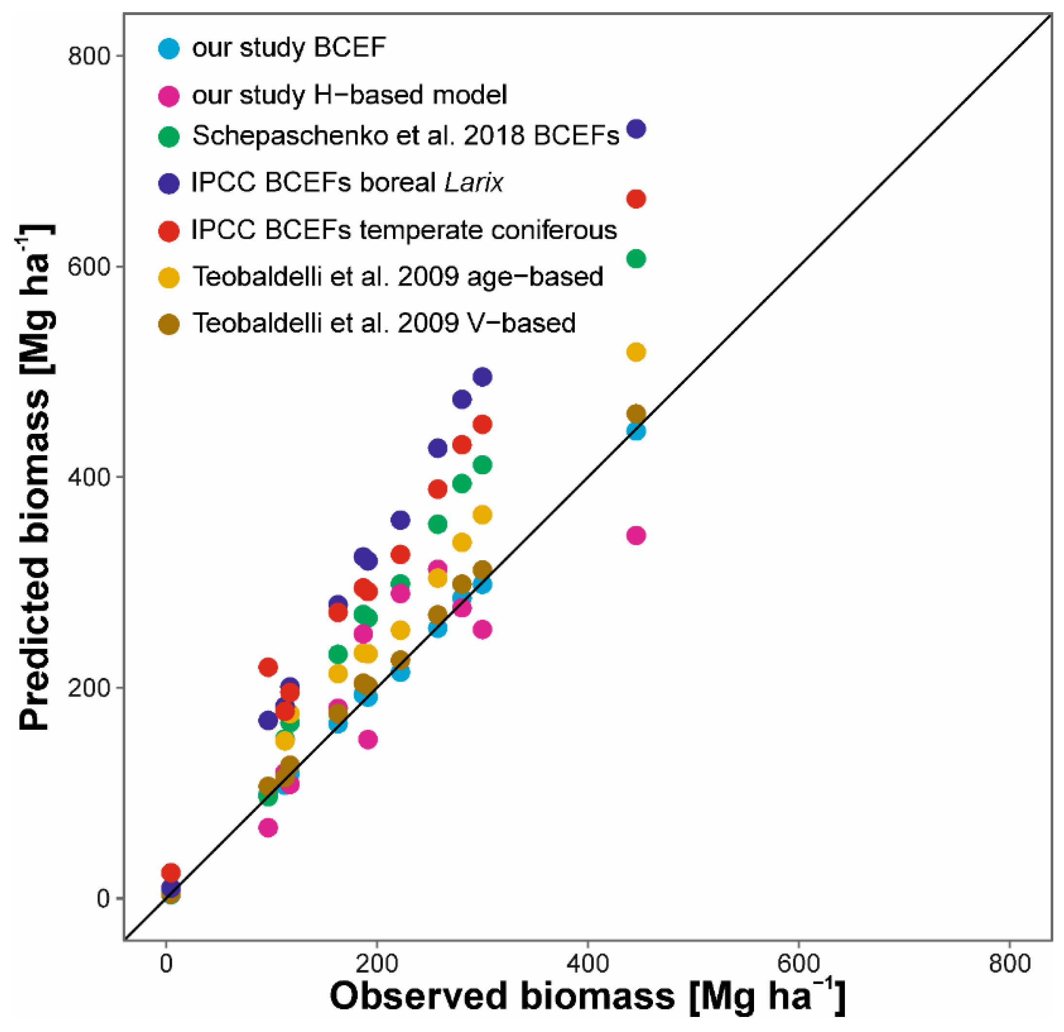
Analysis of accuracy of our and published models for biomass estimation at the stand level revealed that height-based models and estimation using BCEF models provided the lowest biases (Figure 6, NSE of 0.81 and 0.99, respectively). Approaches recommended by IPCC and Schepaschenko et al. [41] provided overestimated biomass, which deviated the most in cases of the biggest forest stands (NSE of −0.86, −0.23 and 0.40, respectively). Models provided by Teobaldelli et al. [24] provided lower overestimation of L. decidua biomass (NSE of 0.77 and 0.99, for age- and volume-based models, respectively). Our model based on forest stand heights underestimated biomass in almost all cases. We found the lowest deviations from observed values for our BCEF model and growing stock volume-based models of Teobaldelli et al. [24].

3.5. Carbon Content

Carbon content in samples differed across tree components and forest stand age (

Table 6. Relationships between forest stand age and carbon content (%) assessed using linear regression.

Component	Term	Estimate	SE	t	Pr (>|t|)
stem wood	(Intercept)	49.488	0.074	666.145	<0.001
R2 = 0.001	age	0.004	0.001	3.831	<0.001
stem bark	(Intercept)	51.762	0.186	279.037	<0.001
R2 = 0.001	age	0.003	0.003	1.058	0.291
branches	(Intercept)	51.123	0.178	287.988	<0.001
R2 = 0.011	age	0.004	0.003	1.340	0.185
foliage	(Intercept)	49.374	0.246	201.083	<0.001
R2 = 0.031	age	0.007	0.003	2.013	0.047

). However, the rate of carbon content increase was low (but statistically significant for all components with the exceptions of bark and fine branches)—from 0.003% (bark) to 0.007% (foliage) per year within the chronosequence studied. Mean carbon content was 49.435 ± 0.037% in stem wood, 51.933 ± 0.091% in stem bark, 51.332 ± 0.084% in fine branches and 49.805 ± 0.123% in foliage. Carbon content for whole tree weighted by share of biomass component ranged from 49.48% (76-year-old forest stand) to 50.74% (106-year-old forest stand), with an average of 50.134 ± 0.099%.

4. Discussion

4.1. Accuracy of the Tree-Level Models

Our generalized tree-level models showed good performance for most of the biomass components studied. Their quality was comparable to generalized equations provided by Muukkonen [54]. However, comparison of our models with generalized equations elaborated by Forrester et al. [18] revealed that the latter models underestimated AB, ST and (slightly) ABW. This may result from combining allometric equations with different quality. A Czech study of young forest stands [55] showed high deviation from our models for SB and SW. In the cited study stem biomass was estimated using narrow discs (2 cm), which could also affect the biomass assessment. Another explanation is narrower range of sample tree diameters, which resulted in different biomass allocation patterns [29,56,57]. This may be especially significant in for overestimation of BR and FL by AEs derived in the Alps [39,49,53]. We found similar deviations between specific results for a ST model from an experimental site in the USA [58]. We found the highest consistency with observed biomass in models from Italy [53] and all of Eurasia [50]. The highest variability and the lowest coefficients of determination were found for models of foliage and branch biomass. We observed this trend both in our models, in L. decidua models provided by other studies, as well as in other species [19,21,36].

Our study also revealed carbon content lower than 51%—a value provided by IPCC guidelines [16]. Although our results were within the uncertainty range provided by IPCC (from 47% to 55%), using the proposed mean value (51%) we overestimated carbon content in stem wood, which is a main component of forest stand biomass. For example, in a 68-year-old forest stand, 1% overestimation of carbon content is equal to 1.66 Mg C ha⁻¹ and in a 106-year-old stand, is equal to 4.06 Mg C ha⁻¹.

4.2. Accuracy of Stand-Level Biomass Models

Our study provided a comprehensive set of tools for tree- and stand-level biomass estimation of L. decidua. Although previous AEs allowed for reliable estimates, the new models increased their accuracy. However, the most important improvement occurred at the stand level. Previous approaches provided by IPCC [16] and Teobaldelli et al. [24] resulted in overestimation of biomass. Models provided by Teobaldelli et al. [24] overestimated, on average, 18.0% and 32.3% for V-based and age-based BEF models, respectively. Applying BCEF values for boreal Larix from IPCC guidelines resulted in an average of 71.5% higher biomass and for temperate coniferous excluding Pinus—an average of 91.8% higher biomass. Some studies provide BCEF values lower than those provided by IPCC [21,41]. However, applying the lower value of the range provided by IPCC to temperate coniferous species resulted in mean underestimation of biomass by an average of 19.9%. This wide range of uncertainty highlights the need for providing locally-fit models. This tendency was also reflected in the study of Schepaschenko et al. [41], who found high-level geographic variability of BCEFs values across climatic gradients in Russia. The high variability of BCEFs provided by IPCC is most probably connected with its wide range of geographic origin: among eight source studies one comes from China, one form Japan, one from Australia, four from USA and one from Germany. For that reason, IPCC BCEFs do not have good fits for European forests. The differences may also result from different methods of forest stand volume estimation in previous studies, e.g., based on forest stand volume tables.

4.3. Influence of Forest Stand Parameters on Biomass Estimation

Analyses of biomass changes along increasing forest stand parameters revealed quick biomass increments of BR and FL in the youngest forest stands. Increments of AB and ST were not so dynamic in the first twenty years. In the case of BCEFs the youngest forest stand in our dataset was an outlier. This is connected with quick decreases of leaf and branch proportions in biomass in the first ten years of tree growth [13,57,59]. Similar results were reported for Pinus sylvestris L. [21] and Betula pendula Roth. [22], as well as for chronosequences of other species, regardless of pooling them together or treating them separately [24,60]. For that reason, BR and FL models were more biased than ST and AB, at both the tree and stand levels. However, excluding the youngest plots, models providing biomass estimation based on forest stand features had good quality. Biomass was mostly correlated with forest stand dimensions. In almost all cases age and density (parameters not strictly correlated with dimensions) were the worst predictors of biomass. BCEFs for AB and its main component—ST—were almost constant across forest stand characteristics, excluding the youngest forest stand. This trend was also reported by other studies (e.g., [24,60,61]). The most likely reason is that when stem mass fraction increases with increasing tree dimensions, it becomes the main component of the tree, and BCEF value tends to wood density.

In contrast to other forest stand parameters, forest stand density was negatively correlated with BCEFs and biomass. During growth of forest stands, initial densities decrease due to management thinning and self-thinning processes. These changes which accompany stand development influence tree diameters at breast height, tree heights, diameters and lengths of tree crowns, and diameters and lengths of branches, thus they influence vertical and horizontal stand structure. Silviculture at variable stand densities may also lead to changes in biomass allocation to aboveground and belowground parts of trees and these changes may by influenced by light demands of particular tree species. Although initial forest stand density affects forest stand productivity and biomass allocation of P. sylvestris forest stands [33,62], we did not find this pattern in the studied L. decidua forest stands. Castedo-Dorado et al. [20] presented stand-level biomass estimation for six tree species (including three conifers: Pinus pinaster Aiton, P. radiata D. Don and P. sylvestris), and found that forest stand density was the weakest predictor of forest stand biomass. It may be connected with the trade-off in usage of resources between trees in dense and sparse forest stands—the same amount of light allows for growth of more trees with thinner trunks or fewer with thicker trunks, and also influences belowground biomass [41]. Thus, it is also possible that trees growing in lower density stands invest more resources to belowground biomass (e.g., to coarse roots) for mechanical stability than to aboveground biomass for better capture of light. Moreover, on soils with similar growth potential (available resources), total aboveground biomass of trees may be lower in more sparse stands than in dense stands, however biomass partitioning in the aboveground parts of trees may be similar.

5. Conclusions

Our study provided a comprehensive overview of the tree- and stand-level assessments of aboveground biomass estimation for L. decidua. We updated the state of knowledge about biomass accumulation and carbon sequestration by this important tree species. We also showed that most of the previous studies underestimated the biomass of L. decidua. Our models performed better than other European AEs and stand-level estimation methods. The set of tools provided by our study fills the gap in biomass estimation caused by the low number of studies on L. decidua biomass, which allows better estimation of forest carbon pools. For stand-level estimations we recommend usage of volume-based models; however, if the stand volume is not known, the biomass may be estimated using height-based models. At the tree level we recommend usage of our site-specific models, but only when range of trees dimensions is similar to range of sample trees used for developing the particular model. Otherwise usage of generalized equations would provide more robust estimations.

References

- Intergovernmental Panel on Climate Change. Climate Change 2013: The Physical Science Basis. Contribution of Working Group I to the Fifth Assessment Report of the Intergovernmental Panel on Climate Change; Cambridge University Press: Cambridge, UK; New York, NY, USA, 2013. [Google Scholar]
- Sohngen, B.; Tian, X. Global climate change impacts on forests and markets. For. Policy Econ. 2016, 72, 18–26. [Google Scholar] [CrossRef]
- Thuiller, W.; Lavergne, S.; Roquet, C.; Boulangeat, I.; Lafourcade, B.; Araujo, M.B. Consequences of climate change on the tree of life in Europe. Nature 2011, 470, 531–534. [Google Scholar] [CrossRef] [PubMed]
- Pan, Y.; Birdsey, R.A.; Fang, J.; Houghton, R.; Kauppi, P.E.; Kurz, W.A.; Phillips, O.L.; Shvidenko, A.; Lewis, S.L.; Canadell, J.G.; et al. A Large and Persistent Carbon Sink in the World’s Forests. Science 2011, 333, 988–993. [Google Scholar] [CrossRef] [PubMed]
- Naudts, K.; Chen, Y.; McGrath, M.J.; Ryder, J.; Valade, A.; Otto, J.; Luyssaert, S. Europe’s forest management did not mitigate climate warming. Science 2016, 351, 597–600. [Google Scholar] [CrossRef] [PubMed]
- Seidl, R.; Schelhaas, M.-J.; Rammer, W.; Verkerk, P.J. Increasing forest disturbances in Europe and their impact on carbon storage. Nat. Clim. Chang. 2014, 4, 806–810. [Google Scholar] [CrossRef] [PubMed] [Green Version]
- Chmura, D.J.; Howe, G.T.; Anderson, P.D.; St. Clair, B. Adaptation of trees, forests and forestry to climate change. Sylwan 2010, 154, 587–602. [Google Scholar]
- Lindner, M.; Fitzgerald, J.B.; Zimmermann, N.E.; Reyer, C.; Delzon, S.; van der Maaten, E.; Schelhaas, M.-J.; Lasch, P.; Eggers, J.; van der Maaten-Theunissen, M.; et al. Climate change and European forests: What do we know, what are the uncertainties, and what are the implications for forest management? J. Environ. Manag. 2014, 146, 69–83. [Google Scholar] [CrossRef] [PubMed]
- Dyderski, M.K.; Paź, S.; Frelich, L.E.; Jagodziński, A.M. How much does climate change threaten European forest tree species distributions? Glob. Chang. Biol. 2018, 24, 1150–1163. [Google Scholar] [CrossRef] [PubMed]
- Meier, E.S.; Lischke, H.; Schmatz, D.R.; Zimmermann, N.E. Climate, competition and connectivity affect future migration and ranges of European trees. Glob. Ecol. Biogeogr. 2012, 21, 164–178. [Google Scholar] [CrossRef]
- Jagodziński, A.M.; Jarosiewicz, G.; Karolewski, P.; Oleksyn, J. Carbon concentration in the biomass of common species of understory shrubs. Sylwan 2012, 156, 650–662. [Google Scholar]
- Lehtonen, A.; Mäkipää, R.; Heikkinen, J.; Sievänen, R.; Liski, J. Biomass expansion factors (BEFs) for Scots pine, Norway spruce and birch according to stand age for boreal forests. For. Ecol. Manag. 2004, 188, 211–224. [Google Scholar] [CrossRef] [Green Version]
- Uri, V.; Varik, M.; Aosaar, J.; Kanal, A.; Kukumägi, M.; Lõhmus, K. Biomass production and carbon sequestration in a fertile silver birch (Betula pendula Roth) forest chronosequence. For. Ecol. Manag. 2012, 267, 117–126. [Google Scholar] [CrossRef]
- Xie, X.; Cui, J.; Shi, W.; Liu, X.; Tao, X.; Wang, Q.; Xu, X. Biomass partition and carbon storage of Cunninghamia lanceolata chronosequence plantations in Dabie Mountains in East China. Dendrobiology 2016, 76, 165–174. [Google Scholar] [CrossRef]
- Neumann, M.; Moreno, A.; Mues, V.; Härkönen, S.; Mura, M.; Bouriaud, O.; Lang, M.; Achten, W.M.J.; Thivolle-Cazat, A.; Bronisz, K.; et al. Comparison of carbon estimation methods for European forests. For. Ecol. Manag. 2016, 361, 397–420. [Google Scholar] [CrossRef]
- Eggleston, S.; Buedia, L.; Miwa, K.; Ngara, T.; Tanabe, K. 2006 IPCC Guidelines for National Greenhouse Gas Inventories; Institute for Global Environmental Strategie: Hayama, Japan, 2006. [Google Scholar]
- Baskerville, G.L. Use of Logarithmic Regression in the Estimation of Plant Biomass. Can. J. For. Res. 1972, 2, 49–53. [Google Scholar] [CrossRef]
- Forrester, D.I.; Tachauer, I.H.H.; Annighoefer, P.; Barbeito, I.; Pretzsch, H.; Ruiz-Peinado, R.; Stark, H.; Vacchiano, G.; Zlatanov, T.; Chakraborty, T.; et al. Generalized biomass and leaf area allometric equations for European tree species incorporating stand structure, tree age and climate. For. Ecol. Manag. 2017, 396, 160–175. [Google Scholar] [CrossRef]
- Zianis, D.; Muukkonen, P.; Mäkipää, R.; Mencuccini, M. Biomass and stem volume equations for tree species in Europe; Silva Fennica Monographs: Helsinki, Finnland, 2005. [Google Scholar]
- Castedo-Dorado, F.; Gómez-García, E.; Diéguez-Aranda, U.; Barrio-Anta, M.; Crecente-Campo, F. Aboveground stand-level biomass estimation: A comparison of two methods for major forest species in northwest Spain. Ann. For. Sci. 2012, 69, 735–746. [Google Scholar] [CrossRef]
- Jagodziński, A.M.; Dyderski, M.K.; Gęsikiewicz, K.; Horodecki, P.; Cysewska, A.; Wierczyńska, S.; Maciejczyk, K. How do tree stand parameters affect young Scots pine biomass?—Allometric equations and biomass conversion and expansion factors. For. Ecol. Manag. 2018, 409, 74–83. [Google Scholar] [CrossRef]
- Jagodziński, A.M.; Zasada, M.; Bronisz, K.; Bronisz, A.; Bijak, S. Biomass conversion and expansion factors for a chronosequence of young naturally regenerated silver birch (Betula pendula Roth) stands growing on post-agricultural sites. For. Ecol. Manag. 2017, 384, 208–220. [Google Scholar] [CrossRef]
- Pajtík, J.; Konôpka, B.; Lukac, M. Biomass functions and expansion factors in young Norway spruce (Picea abies [L.] Karst) trees. For. Ecol. Manag. 2008, 256, 1096–1103. [Google Scholar] [CrossRef]
- Teobaldelli, M.; Somogyi, Z.; Migliavacca, M.; Usoltsev, V.A. Generalized functions of biomass expansion factors for conifers and broadleaved by stand age, growing stock and site index. For. Ecol. Manag. 2009, 257, 1004–1013. [Google Scholar] [CrossRef]
- Oleksyn, J.; Reich, P.B.; Chalupka, W.; Tjoelker, M.G. Differential Above- and Below-ground Biomass Accumulation of European Pinus sylvestris Populations in a 12-year-old Provenance Experiment. Scand. J. For. Res. 1999, 14, 7–17. [Google Scholar] [CrossRef]
- Blujdea, V.N.B.; Pilli, R.; Dutca, I.; Ciuvat, L.; Abrudan, I.V. Allometric biomass equations for young broadleaved trees in plantations in Romania. For. Ecol. Manag. 2012, 264, 172–184. [Google Scholar] [CrossRef]
- Donnelly, L.; Jagodziński, A.M.; Grant, O.M.; O’Reilly, C. Above- and below-ground biomass partitioning and fine root morphology in juvenile Sitka spruce clones in monoclonal and polyclonal mixtures. For. Ecol. Manag. 2016, 373, 17–25. [Google Scholar] [CrossRef] [Green Version]
- Peichl, M.; Arain, M.A. Allometry and partitioning of above- and belowground tree biomass in an age-sequence of white pine forests. For. Ecol. Manag. 2007, 253, 68–80. [Google Scholar] [CrossRef]
- Jagodziński, A.M.; Kałucka, I.; Horodecki, P.; Oleksyn, J. Aboveground biomass allocation and accumulation in a chronosequence of young Pinus sylvestris stands growing on a lignite mine spoil heap. Dendrobiology 2014, 72, 139–150. [Google Scholar] [CrossRef]
- Pajtík, J.; Konôpka, B.; Seben, V. Mathematical Biomass Models for Young Individuals of Forest Tree Species in the Region of the Western Carpathians; National Forest Centre: Zvolen, Slovakia, 2018. [Google Scholar]
- Enquist, B.J.; Niklas, K.J. Global allocation rules for patterns of biomass partitioning in seed plants. Science 2002, 295, 1517–1520. [Google Scholar] [CrossRef] [PubMed]
- Poorter, H.; Jagodzinski, A.M.; Ruiz-Peinado, R.; Kuyah, S.; Luo, Y.; Oleksyn, J.; Usoltsev, V.A.; Buckley, T.N.; Reich, P.B.; Sack, L. How does biomass distribution change with size and differ among species? An analysis for 1200 plant species from five continents. New Phytol. 2015, 208, 736–749. [Google Scholar] [CrossRef] [PubMed] [Green Version]
- Jagodziński, A.M.; Oleksyn, J. Ecological consequences of silviculture at variable stand densities. II. Biomass production and allocation, nutrient retention. Sylwan 2009, 153, 147–157. [Google Scholar]
- Da Ronch, F.; Caudullo, G.; Tinner, W.; de Rigo, D. Larix decidua and other larches in Europe: Distribution, habitat, usage and threats. In European Atlas of Forest Tree Species; Publication Office of the European Union: Luxembourg, 2016; pp. 108–110. [Google Scholar]
- Food and Agriculture Organization of the United Nations. Global Forest Resources Assessment 2015; UN Food and Agriculture Organization: Rome, Italy, 2015. [Google Scholar]
- Muukkonen, P.; Mäkipää, R. Biomass equations for European trees: Addendum. Silva Fenn. 2006, 40. [Google Scholar] [CrossRef]
- Pajtík, J.; Konôpka, B.; Šebeň, V.; Michelčík, P.; Fleischer, P. Alokácia biomasy smrekovca opadavého prvého vekového stupňa vo Vysokých Tatrách. Štúd. Tatranskom Nár. Park. 2015, 11, 229–241. (In Slovak) [Google Scholar]
- Gasparini, P.; Nocetti, M.; Tabacchi, G.; Tosi, V.; Reynolds, K.M. Biomass Equations and Data for Forest Stands and Shrublands of the Eastern Alps (Trentino, Italy); General Technical Report PNW-GTR; USDA Forest Service: Washington, WA, USA, 2006.
- Minerbi, S.; Cescatti, A. Tree volume and biomass equations for Picea abies and Larix decidua in South Tyrol. For. Obs. 2015, 7, 5–34. [Google Scholar]
- Orzeł, S.; Socha, J.; Forgiel, M.; Ochał, W. Biomass and annual production of mixed stands of the Niepołomice Forest. Act. Sci. Pol. Silv. Colendarum Ratio Ind. Lignaria 2005, 4, 63–79. [Google Scholar]
- Schepaschenko, D.; Moltchanova, E.; Shvidenko, A.; Blyshchyk, V.; Dmitriev, E.; Martynenko, O.; See, L.; Kraxner, F. Improved Estimates of Biomass Expansion Factors for Russian Forests. Forests 2018, 9. [Google Scholar] [CrossRef]
- Schepashenko, D.; Shvidenko, A.; Nilsson, S. Phytomass (live biomass) and carbon of Siberian forests. Biomass Bioenergy 1998, 14, 21–31. [Google Scholar] [CrossRef]
- Bank Danych o Lasach. Available online: http://www.bdl.lasy.gov.pl/ (accessed on 31 January 2017).
- Ochał, W.; Wertz, B.; Grabczyński, S.; Orzeł, S. Accuracy of estimation silver fir stem mass on the basis of volume to weight conversion factors. Sylwan 2018, 162, 277–287. [Google Scholar]
- R Core Team. R: A Language and Environment for Statistical Computing; R Foundation for Statistical Computing: Vienna, Austria, 2018. [Google Scholar]
- Mehtatalo, L. Forest Biometrics with examples in R. Available online: http://cs.uef.fi/~lamehtat/documents/lecture_notes.pdf (accessed on 11 July 2018).
- Repola, J. Biomass equations for birch in Finland. Silva Fenn. 2008, 42, 605–624. [Google Scholar] [CrossRef]
- Smith, A.; Granhus, A.; Astrup, R.; Bollandsås, O.M.; Petersson, H. Functions for estimating aboveground biomass of birch in Norway. Scand. J. For. Res. 2014, 29, 565–578. [Google Scholar] [CrossRef]
- Rubatscher, D.; Munk, K.; Stöhr, D.; Bahn, M.; Mader-Oberhammer, M.; Cernusca, A. Biomass expansion functions for Larix decidua: A contribution to the estimation of forest carbon stocks. Austrian J. Sci. 2006, 123, 87–101. [Google Scholar]
- Usol’tsev, V.A.; Klochin, K.V.; Malenko, A.A. Smeshhenija vseobshhih allometricheskih modelej pri lokal’noj ocenke fitomassy derev’ev listvennicy. Vestn. Altaj. Gos. Agrar. Univ. 2017, 4, 85–90. (In Russian) [Google Scholar]
- Wojtan, R.; Tomusiak, R.; Zasada, M.; Dudek, A.; Michalak, K.; Wróblewski, L.; Bijak, S.; Bronisz, K. Trees and their components biomass expansion factors for Scots pine (Pinus sylvestris L.) of western Poland. Sylwan 2011, 155, 236–243. [Google Scholar]
- Chave, J.; Coomes, D.; Jansen, S.; Lewis, S.L.; Swenson, N.G.; Zanne, A.E. Towards a worldwide wood economics spectrum. Ecol. Lett. 2009, 12, 351–366. [Google Scholar] [CrossRef] [PubMed] [Green Version]
- Tabacchi, G.; Cosmo, L.D.; Gasparini, P. Aboveground tree volume and phytomass prediction equations for forest species in Italy. Eur. J. For. Res. 2011, 130, 911–934. [Google Scholar] [CrossRef]
- Muukkonen, P. Generalized allometric volume and biomass equations for some tree species in Europe. Eur. J. For. Res. 2007, 126, 157–166. [Google Scholar] [CrossRef]
- Novák, J.; Slodičák, M.; Dušek, D. Aboveground biomass of substitute tree species stand with respect to thinning—European larch (Larix decidua Mill.). J. For. Sci. 2011, 57, 8–15. [Google Scholar] [CrossRef]
- Pajtík, J.; Konôpka, B.; Lukac, M. Individual biomass factors for beech, oak and pine in Slovakia: A comparative study in young naturally regenerated stands. Trees 2011, 25, 277–288. [Google Scholar] [CrossRef]
- Poorter, H.; Niklas, K.J.; Reich, P.B.; Oleksyn, J.; Poot, P.; Mommer, L. Biomass allocation to leaves, stems and roots: Meta-analyses of interspecific variation and environmental control. New Phytol. 2012, 193, 30–50. [Google Scholar] [CrossRef] [PubMed]
- Gower, S.T.; Reich, P.B.; Son, Y. Canopy dynamics and aboveground production of five tree species with different leaf longevities. Tree Physiol. 1993, 12, 327–345. [Google Scholar] [CrossRef] [PubMed]
- Mikšys, V.; Varnagiryte-Kabasinskiene, I.; Stupak, I.; Armolaitis, K.; Kukkola, M.; Wójcik, J. Above-ground biomass functions for Scots pine in Lithuania. Biomass Bioenergy 2007, 31, 685–692. [Google Scholar] [CrossRef]
- Lehtonen, A. Estimating foliage biomass in Scots pine (Pinus sylvestris) and Norway spruce (Picea abies) plots. Tree Physiol. 2005, 25, 803–811. [Google Scholar] [CrossRef] [PubMed]
- Jalkanen, A.; Mäkipää, R.; Ståhl, G.; Lehtonen, A.; Petersson, H. Estimation of the biomass stock of trees in Sweden: Comparison of biomass equations and age-dependent biomass expansion factors. Ann. For. Sci. 2005, 62, 845–851. [Google Scholar] [CrossRef]
- Jagodziński, A.M.; Oleksyn, J. Ecological consequences of silviculture at variable stand densities. I. Stand growth and development. Sylwan 2009, 153, 75–85. [Google Scholar]
Figure 1.
Goodness of fit of generalized allometric equations for biomass components developed using all possible sample trees (Table 3). Line indicates 1:1 proportion—lack of difference between observed and predicted biomass. Biomass components: SB—stem bark biomass, SW—stem wood biomass, BR—branch biomass, FL—foliage biomass, ST—stem biomass, mABW—merchantable aboveground woody biomass, ABW—aboveground woody biomass, AB—total aboveground biomass.
Figure 2.
Proportion of foliage (FL), branches (BR), stem (ST) and woody aboveground (ABW) biomass in total aboveground biomass (AB) along the forest stand age gradient. Box boundaries represents interquartile range, line inside the box—the median, whiskers—minimum and maximum and dots—outlying observations (outside 1.5 interquartile range).
Figure 3.
Biomasses calculated by our generalized (black dots) and published allometric equations, compared with observed biomasses. Line indicates 1:1 proportion. Biomass components: SB—stem bark biomass, SW—stem wood biomass, BR—branch biomass, FL—foliage biomass, ST—stem biomass, mABW—merchantable aboveground woody biomass, ABW—aboveground woody biomass, AB—total aboveground biomass. Note that we showed only trees from ± 20% of the diameter range of each model for comparison.
Figure 4.
Relationships between forest stand characteristics and forest stand biomass components: total aboveground (AB), branches (BR), foliage (FL) and stem (ST). Parameters of non-linear regression models are presented in Table 4.
Figure 5.
Relationships between forest stand characteristics and biomass conversion and expansion factors (BCEFs) for biomass components: total aboveground (AB), branches (BR), foliage (FL) and stem (ST). Parameters of non-linear regression models are presented in Table 5.
Figure 6.
Aboveground biomasses calculated by our models, published models of BCEFs [24], BCEFs recommended by Intergovernmental Panel on Climate Change (IPCC) guidelines [16] and Schepaschenko et al. [41], compared with observed biomasses (calculated using plot-specific equations). Line indicates 1:1 proportion.