An Integer Linear Programming Model to Select and Temporally Allocate Resources for Fighting Forest Fires

Abstract

Optimal planning of the amount and type of resources needed for extinguishing a forest fire is a task that has been addressed in the literature, using models obtained from operational research. In this study, a general integer linear programming model is proposed, which addresses the allocation of resources in different time periods during the planning period for extinguishing a fire, and with the goal of meeting Spanish regulations for the non-negligence of fronts and periods of rest for pilots and brigades. A computer program and interface were developed using the R language. By means of an example using historical data, we illustrate the model at work and its exact resolution. Then, we carry out a simulation study to analyze the obtained objective functions and resolution times. Our simulation study shows that an exact solution can be obtained very quickly without requiring heuristic algorithms, provided that the planning period does not exceed five hours.

1. Introduction

It is very important to efficiently plan resource allocation for fire extinction, such that the costs and damages associated with the fire are minimized. In Galicia, a region in the northwest of Spain with a surface area of 29,574 km², 69% of which is mountain range, the number of fires between 2011 and 2015 was more than 3550 each year. An area of 42,392.17 hectares was burned in 2011 alone [1]. The regional public body responsible for fighting forest fires managed 7000 people, 360 motor pumps, and 30 aerial resources (of which 25 were helicopters) in 2017 [2].

This paper presents a new mathematical formulation to address optimal scheduling for resources that was developed as part of the Enjambre project. Enjambre (swarm) is a research project that started in 2015 and involves the public (Spanish University of Santiago de Compostela, among others) and private sectors (for example, Spain Babcock International: a Spanish aeronautical company dedicated to air emergency services and aircraft maintenance). The main objective of this project is the development of advanced technologies for fighting wildland fires. Enjambre covers different tasks, such as the design of aircraft anti-collision algorithms and the design of land brigade routes. Here, we address a particular task: optimal selection of resources (aerial resources, brigades, and engines) for fighting a fire on a working day, with constraints on the time schedule to take into account regulations that require rest periods and non-negligence of fronts. Specifically, the objective of this study is to adapt the C+NVC methodology for the containment of fires in Spain, and, in particular, in Galicia.

In this region, forest fires typically last one to seven days (146 h), with the largest fires having up to 70 brigades, 50 engines, and 20 aircraft working on the fire in tandem. Managing these resources is a complex task, particularly as the resource assignments must adhere to the Operational Circular 16-B [3], which sets the maximum daily flight time of aerial resources (8 h), the maximum flight time without breaks (2 h), and the minimum rest time between two flight times (40 min). With respect to the land resources, they are restricted by the maximum daily operation time (8 h). In addition, the plan for prevention and defense against forest fires in Galicia, Pladiga [2] requires non-negligence of fronts. The extinction coordinator will decide the minimum number of resources of each type that must be on a fire at all times, depending on its severity. The integer linear program specified in this paper addresses these policies to efficiently allocate resources while adhering to these restrictions on resource use.

Another important concept for fire managers that we adopt here is the rolling horizon methodology. This means that, throughout the extinction of the fire, we can execute the model several times, on each occasion updating the input data. In particular, at a given moment, we can decide on the future operation of a resource that is already acting on the fire. Currently, these decisions are taken, to a large extent, by the extinction coordinator who has the support of a computer application. This application has collected information about the fire situation and the available resources. However, it requires the manual introduction of the start and end time of the activity of each resource. The goal of our tool is to automate and simplify that process.

The rest of the paper is structured as follows. Section 1.1 is a literature review. In Section 2, we describe the methods, including mathematical formulation and test of the model. In Section 3, we show the results of the test case and a set of simulations. In Section 4, we discuss the results. Section 5 presents the conclusions.

1.1. Literature Review

Forest fires have become one of the major ecological problems related to forests due to their high frequency and intensity in recent decades and they result in serious economic consequences [4]. Each year, there are over 45,000 fires in southern Europe, burning approximately 0.5 million hectares of forests and other rural land [5]. Drought periods and climate change only make this phenomenon more frequent [6]. Although efforts to prevent fires are important [7], it is essential to have tools that allow efficient decision-making when a fire has already occurred and needs to be contained [8,9].

Refs [10,11] are seminal works in which the problem of cost optimization derived from forest fires was analyzed. A well-known theoretical model that pursues the management of resources based on minimizing costs is named C+NVC (cost plus net value change, [12]). It combines the goal of minimizing the cost associated with the use of resources (both aerial and ground) with the goal of reducing the costs generated by burned land, loss of materials, or regeneration tasks. Initially, the model did not consider the possible benefits of fire. For this reason, Ref [13] proposed a variation of this model that also takes that fact into account.

Mathematical programming formulations that implement the C+NVC economic model of fire suppression have been developed. Ref [14] presented a deterministic linear programming model, which minimizes the C+NVC function. That paper enabled decision-making that takes into account the amount of resources to be used and considers the moment at which containment of the fire can be achieved. Ref [15] studied the allocation of resources for aerodromes in capacity-constrained airports. In this case, the objective was to maximize the utility of resources for fire risks and, in turn, minimize the cost incurred to execute the assignment. The formulation of this problem also considers the relative distance between airports, points with potential fire risk, and aquifer resources (lakes, rivers, or seas). For an efficient resolution, they used optimization algorithms based on the harmony search algorithm.

Ref [16] suggested a stochastic version of the [14] model. He considers that the perimeter or area of the fire in each time period may not be a perfectly determined value. While this model may be more realistic in accommodating uncertainty, its resolution may incur a higher computational cost. Ref [17] incorporated stochastic line production rates in an optimization-simulation model that dispatched resources to several simultaneous fires.

In addition to mathematical programming models, other complementary methodologies obtained from operational research have already been used to plan activities for fire suppression. For example, Ref [18] used a tabu search algorithm, which provides high-quality solutions but is not computationally efficient. Ref [19] used a simple heuristic, which is fast and produces quality solutions. Both studies attempted to spatially optimize the scheduling of forest activities, taking into account the effects of the placement of activities on the resulting simulated wildfire behavior. Ref [20] used a neural network model to analyze costs. With this tool, they modeled the relationships between the daily fire load, fire duration, fire type, fire size, and response time, along with the personnel, terrestrial, and aerial units deployed for each fire over a period of ten years.

Another work is [21]. They studied the general problem of scheduling $j>1$ jobs (for example, forest fires) on $p>1$ non-identical, parallel processors (e.g., firefighting resources) to maximize the total value resulting from the burned area. They treated this problem as one of the so-called problems of job-scheduling with deteriorating processing times. The reason for this approach is that a delay at the beginning of the fire extinction task can cause an increase in the time that is necessary to completely extinguish the fire. Thus, such a delay can decrease the value of the affected area. They proposed a heuristic algorithm to solve this problem. The algorithm uses some ideas from the Drozdowski algorithm for scheduling problems in parallel applications in a multiprocessor system [22]. They programmed the algorithm and an interface using Delphi (Pascal). The heuristic was evaluated by comparison with real data of a severe wildfire near Athens in June and July 2007. This evaluation showed that if fire extinction at the start was faster, the duration of the fire would have been smaller. However, they did not offer a study related to the quality of the solution proposed by the heuristic.

While we have discussed the previously completed research that is most pertinent to our work, two recent papers provide a more comprehensive review of models applied to the wildland fire suppression problem. Ref [23] review the literature pertaining to the development of operational models that emulate fire suppression as part of the decision support systems. They provide a summary of the development of modeling approaches, discuss strengths and limitations and provide perspectives on the direction of future research. In a similar line, Ref [24] identify a broader set of objectives, decisions, and constraints that need to be integrated into the next generation of operational research models. They proposed a framework for expanding current large fire decision support systems.

2. Methods

In this study, we propose an integer linear programming model that optimally selects the resources to be used during a planning period for forest fire extinction. The formulation addresses maximum flight times and the required rest breaks for air resources and maximum daily operation time for brigades. The objective function of the model, following the C+NVC methodology, minimizes the damage caused by a fire (consequently minimizing the fire extinction time as all fire is considered harmful in Galicia) and the time of resource use (thus minimizing the associated cost). To obtain the required parameters, historic fire data can be used for the estimation of different costs and the performance of resources. There are reports on all of the fires that have occurred in Galicia since 1 January 1999; data related to each fire are recorded, including the affected area, time, causes, type of attacks, and resources used. In addition, fire simulators estimate the growth of the fire perimeter with the help of weather forecasts. Computer applications with geographic information related to the location of bases, refueling points, hydrographic network, arrival times, aerial photos, loss valuation, etc., are also useful.

Our model has been programmed using R [25], which is an open source software, and its solution has been tested using the Gurobi solver [26] and some test cases. The exact solution is not computationally expensive when we consider problems involving a large amount of resources. The behavior of the model is shown using simulated data. We study both the quality of the solutions and the computation times of the model. Finally, an interface is constructed with the shinydashboard [27] tool of R, which provides a simple interface to use the model and generates reports of activities carried out for resource planning.

In the following subsections, we present the mathematical formulation of our main model, a modification of the model that is applicable in the case where the first is not feasible, and the tests cases used to evaluate the model.

2.1. Mathematical Formulation

The following mathematical formulation includes the objective function and the required constraints. We first introduce the necessary notation:

Sets

i, $\mathcal{I}$ = Index and set of resources involved in the extinction protocol.

g, $\mathcal{G}$ = Index and set of different resource groups.

t, $\mathcal{T}:=\{1,\dots ,m\}$ = Index and set of time periods with wildfire behavior information.

i, ${\mathcal{I}}_g$ = Index and set of resources associated with group g.

t, ${\mathcal{T}}_{t_1}^{t_2}:=\{max\{1,t_1\},\dots ,min\{t_2,m\}\}$ = Index and set of time periods between $t_1$ and $t_2$, with $t_1$ and $t_2$ natural numbers. If the sub-index or super-index is omitted, it means that $t_1=1$ and $t_2=m$, respectively. When $t_1$ is greater than $t_2$, we will consider it an empty set.

Parameters

We distinguish parameters related to resource information, wildfire behavior, and regulations as follows:

Resources

$C_i$ = Cost per usage period for resource $i\in \mathcal{I}$.

$P_i$ = Fixed cost for selecting resource $i\in \mathcal{I}$.

$BP{R}_i$ = Maximum resource performance, i.e., length of the wildfire perimeter that is contained in a time period by resource $i\in \mathcal{I}$.

$A_i$ = Number of periods required to arrive at the location of the wildfire by resource $i\in \mathcal{I}$.

$CW{P}_i$ = Current number of time periods since the last rest period of resource $i\in \mathcal{I}$.

$CR{P}_i$ = Current number of rest periods used by resource $i\in \mathcal{I}$, in the case that it is resting.

$CU{P}_i$ = Current number of time periods on a day resource $i\in \mathcal{I}$ is used.

$IT{W}_i$ = A Boolean parameter to determine if resource $i\in \mathcal{I}$ is currently being used for this wildfire ($IT{W}_i$ = 1 indicates the resource is currently being used for this fire).

$IO{W}_i$ = A Boolean parameter to determine if resource $i\in \mathcal{I}$ is currently being used for some other wildfire ($IO{W}_i$ = 1 indicates the resource is currently being used for some other fire).

Wildfire Situation and Evolution

$TR{P}_i$ = Number of time periods that resource $i\in \mathcal{I}$ needs in order to go from the resting point to the location of the fire.

$PE{R}_t$ = Increment of the wildfire perimeter in period $t\in \mathcal{T}$.

$NV{C}_t$ = Increase in the costs of the wildfire (affected area costs, reforestation, urban damages, etc.) in period $t\in \mathcal{T}$.

$E{F}_{it}$ = Efficiency of resource $i\in \mathcal{I}$ in period $t\in \mathcal{T}$ (proportion of maximum resource performance). This parameter is related to land conditions, weather, etc.

$nMi{n}_{gt}$ = Minimum number of resources of group $g\in \mathcal{G}$ being used for the wildfire in period $t\in \mathcal{T}$. Specifically, it is related to the number of considered fronts in the wildfire where each front should have at least one resource.

$nMa{x}_{gt}$ = Maximum number of resources of group $g\in \mathcal{G}$ being used for the wildfire in the same period $t\in \mathcal{T}$.

Regulation

$W{P}_i$ = Maximum allowed number of time periods without breaks for resource $i\in \mathcal{I}$.

$R{P}_i$ = Number of rest periods that resource $i\in \mathcal{I}$ must take before it is used again.

$U{P}_i$ = Maximum number of allowed usage periods in a day for resource $i\in \mathcal{I}$.

Auxiliary Parameters

We will also define the following auxiliary parameters to clarify model formulation.

$P{R}_{it}:=BP{R}_i·E{F}_{it}$ = Performance of resource $i\in \mathcal{I}$ in period $t\in \mathcal{T}$.

$M^{\prime }$ = Positive constant that penalizes the breach of the minimum number of resources in each period.

$M:={\sum }_{t\in \mathcal{T}}PE{R}_t$ = Positive constant large enough (corresponding to length) to establish wildfire containment.

Decision Variables

Variables can be classified in two groups: those related to resources and those to the status of the wildfire.

Resources

The following binary variables are used to assign tasks to each resource in each time period. When they take value 1, the corresponding task is assigned to the resource:

$s_{it}$ = Resource $i\in \mathcal{I}$ is starting to be used for the wildfire in period $t\in \mathcal{T}$.

$t{r}_{it}$ = Resource $i\in \mathcal{I}$ is traveling in period $t\in \mathcal{T}$.

$r_{it}$ = Resource $i\in \mathcal{I}$ is resting in period $t\in \mathcal{T}$.

$e{r}_{it}$ = Resource $i\in \mathcal{I}$ is ending its break in period $t\in \mathcal{T}$.

$e_{it}$ = Resource $i\in \mathcal{I}$ is ending its work in period $t\in \mathcal{T}$.

To clarify the notations used in the model, we also define the following auxiliary decision variables associated with the resources:

$u_{it}:={\sum }_{t^{\prime }\in {\mathcal{T}}^t}{s}_{i{t}^{\prime }}-{\sum }_{t^{\prime }\in {\mathcal{T}}^{t-1}}{e}_{i{t}^{\prime }}$ = Resource $i\in \mathcal{I}$ has a task assigned in period $t\in \mathcal{T}$,

$w_{it}:=u_{it}-r_{it}-t{r}_{it}$ = Resource $i\in \mathcal{I}$ works at fighting the wildfire in period $t\in \mathcal{T}$,

$z_i:={\sum }_{t\in \mathcal{T}}{e}_{it}$ = Resource $i\in \mathcal{I}$ is selected to fight the wildfire in at least one period $t\in T$.

Wildfire

$y_t$ = Binary variable that takes the value 1 if the fire is not contained in period $t\in \left\{0\right\}\cup \mathcal{T}$. We considered that the wildfire is not contained in the initial period, so $y_0=1$.

${\mu }_{gt}$ = Integer variable that counts the number of missing resources of group $g\in \mathcal{G}$ to reach the corresponding minimum in period $t\in \mathcal{T}$.

Objective Function

$${\displaystyle min\sum _{i\in \mathcal{I},t\in \mathcal{T}}{C}_i·u_{it}+\sum _{i\in \mathcal{I}}{P}_i·z_i+\sum _{t\in \mathcal{T}}NV{C}_t·y_{t-1}+\sum _{g\in \mathcal{G},t\in \mathcal{T}}{M}^{\prime }·{\mu }_{gt}.}$$

(1)

The objective function in Equation (1) minimizes the sum of costs incurred for wildfire containment. The first term represents the variable cost for the use of selected resources; the second term is the selection cost of the resources; and the third one is the cost associated with the hectares of affected land. The last term is included to penalize breach of the limit on the minimum number of group resources used in each period.

Constraints

Wildfire Containment

$$\sum _{t\in \mathcal{T}}PE{R}_t·y_{t-1}\le \sum _{i\in \mathcal{I},t\in \mathcal{T}}P{R}_{it}·w_{it},$$

(2)

$$\forall t\in \mathcal{T},M·y_t\ge \sum _{t^{\prime }\in {\mathcal{T}}^t}PE{R}_{t^{\prime }}·y_{t-1}-\sum _{i\in \mathcal{I},t^{\prime }\in {\mathcal{T}}^t}P{R}_{i{t}^{\prime }}·w_{i{t}^{\prime }}.$$

(3)

The constraint in Equation (2) establishes that, for some period, the perimeter covered by the resources must be greater than the perimeter of the wildfire. Equation (3) ensures that the fire is contained if in a period the binary variable $y_t$ takes the value 0. That is, if the containment line produced by the resources exceeds the growth of the perimeter then $y_t$ must be zero. In the other case, the fire is not contained and the binary variable takes the value 1.

Start of Activity

$$\forall i\in \mathcal{I},t\in \mathcal{T},A_i·w_{it}\le \sum _{t^{\prime }\in {\mathcal{T}}^t}t{r}_{i{t}^{\prime }},$$

(4)

$${\displaystyle \forall i\in \mathcal{I}:IT{W}_i=1,s_{i1}+\sum _{t\in {\mathcal{T}}_2}(m+1)·s_{it}\le m·z_i,}$$

(5)

$${\displaystyle \forall i\in \mathcal{I}:IT{W}_i=0,\sum _{t\in \mathcal{T}}{s}_{it}\le z_i.}$$

(6)

The constraints in Equations (4)–(6) constitute the logical relationships between the variables and the parameters related to the beginning of a resource’s activity. The first constraint ensures that if a resource is being used in a certain period, it had to travel before that period for at least the number of periods needed to reach the location of the wildfire. The second and third constraints establish that if a resource starts to be used in some period, then it must have been selected. If a resource is being used in the current fire at the time of algorithm execution, it can continue being used for the wildfire, or it can discontinue with no opportunity of being selected later.

End of Activity

$$\forall i\in \mathcal{I},t\in \mathcal{T},\sum _{t^{\prime }\in {\mathcal{T}}_{t-TR{P}_i+1}^t}t{r}_{i{t}^{\prime }}\ge TR{P}_i·e_{it}.$$

(7)

The constraints in Equation (7) ensure that when a resource ends its job, it must have enough time to return to the base.

Breaks

The following set of constraints ensures that the scheduling of resources adheres to the legal regulations regarding rest breaks. To make them understandable, we will introduce new auxiliary variables, $c{r}_{it}$. These variables act as counters to calculate, in each period, the time that a resource spends without breaks. There are two different possible scenarios here. In the case that a resource i is not chosen initially and has worked for less than $W{P}_i$ time periods, it must complete a rest period before being selected. However, if this same situation occurs with a resource that has already completed a rest period, it does not need to wait for $R{P}_i$ time periods before being selected.

$\forall i\in \mathcal{I},t\in \mathcal{T},$

$$c{r}_{it}:=\left\{\begin{array}{cc}\begin{array}{c}{\displaystyle \sum _{t^{\prime }\in {\mathcal{T}}^t}(t+1-t^{\prime })·s_{i{t}^{\prime }}}\hfill \\ {\displaystyle -\sum _{t^{\prime }\in {\mathcal{T}}^t}(t-t^{\prime })·e_{i{t}^{\prime }}-\sum _{t^{\prime }\in {\mathcal{T}}^t}{r}_{i{t}^{\prime }}}\hfill \\ {\displaystyle -\sum _{t^{\prime }\in {\mathcal{T}}^t}W{P}_i·e{r}_{i{t}^{\prime }}}\hfill \end{array}\hfill & \begin{array}{c}\hfill l\mathrm{if}IT{W}_i=0\mathrm{and}IO{W}_i=0\end{array}\hfill \\ \\ \begin{array}{c}{\displaystyle (t+CW{P}_i-CR{P}_i)·s_{i1}}\hfill \\ {\displaystyle +\sum _{t^{\prime }\in {\mathcal{T}}_2^t}(t+1-t^{\prime }+W{P}_i)·s_{i{t}^{\prime }}}\hfill \\ {\displaystyle -\sum _{t^{\prime }\in {\mathcal{T}}^t}(t-t^{\prime })·e_{i{t}^{\prime }}-\sum _{t^{\prime }\in {\mathcal{T}}^t}{r}_{i{t}^{\prime }}}\hfill \\ {\displaystyle -\sum _{t^{\prime }\in {\mathcal{T}}^t}W{P}_i·e{r}_{i{t}^{\prime }}}\hfill \end{array}\hfill & \begin{array}{c}\hfill l\mathrm{in}\mathrm{the}\mathrm{other}\mathrm{case}\end{array}\hfill \end{array}\right.$$

Remark 1.

We are going to clarify the logic of variables $c{r}_{it}$ by means of a simple example. Let $i\in I$ be an air resource such that $IT{W}_i=IO{W}_i=0$. Suppose that i begins activity in period 1 and that it must have two rest periods every three flight periods. In this case, $c{r}_{i1}=1$, $c{r}_{i2}=2$, $c{r}_{i3}=3$, $c{r}_{i4}=3$, $c{r}_{i5}=0$, and $c{r}_{i6}=1$.

As we can see in this example, and as we have indicated previously, the provided definition is one that allows them to behave as the desired counter. For each resource in each period of time, its value is increased one unit from the value in the previous period, except during the periods in which the resource remains at rest in which case the value of the variable remains constant. This value is initialized in the period in which the resource resumes work and so on. If at the time of planning, the resource is already working, in the same or another fire, this initial information is taken into account when obtaining the first value of these counter variables.

Remark 2.

Here, we explain in detail the logic used. First, we consider only the first two terms of the equation, those associated with the variables $s_{it}$ and $e_{it}$. In this case, the counter defines the number of periods that the resource has worked since it was selected ($s_{it}$ = 1) and until it finishes its work ($e_{it}$ = 1). Therefore, if the resource was selected in period $t^{\ast }$, its counter at this period will take the value ${\sum }_{t^{\prime }\in T^{t^{\ast }}}(t^{\ast }+1-t^{\prime })s_{i{t}^{\prime }}=t^{\ast }+1-t^{\ast }=1$ ($s_{it}=0\forall t\ne t^{\ast }$). This happens in the case that it starts with no initial conditions ($IT{W}_i=0$ and $IO{W}_i=0$). Otherwise, these conditions must be included as indicated in the second condition of the equation. If it enters at the first period, the conditions come from its real situation. Otherwise, the counter starts with value $W{P}_i+1$ to force the resource to make $R{P}_i$ rest periods before entering the fire.

The mathematical realization of the breaks is done by the third and fourth terms of the equations. The third term will become important when the counter exceeds its maximum value, $W{P}_i$ (Equation (8)). If in the period $t-1$ the counter of resource i takes the value $W{P}_i$, so that the resource can continue to be used ($e_{it}=0$), necessarily $r_{it}=1$ ($e{r}_{it}=0$ due to Equations (10) and (11)). Therefore, the counter takes its maximum value until the resource performs $R{P}_i$ rest periods (Equations (10) and (11)). Once the $R{P}_i$ rest periods have been performed, $e{r}_{it}=1$ due to Equation (9) and therefore the counter will reset to 1.

Using these new variables, we define the following constraints related to rest periods that must be completed by a resource:

$$\forall i\in \mathcal{I},t\in \mathcal{T},0\le c{r}_{it}\le W{P}_i,$$

(8)

$$\forall i\in \mathcal{I},t\in \mathcal{T},r_{it}\le \sum _{t^{\prime }\in {\mathcal{T}}_t^{t+R{P}_i-1}}e{r}_{i{t}^{\prime }},$$

(9)

$${\displaystyle \forall i\in \mathcal{I},t\in \mathcal{T}:t\ge R{P}_i,\sum _{t^{\prime }\in {\mathcal{T}}_{t-R{P}_i+1}^t}{r}_{i{t}^{\prime }}\ge R{P}_i·e{r}_{it},}$$

(10)

$${\displaystyle \forall i\in \mathcal{I},t\in \mathcal{T}:t<R{P}_i,CR{P}_i·s_{i1}+\sum _{t^{\prime }\in {\mathcal{T}}^t}{r}_{i{t}^{\prime }}\ge t·e{r}_{it},}$$

(11)

$$\forall i\in \mathcal{I},\forall t\in \mathcal{T},\sum _{t^{\prime }\in {\mathcal{T}}_{t-TR{P}_i}^{t+TR{P}_i}}(r_{i{t}^{\prime }}+t{r}_{i{t}^{\prime }})\ge \sum _{t^{\prime }\in {\mathcal{T}}_{t-TR{P}_i}^{t+TR{P}_i}}{r}_{it}.$$

(12)

The constraints in Equations (8)–(12) should be considered jointly. Together, they establish when the resources must take breaks. First, the inequalities in Equation (8) force the resources to take breaks when they reach the maximum activity time allowed without breaks. The constraints in Equation (9) state that, when a resource takes a break, it must be terminated. The restrictions in Equations (10) and (11) ensure that when a resource is resting at the time of model execution, after completing the mandatory rest periods defined by regulations the resource can resume working on the fire. Finally, Equation (12) adjusts the traveling times between the location of the fire and the bases where breaks are taken. To reach this condition, we have the constraint that if resource $i\in \mathcal{I}$ is taking a break in t, then $TR{P}_i$ periods before and after that period must be either rest periods or flight periods.

Maximum Number of Usage Periods in a Day

$$\forall i\in \mathcal{I},\sum _{t\in \mathcal{T}}{u}_{it}\le U{P}_i-CU{P}_i.$$

(13)

The constraints in Equation (13) establish that the daily usage time of a resource cannot be longer than the time fixed by regulations. Therefore, we must also consider the time for which the resource has been used before being selected.

Non-Negligence of Fronts

$$\forall g\in \mathcal{G},t\in \mathcal{T},\sum _{i\in {\mathcal{I}}_g}{w}_{it}\ge nMi{n}_{gt}·y_{t-1}-{\mu }_{gt},$$

(14)

$$\forall g\in \mathcal{G},t\in \mathcal{T},\sum _{i\in {\mathcal{I}}_g}{w}_{it}\le nMa{x}_{gt}·y_{t-1}.$$

(15)

The constraints in Equations (14) and (15) determine that, as long as the fire is not contained, the limits on the minimum and maximum number of resources cannot be breached, respectively. With respect to the constraint in Equation (14), we must emphasize that there can be a scenario when there are not enough resources dedicated to fire extinction initially. Therefore, the fire will be unattended for a certain period of time. This inevitable fact has to be considered in the approach for developing the model. For this reason, variable ${\mu }_{gt}$ is incorporated into the model. It will take the necessary value to fit the minimum number of resources dedicated to the fire if such a number cannot be effectively reached.

Logical Constraints

$$\forall i\in \mathcal{I},\sum _{t\in \mathcal{T}}t·e_{it}\ge \sum _{t\in \mathcal{T}}t·s_{it},$$

(16)

$$\forall i\in \mathcal{I},\sum _{t\in \mathcal{T}}{e}_{it},\le 1$$

(17)

$$\forall i\in \mathcal{I},t\in \mathcal{T},r_{it}+t{r}_{it},\le u_{it}$$

(18)

$$\forall i\in \mathcal{I},\sum _{t\in \mathcal{T}}{w}_{it}.\ge z_i$$

(19)

Finally, the last sets of constraints determine logical conditions that the variables must satisfy. Equation (16) establishes that the period in which a resource is selected to begin fighting a fire is prior to the period of completion of its work; Equation (17) determines that resources will finish their work only once; Equation (18) defines that rest and flight periods are also considered as use periods, and Equation (19) specifies that any resource selected to work must contribute effectively to contain the fire.

2.2. Modified Model to Maximize Suppression Efforts

If the model described above is infeasible, an alternative model will be implemented to determine the scheduling of the resources. This model will only consider the time constraints of the resources, and not the evolution of the fire, in order to focus on the maximization of resource performance.

Therefore, the new model is a simplification of the earlier model, eliminating the constraints in Equations (2) and (3) (that make the initial model infeasible), and replacing the objective function, Equation (1), which considered resource costs and damaged land, with a new objective function, Equation (20), which reinforces the idea of containing the fire as soon as possible. This indirectly results in maximization of the performance of available extinction resources:

$${\displaystyle max\sum _{i\in \mathcal{I},t\in \mathcal{T}}P{R}_{it}{w}_{it}-\sum _{g\in \mathcal{G},t\in \mathcal{T}}{M}^{\prime }{\mu }_{gt}.}$$

(20)

This important change allows us to always return solutions even if the fire cannot be contained in the required time period. In addition, with the proposed modification, good solutions are obtained that maximize the performance while considering the restrictions. For example, for the restriction concerning the maximum number of resources used on the forest fire, the modification allows for control of the number of resources used throughout the planning period.

2.3. Tests of the Model

We test our model using a single fire example to examine specific solutions, and with a set of simulations to analyze computational performance. In this subsection, we provide an overview of the details of these two tests.

Test Case

We first consider a mid-size fire with data obtained from real life. We take from [28,29,30] the information that describes the resources (

Table 1. Description of resources and some associated parameters (abbreviations are defined in Section 2.1).

Name	$\mathcal{G}$	$\mathit{BPR}$	P	C	$\mathit{TRP}$	$\mathit{WP}$	$\mathit{RP}$	$\mathit{UP}$
helicopter1	aircraft	0.45	0	480	1	12	4	48
helicopter2	aircraft	0.45	0	480	1	12	4	48
airplane1	aircraft	0.60	0	520	1	12	4	48
airplane2	aircraft	0.60	0	520	1	12	4	48
machine1	engine	0.45	0	8	2	48	0	48
machine2	engine	0.45	0	8	2	48	0	48
machine3	engine	0.45	0	8	2	48	0	48
machine4	engine	0.45	0	8	2	48	0	48
7brigade1	brigade	0.06	0	16	2	48	0	48
7brigade2	brigade	0.06	0	16	2	48	0	48
12brigade1	brigade	0.10	0	30	2	48	0	48
12brigade2	brigade	0.10	0	30	2	48	0	48
12brigade3	brigade	0.10	0	30	2	48	0	48

). In this example, there are four aircraft, four engines (we call them machines), and five different brigades of sizes seven and twelve. We have information about the base performance of each resource, their costs in euros (in the case of Spain, there is no initial cost for the use of resources), and the statutory working time periods. Furthermore, ten-minute periods are considered, which means that in aircraft (Table 1) a cost of 480 euros is charged for ten minutes (one time period) of use.

With respect to to the initial state of the resources, we can see how two aircraft (helicopter1 and airplane2), and a 12-person brigade (12brigade3) are currently working to contain the forest fire (

Table 2. Parameters associated with the initial disposition of resources (abbreviations are defined in Section 2.1).

Name	$\mathcal{G}$	$\mathit{ITW}$	$\mathit{IOW}$	A	$\mathit{CWP}$	$\mathit{CRP}$	$\mathit{CUP}$
helicopter1	aircraft	1	0	0	16	3	16
helicopter2	aircraft	0	1	5	8	0	8
airplane1	aircraft	0	0	9	0	0	0
airplane2	aircraft	1	0	0	15	2	15
machine1	engine	0	0	5	0	0	0
machine2	engine	0	0	5	0	0	0
machine3	engine	0	0	12	0	0	0
machine4	engine	0	0	12	0	0	0
7brigade1	brigade	0	0	2	0	0	0
7brigade2	brigade	0	0	2	0	0	0
12brigade1	brigade	0	0	5	0	0	0
12brigade2	brigade	0	0	7	0	0	0
12brigade3	brigade	1	0	0	10	0	10

). It is also necessary to collect current information on these resources. For example, it is important to note that the two aircraft are in a rest period. Similarly, helicopter2 was working on another fire, so it is also important to consider its initial situation.

We also know the wildfire progress in terms of the perimeter (in km) and cost increments (

Table 3. Parameters associated with the wildfire evolution: perimeter and cost (abbreviations are defined in Section 2.1).

Period	$\mathit{PER}$	$\mathit{NVC}$
1	10.2	2070
2	0.2	230
3	0.2	200
4	0.4	370
5	0.4	410
6	0.4	400
7	0.4	460
8	0.4	430
9	0.4	440
10	0.6	760
11	0.6	750
12	0.8	890
13	0.8	960
14	0.8	920

). As can be seen, first-period information is extremely important because it describes the initial wildfire conditions. In this case, the wildfire has a perimeter of 10.2 km and an associated cost of 2070 euros. The next couple of time periods describe the increments of its perimeter and related losses.

We should estimate the resource efficiency depending on the weather conditions, type of fuel, etc. In this simple example, we consider maximum resource efficiency (equal to 1) in all periods. Finally, we note that the limitations imposed by the non-negligence of fronts policy require that two to three aircraft, one to four engines, and two to five brigades are working on the fire at all periods.

Simulations

In order to carry out a study of the behavior of the models in real situations, 24 groups of simulations with different characteristics were established (

Table 4. Resource configurations for the simulated fires.

Case	Aircrafts	Engines	Brigades	Periods
1	5	5	5	20
2	10	5	5	20
3	5	10	5	20
4	10	10	5	20
5	5	5	10	20
6	10	5	10	20
7	5	10	10	20
8	10	10	10	20
9	5	5	5	30
10	10	5	5	30
11	5	10	5	30
12	10	10	5	30
13	5	5	10	30
14	10	5	10	30
15	5	10	10	30
16	10	10	10	30
17	5	5	5	40
18	10	5	5	40
19	5	10	5	40
20	10	10	5	40
21	5	5	10	40
22	10	5	10	40
23	5	10	10	40
24	10	10	10	40

). We will refer to each group of simulations as a “case”. In each case, we fix the number of aircraft (Air.), engines (Eng.) and brigades (Brig.). This number, for any of the three types of resources, can be 5 or 10. In each case, we also fix the time periods considered: 20, 30, or 40. Additionally, for each case, 50 potentially realistic instances are randomly constructed. In each of these instances, each resource has certain characteristics and initial disposition. In addition, in each of them, the fire has a certain evolution (due to specific weather, terrain, and fuel characteristics). Thus, each set of resource configurations (24 total) is run on 50 different fire instances.

To perform the simulations, a PC was used with an Intel(R) Core(TM) i7-7700HQ CPU @ 2.80 GHz, 2801 MHz for four main processors (eight logical processors), and 8.00 GB RAM.

For each test case, optimal resource assignments were created using the following procedure. First, we solved the instance using the wildfire contention model with the Gurobi solver, limiting the maximum resolution time to 5 min. If, after that time, the solver did not find an optimal solution, the instance was solved using the model for just resource allocation, again limiting the maximum resolution time to 5 min. The total time of resolution was limited to 10 min to be consistent with real circumstances, in which we cannot wait longer than that to make a decision.

3. Results

In this section, we show the results corresponding to the test case and the simulations to illustrate the performance of our model. Additionally, we explain the characteristics of the interface we created so that users can easily manage our tool to support the decision-making process.

3.1. Results of the Test Case

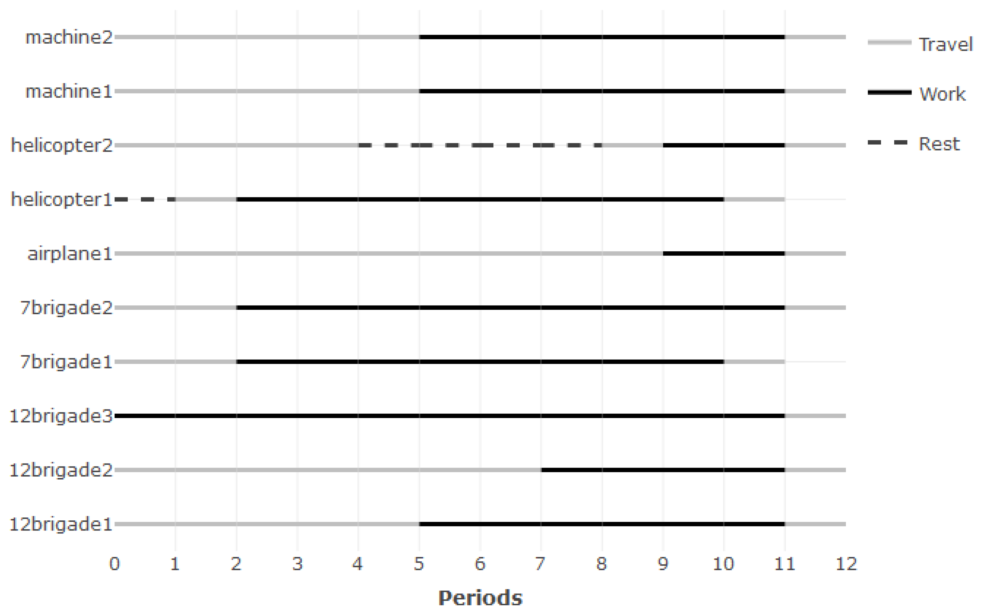
Running the model on our single fire test case, we obtain the fact that ten resources are selected to work to contain the fire (Figure 1). Helicopter1 and 12brigade3 continue to work to contain the fire, with the situation of the helicopter1 being particular because it is currently in a rest period. By contrast, airplane2 (no airplane2 is shown in Figure 1) finishes its work to contain the fire because it is longer favorable to incorporate a new resource.

With the optimal solution proposed by the mathematical model, it would be possible to contain the fire in period 11 with a total cost of 25,440 euros.

3.2. Results of the Simulations

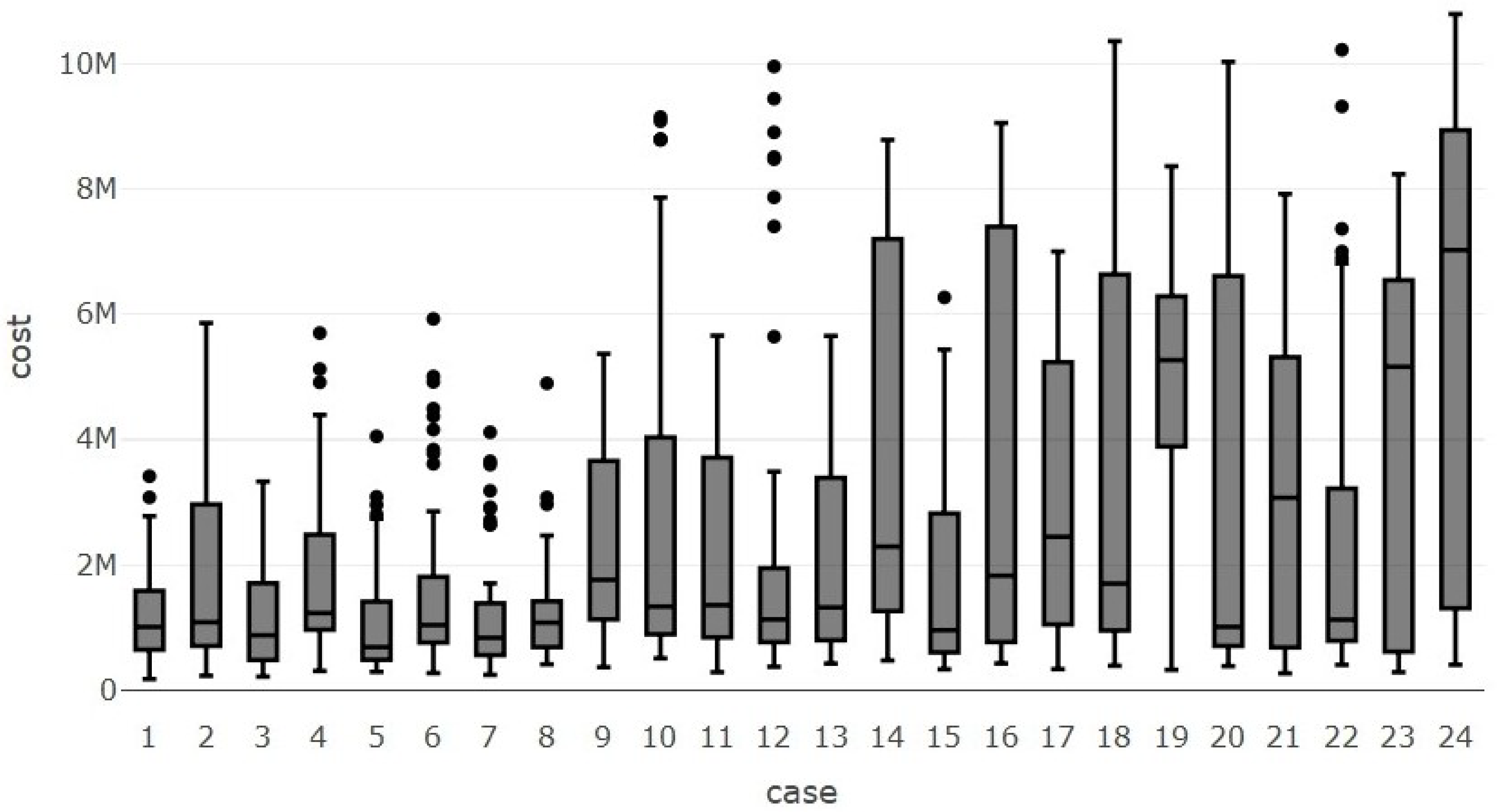
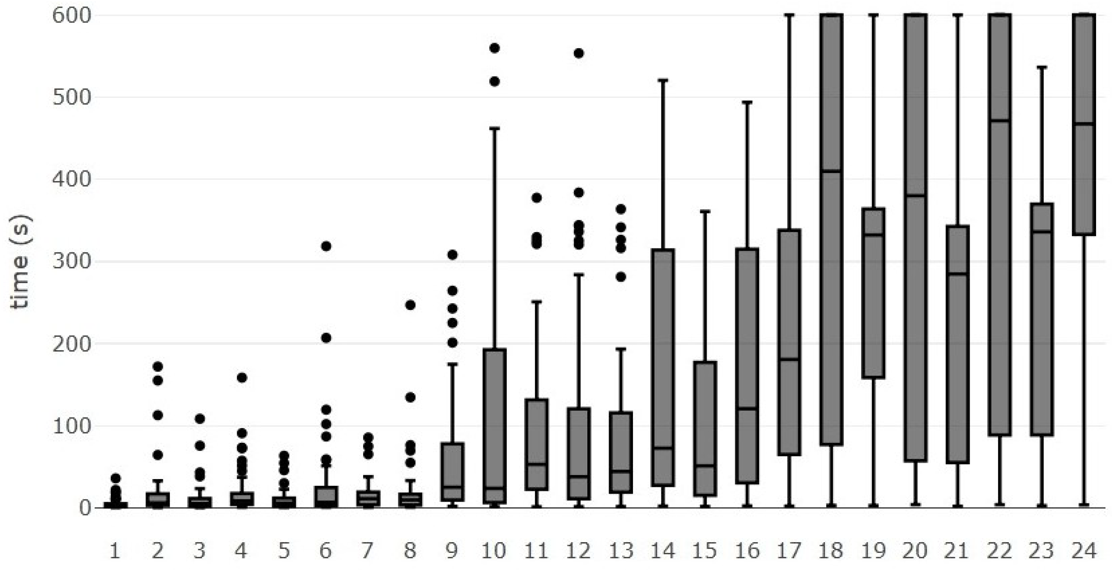
With respect to the spread of costs for each simulation case and the spread of execution times, the average cost and time to solve generally increase as the number of periods tested in the cases increase (Figure 2 and Figure 3). Variability in cost and time to solve also increase as the number of periods increase.

When we analyze the percentage of solved instances for each case (Figure 4), first we consider the percentage of instances that were resolved optimally with the first model. If the solver returned an infeasible or time_limit while executing the first model, the second model was used. We use the term optimal because, in the instances resolved with the first model, the fire can be extinguished in the period considered. We also consider the percentage of instances that were solved either with the first model or with the second. Remember that the second model is used when the fire cannot be extinguished with the resources available in the period considered, so we limit ourselves to maximizing the performance of the resources. The model will have to be executed again until the fire is extinguished. If, in the second model, an instance was not resolved within the desired time, then it was considered that the model was not solved, and therefore the black bar does not reach 100%.

3.3. Interface

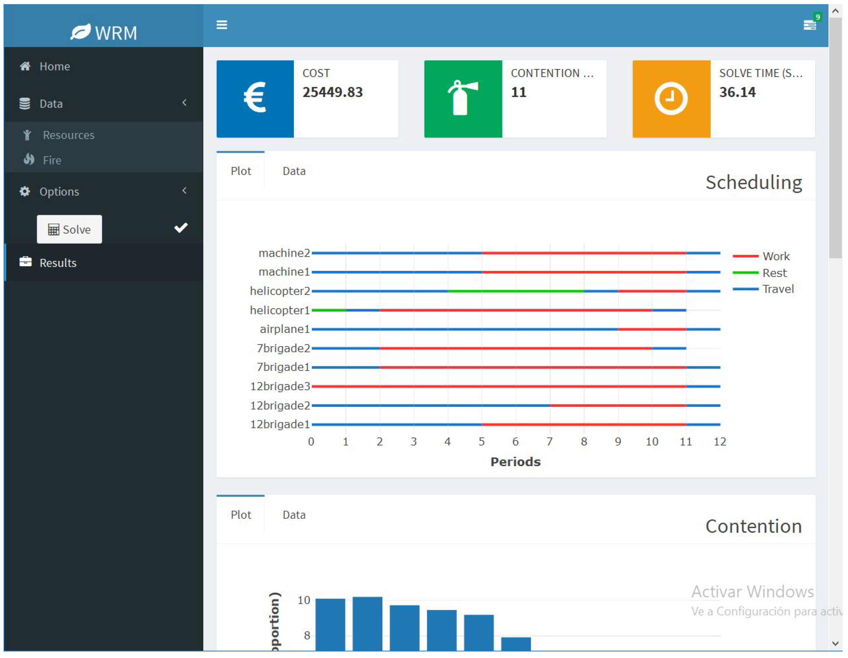
In order to execute the proposed model, we employ the wrm package [31], previously created with the software R. This open source package is stored on GitHub (a well-known web-based hosting service) and can be used to solve the mathematical model through an interface created with the shinydashboard [27] library (Figure 5).

The interface allows for simple interactions to load information on the resources as well as the evolution of the fire and aviation and brigade regulations. It also offers an option to run the model. Once the execution is complete, a visualization of the results is shown both graphically, which includes interactive graphics employing the plotly library [32], and in tabular format. It is possible to create HTML reports to save important information on the executed instance.

As we mentioned in the Introduction, at present, resource management combines the decisions made by the extinction coordinator with information contained and stored in a computer application. An automatic tool that allows one to visualize information like that provided by our interface is not available in the extinction services of Galicia, as far as we know.

4. Discussion

If we delve into the obtained results, the first issue that may draw our attention in our test case is the breach of the minimum number which is required for the different types of resources, specified in Section 2.3. However, non-compliance of the minimum number of resources only occurs in the initial periods because it is impossible to incorporate resources beforehand. On the other hand, it is observed in the test case that, in some periods, the maximum number of aircraft and brigades is reached. This does not happen with engines because their travel time to arrive at the location of the wildfire is very high. In this way, the results represent with a high degree of precision the results that appear in real life. It is also worth mentioning that the simulator constitutes an important support for the decisions taken in real fire management operations. This is so because it is responsible for feeding our models the parameters related to the expected evolution of the fire. In addition, the information on the evolution of the fire provided by the simulator is consistent with the forecast about the extinction provided by our model.

With respect to the simulations, it can be seen that the cost increases considerably when the number of periods increases. This is due to the possibility that the resources can increase their time of action, thus increasing the costs of their use and also the fire costs associated with those periods. However, for fire managers to interpret these results adequately, it must be taken into account that cases with fewer periods end up executing the modified model (and the fire is not really contained at the end of the period). The cost incurred is cheaper, but we must bear in mind that it is only the cost of the fire until the end of the period. The cost-per-period metric allows for easier comparisons of cost results, although for brevity this metric is not shown here.

We can see also that the smaller the number of periods, the shorter the runtime will be (Figure 3). Specifically, if the number of time periods is less than 30 (equivalent to 300 min), the execution times are small with all the instances being resolved in less than 10 min. If we analyze the execution times presented, it can be clearly observed that both the median and the variance for the execution time increases with a greater number of periods. To achieve consistently short executions times, we recommend performing executions with approximately 20 time periods (a time horizon of 3 h and 20 min).

In addition, it is not recommended to use more than 30 time periods as this would lead to a time horizon of five hours. An estimate with a longer time could be unreliable. This time is also recommended for achieving good estimates of the evolution of the fire. Since the model follows the rolling horizon philosophy, it is preferable to re-execute the model with fire conditions that are as real as possible, instead of running the model only once with a large time horizon. Since most fires take longer than five hours to extinguish, this would force the model to run more than once. Furthermore, since in the initial executions the fire could not be extinguished in the provided period, the model would initially be limited to maximizing the performance of the resources.

Regarding the instances of the simulations that have been solved, using the starting model or the modified model, we must point out that the Gurobi solver provides a local optimum of the problem. In some cases, the solver did not provide a local optimum with the execution time that was indicated. In this way, the solution could be obtained with a longer execution time. Specifically, regarding the gap of the integer programming problem, some unresolved instances were close to the optimum, while, in other instances, the time necessary to achieve the resolution would have had to be much greater. A future problem that we want to address is the design of new algorithms that allow a faster resolution of the model. At that time, we will conduct an exhaustive study of the gaps corresponding to unresolved instances with Gurobi.

As we mentioned in the Introduction, this model fits into the Enjambre project. It is not a stand-alone model, but the goal is to be part of a larger decision support system. This system includes different tools. We can highlight an anti-collision algorithm for air resources and an escape route algorithm for ground brigades. Other models relating to resources are two that attach aircraft to flight routes and aircraft to refueling points. We also have an algorithm used to detect obstacles for aircraft. We will also have a tool that represents the perimeter of the fire that we want to integrate with a simulator of the evolution of the fire. The use of these tools, in particular the evolution simulator of the fire, allows for updated information every time we execute our model (following the aforementioned rolling horizon methodology), on both the resources and the fire.

One issue with modeling forest fire extinction is the interaction between resource efforts and perimeter growth; as resources build a line around the fire, perimeter growth should be significantly slower than for a free-burning fire. See [33] for an example of an algorithm that deals with this. Our model adopts a pessimistic approach; we assume that the performance of resources does not mitigate the rate of evolution of the fire. The consequence is that, finally, the fire could be extinguished sooner than expected. However, the model indirectly interacts with perimeter growth and resource efforts. This is because the parameters of the model related to the fire come from simulations of its evolution, which also handle information from the line built by the resources.

The constant re-running of the model provides a desirable dynamic functionality [24]. Once decision makers select the desired response, the operation is monitored continuously and decisions are evaluated so that model adjustments can be made from time to time, in response to uncertain conditions which are characteristic of the fire environment. The decision process and results can be monitored and documented for the continuous learning of fire managers as well as the organizations on which they depend.

5. Conclusions

In this study, we develop a tool to facilitate the efficient assignment of resources to wildfires. The model incorporates mandated rest periods as well as restrictions arising from the non-negligence of fronts policy. The methodology used an integer linear programming model. Our simulation study showed that we can obtain an exact solution very quickly without the need to use heuristic algorithms, provided that the planning period does not exceed five hours. Thus, operations research can provide useful techniques for the management of resources in firefighting problems. We must emphasize that, in order to obtain useful research results, tools are needed to provide adequate values for model parameters and also historical fire data.

As future work, we believe that it is of interest to consider models with similar objectives and restrictions that consider the random nature of certain parameters. In addition, further work is needed on the design of new algorithms that make a faster resolution of the model feasible, and in this way enable optimal planning of the resources for a longer period of time, in a reasonable execution time. Lastly, in [34], a decision support tool was introduced to optimize the allocation of aerial resources for flight routes (circular paths that aerial resources follow such that they have common loading and discharge points) and refueling points. The integration of the model presented in this paper with that tool will also be a part of future work.

References

- Galicia, X. Consellería de Medio Rural. 2018. Available online: http://mediorural.xunta.gal/es (accessed on 18 June 2018).
- Galicia, X. PLADIGA: Memoria. 2017. Available online: http://mediorural.xunta.gal/fileadmin/arquivos/forestal/pladiga/2017/2$_$MEMORIA.pdf (accessed on 18 June 2018).
- Spanish Ministry of Development. Operational Circular 16-B. 1995. Available online: http://www.aecaweb.com/informes/documentos/INFORMES$_$Y$_$ESTUDIOS/circular$_$operativa$_$16$_$b.doc (accessed on 18 June 2018).
- Butry, D.T.; Mercer, E.; Prestemon, J.P.; Pye, J.M.; Holmes, T.P. What is the price of catastrophic wildfire? J. For. 2001, 99, 9–17. [Google Scholar]
- Schmuck, G.; San-Miguel-Ayanz, J.; Camia, A.; Oehler, F.; de Oliveira, S.S.; Durrant, T.; Kucera, J.; Boca, R.; Whitmore, C.; Giovando, C.; et al. Forest Fires in Europe 2008; Technical Report, European Commision EUR 23971 EN; OPOCE: Luxembourg, 2009; p. JRC53463. [Google Scholar]
- Arno, S.F.; Allison-Bunnell, S. Flames in Our Forest: Disaster or Renewal? Island Press: Washington, DC, USA, 2013. [Google Scholar]
- Martínez, J.; Vega-García, C.; Chuvieco, E. Human-caused wildfire risk rating for prevention planning in Spain. J. Environ. Manag. 2009, 90, 1241–1252. [Google Scholar] [CrossRef] [PubMed]
- Mavsar, R.; Cabán, A.G.; Varela, E. The state of development of fire management decision support systems in America and Europe. For. Policy Econ. 2013, 29, 45–55. [Google Scholar] [CrossRef]
- Martell, D.L. A review of recent forest and wildland fire management decision support systems research. Curr. For. Rep. 2015, 1, 128–137. [Google Scholar] [CrossRef]
- Headley, R. Fire Suppression, District 5; USDA-Forest Service: Washington, DC, USA, 1916; p. 57.
- Sparhawk, W.N. The Use of lIability Ratings in Planning Forest 28 Fire Protection; National Emergency Training Center: Emmitsburg, MD, USA, 1925. [Google Scholar]
- Gorte, J.K.; Gorte, R.W. Application of Economic Techniques to Fire Management-a Status Review and Evaluation; Gen. Tech. Rep. INT-GTR-53; U.S. Department of Agriculture, Forest Service, Intermountain Research Station: Ogden, UT, USA, 1979; p. 53.
- Donovan, G.H.; Rideout, D.B. A reformulation of the cost plus net value change (C+NVC) model of wildfire economics. For. Sci. 2003, 49, 318–323. [Google Scholar]
- Donovan, G.H.; Rideout, D.B. An integer programming model to optimize resource allocation for wildfire containment. For. Sci. 2003, 49, 331–335. [Google Scholar]
- Bilbao-Marón, M.N. Advanced Meta-Heuristic Approaches and Their Application to Operational Optimization in Forest Wildfire Management. Ph.D. Thesis, Universidad de Alcalá, Madrid, Spain, 2014. [Google Scholar]
- Lee, W.J. A Stochastic Mixed Integer Programming Approach to Wildfire Management Systems. Ph.D. Thesis, Department of Industrial and Systems Engineering, Texas A&M University, College Station, TX, USA, 2006. [Google Scholar]
- Hu, X.; Ntaimo, L. Integrated simulation and optimization for wildfire containment. ACM Trans. Model. Comput. Simul. (TOMACS) 2009, 19, 1–29. [Google Scholar] [CrossRef] [Green Version]
- Kim, Y.-H.; Bettinger, P. Spatial optimization of fuel management activities. In System Analysis in Forest Resources: Proceedings of the 2003 Symposium; General Technical Report, PNW-656; U.S. Department of Agriculture, Forest Service, Pacific Northwest Research Station: Portland, OR, USA, 2005; pp. 205–214. [Google Scholar]
- Kim, Y.-H.; Bettinger, P.; Finney, M. Spatial optimization of the pattern of fuel management activities and subsequent effects on simulated wildfires. Eur. J. Oper. Res. 2009, 197, 253–265. [Google Scholar] [CrossRef]
- Costafreda-Aumedes, S.; Cardil, A.; Molina, D.M.; Daniel, S.N.; Mavsar, R.; Vega-García, C. Analysis of factors influencing deployment of fire suppression resources in Spain using artificial neural networks. iFor.-Biogeosci. For. 2015, 9, 138–145. [Google Scholar] [CrossRef]
- Pappis, C.P.; Rachaniotis, N.P. Scheduling in a multiprocessor environment with deteriorating job processing times and decreasing values: The case of forest fires. J. Heuristics 2010, 16, 617–632. [Google Scholar] [CrossRef]
- Drozdowski, M. Real-time scheduling of linear speedup parallel tasks. Inf. Process. Lett. 1996, 57, 35–40. [Google Scholar] [CrossRef]
- Duff, T.J.; Tolhurst, K.G. Operational wildfire suppression modelling: A review evaluating development, state of the art and future directions. Int. J. Wildl. Fire 2015, 24, 735–748. [Google Scholar] [CrossRef]
- Dunn, C.J.; Thompson, M.P.; Calkin, D.E. A framework for developing safe and effective large-fire response in a new fire management paradigm. For. Ecol. Manag. 2017, 404, 184–196. [Google Scholar] [CrossRef]
- R Core Team. R: A Language and Environment for Statistical Computing; R Foundation for Statistical Computing: Vienna, Austria, 2017. [Google Scholar]
- Gurobi Optimization, Inc. Gurobi Optimizer Reference Manual; Gurobi Optimization, Inc.: Beaverton, OR, USA, 2016. [Google Scholar]
- Chang, W.; Borges Ribeiro, B. Shinydashboard: Create Dashboards with ‘Shiny’. R Package Version 0.7.0. 2018. Available online: http://rstudio.github.io/shinydashboard/ (accessed on 19 september 2018).
- Silva, R.F. Coste y eficiencia en las operaciones de extinción de incendios forestales. Fundamentos y herramientas para su estudio y análisis. In Proceedings of the 4th International Wildland Fire Conference, Seville, Spain, 14–17 May 2007. [Google Scholar]
- Silva, R.F.; González-Cabán, A. Contribution of suppression difficulty and lessons learned in forecasting fire suppression operations productivity: A methodological approach. J. For. Econ. 2016, 25, 149–159. [Google Scholar]
- Vázquez, M.C.V.; Amil, M.L.C.; Montero, J.M.T. Estimación de los costes de las operaciones de extinción de incendios forestales: Estudio de caso en el distrito forestal de A Limia. Rev. Galega Econ. 2015, 23, 99–114. [Google Scholar]
- Rodríguez-Veiga, J.; Ginzo-Villamayor, M.J.; Casas-Méndez, B. Wildfire Resources Management (wrm). 2018. GitHub Repository. Available online: https://github.com/jorgerodriguezveiga/wrm (accessed on 19 September 2018).
- Sievert, C.; Parmer, C.; Hocking, T.; Chamberlain, S.; Ram, K.; Corvellec, M.; Despouy, P. Plotly: Create Interactive Web Graphics via ‘plotly.js’. R Package Version 4.7.1. 2017. Available online: https://rdrr.io/cran/plotly/ (accessed on 19 september 2018).
- Fried, J.S.; Fried, B.D. Simulating wildfire containment with realistic tactics. For. Sci. 1996, 42, 267–281. [Google Scholar]
- Rodríguez-Veiga, J.; Gómez-Costa, I.; Ginzo-Villamayor, M.J.; Casas-Méndez, B.; Sáiz-Díaz, J.L. Assignment Problems in Wildfire Suppression: Models for Optimization of Aerial Resource Logistics. For. Sci. Available online: http://dx.doi.org/10.1093/forsci/fxy012 (accessed on 18 June 2018).
Figure 1.
Scheduling of selected resources to fight the test wildfire.
Figure 2.
Distribution of the total cost for each case over 50 simulation instances.
Figure 3.
Distribution of the execution time for each case over 50 simulation instances.
Figure 4.
Percentage of solved instances for each case, with the main model (gray bar) or with one of the two models (black bar).
Figure 5.
View of typical results for an instance run with the interface wrm package in software R.