Estimation of Forest Above-Ground Biomass by Geographically Weighted Regression and Machine Learning with Sentinel Imagery


1
Key Laboratory of Wetland Ecology and Environment, Northeast Institute of Geography and Agroecology, Chinese Academy of Sciences, Changchun 130102, China
2
University of Chinese Academy of Sciences, Beijing 100049, China
*
Author to whom correspondence should be addressed.
Forests 2018, 9(10), 582; https://doi.org/10.3390/f9100582
Submission received: 31 August 2018
/
Revised: 12 September 2018
/
Accepted: 19 September 2018
/
Published: 20 September 2018
(This article belongs to the Special Issue Remote Sensing Technology Applications in Forestry and REDD+)
Abstract
:Accurate forest above-ground biomass (AGB) is crucial for sustaining forest management and mitigating climate change to support REDD+ (reducing emissions from deforestation and forest degradation, plus the sustainable management of forests, and the conservation and enhancement of forest carbon stocks) processes. Recently launched Sentinel imagery offers a new opportunity for forest AGB mapping and monitoring. In this study, texture characteristics and backscatter coefficients of Sentinel-1, in addition to multispectral bands, vegetation indices, and biophysical variables of Sentinal-2, based on 56 measured AGB samples in the center of the Changbai Mountains, China, were used to develop biomass prediction models through geographically weighted regression (GWR) and machine learning (ML) algorithms, such as the artificial neural network (ANN), support vector machine for regression (SVR), and random forest (RF). The results showed that texture characteristics and vegetation biophysical variables were the most important predictors. SVR was the best method for predicting and mapping the patterns of AGB in the study site with limited samples, whose mean error, mean absolute error, root mean square error, and correlation coefficient were 4 × 10⁻³, 0.07, 0.08 Mg·ha−1, and 1, respectively. Predicted values of AGB from four models ranged from 11.80 to 324.12 Mg·ha−1, and those for broadleaved deciduous forests were the most accurate, while those for AGB above 160 Mg·ha−1 were the least accurate. The study demonstrated encouraging results in forest AGB mapping of the normal vegetated area using the freely accessible and high-resolution Sentinel imagery, based on ML techniques.
1. Introduction
As the largest carbon sinks on land, forest ecosystems account for about 80% of terrestrial biosphere carbon storage, and play a pivotal role in mitigating climate change [1,2]. Above-ground biomass (AGB), accounting for between 70% and 90% of total forests biomass [3], is one of the important carbon pools in forest ecosystems, and it is a key indicator of forest vegetal health, as well as related seral stages [4,5]. The spatially explicit measurement of forests’ AGB also supports REDD+ (reducing emissions from deforestation and forest degradation, plus the sustainable management of forests, and the conservation and enhancement of forest carbon stocks) processes [6]. Therefore, the rapid and accurate estimation and monitoring of AGB over various scales of space and time are crucial for greatly reducing the uncertainty in carbon stock assessments, and for informing strategic forest management plans [7,8,9].
Traditional field-based measurements provide the most accurate AGB values, but they are destructive and spatially limited [10,11]. Uncertainty and bias in field measurements obviously exist, particularly those with large trees and tropical issues [4,5]. Combining remote sensing and sample plot data has become a popular method to generate spatially explicit estimations of forest AGB [12,13]. Various types of remote-sensing data are used for forest biomass estimation such as optical sensor data, radio detection and ranging (radar) data, and light detection and ranging (LiDAR) data, with each one having certain advantages over the others [14,15]. Optical sensors were first applied to retrieve the horizontal forest structure and AGB assessments through field sampling, due to their aggregate spectral signatures (reflectance or vegetation indices) with global coverage, repetitiveness, and cost-effectiveness [16,17]. Optical remote sensing data from a number of platforms, such as IKONOS, Quickbird, Worldview, ZY-3, systeme probatoire d’observation de la terre (SPOT), Sentinel, Landsat, and moderate-resolution imaging spectroradiometer (MODIS), with spatial resolutions varying from less than one meter to hundreds of meters, have been used by numerous researchers for biomass estimation [18,19,20]. However, the widespread usage of optical data is limited by its poor penetration capacity through clouds and forest canopies, as well as data saturation problems [21]. Radar data, available internationally from airborne or space-borne systems with different frequency bands, polarizations, and variable imaging geometries, such as Terra-SAR (Terra-Synthetic Aperture Radar), advanced land observing satellite phased array L-band synthetic aperture radar (ALOS PALSAR), and Sentinel, have gained prominence for AGB estimation because of their better penetration ability and detailed vegetation structural information, but these still suffer from signal saturation problems [6,14,22]. LiDAR, an active remote-sensing technology, captures forests’ vertical structures in great detail and provides 3D information, such as the geoscience laser altimeter system (GLAS), which has found favor in biomass estimation with an improved accuracy, but with complex data-processing, and the lack of space continuity problems [23,24]. Additionally, some research using 3-D terrestrial LiDAR has shown bias in biomass, especially from tropical species, mainly because of the underestimation of tree height [25,26]. In other words, the accuracy of forest AGB estimates could be improved by a combined use of multi-source remote sensing data. The above-mentioned Sentinel satellite constellation series, including the Sentinel-1 C-band Synthetic Aperture Radar (SAR) and the Sentinel-2 multispectral instrument by the European Space Agency (ESA), provide new capabilities for AGB mapping with wide coverage, a short return cycle, and a long lifespan as the same data format [27,28,29]. In other words, the Sentinel series may have a high synergetic potential for overcoming the limitation of single remote sensing techniques for forest AGB estimation. The Sentinel imagery have been applied in a number of previous vegetation studies, focusing on classification [30,31,32], vegetation parameters on agricultural fields [33,34,35], grassland [36,37,38], and forests [39,40], as well as the damage extent of disasters [41,42,43], while forest AGB mapping based on Sentinel imagery is still insufficient.
The techniques for estimating forests’ AGB based on remote sensing data have allowed for ‘scale-up’ or extrapolation of the field data collected for larger scales [8,44]. It is a predictive mapping process for an estimation of the value at a location without direct observation. It depends on the values of points at nearby sites where observations were made, and/or values of other factors at the sites, through various methods. Those methods can be divided into two categories: parametric and non-parametric algorithms [45,46]. The former refers to statistical regression methods, such as the stepwise regression models (SWR) and geographically weighted regression (GWR), by which the expression relating to the dependent variable (AGB) and the independent variables is easy to calculate [2]. However, there is no simple global linear relationship like the SWR model, between remote sensing data and forest AGB, because it is affected by many factors. The GWR method explores spatial heterogeneity, as well as the non-stationarity of relationships, and it estimates the parameters for each sample location, which makes it a very attractive tool for remotely-sensed biomass modeling [47,48]. Non-parametric techniques, including machine learning (ML) methods such as the k-nearest neighbor (KNN), artificial neural network (ANN), support vector machine for regression (SVR), and random forest (RF), have a better ability for identifying complex relationships between predictors and the forest AGB [2,49]. Despite a variety of forest AGB models, quite a few research studies merely focused on one parametric or non-parametric model are unpersuasive. Thus, a systematic comparison of GWR, ANN, SVR, and RF for mapping forest AGB based on Sentinel imagery is fairly urgent, but also rare in the literature.
In this study, the ability of Sentinel-1 and Sentinel-2 imagery for the retrieval and predictive mapping of forests’ AGB estimation was evaluated. The specific objectives included the following: (1) to determine and model the relationship between field-measured forests AGB and Sentinel-based predictors, including Sentinel-1 SAR backscatter information and Sentinel-2 multispectral indices based on GWR and ML; (2) to evaluate and compare the accuracy of the biomass prediction models, including GWR, ANN, SVR, and RF models; and (3) to map forest AGB spatial distribution by four optimal models. The novelty of this paper is the use of Sentinel-1 (texture characteristics and backscatter coefficients) and Sentinel-2 (multispectral bands, vegetation indices, and biophysical variables) imagery in the mapping of forest AGB and AGB model development, as well as their comparison. This study attempted to contribute to the development of remote sensing-based predictive mapping techniques for forest AGB using freely accessible multi-source remote sensing data with a relatively high spatial resolution.
2. Materials and Methods
2.1. Study Site
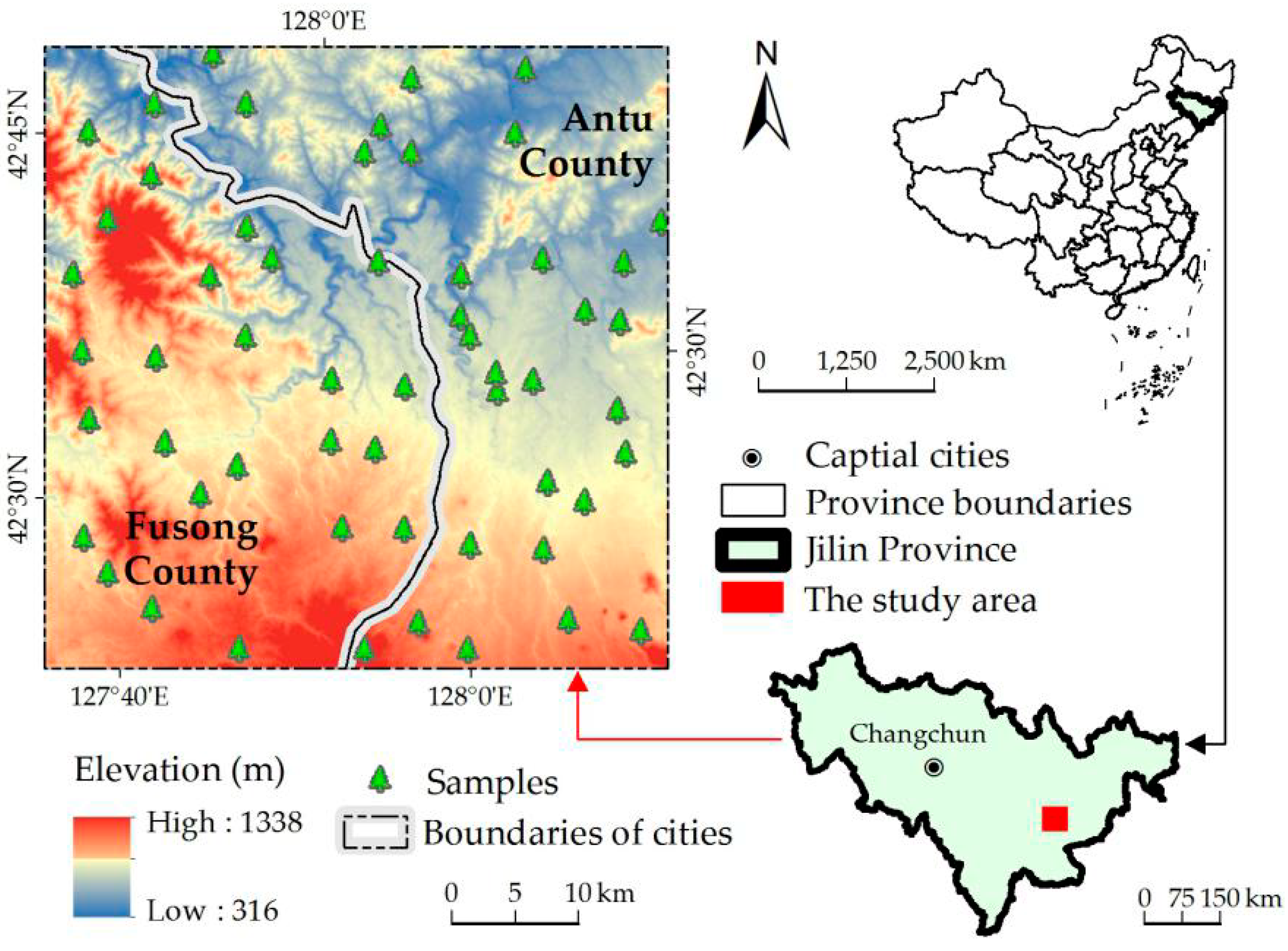
This study was conducted in a sample area (42°17′–42°49′ N, 127°35′–128°20′ E), which spanned over 2500 km2. It is located in the southeast region of Jilin Province, northeast China, in the center of the Changbai Mountains (Figure 1). The study area consists of five towns: Yanjiang and Lushuihe towns of the Fusong County of Baishan City; and Yongqing, Liangjiang, and Erdaobaihe towns of the Antu County of the Yanbian Korean Autonomous Prefecture. This area has a northern temperate continental monsoon climate, with an annual average temperature of 2.8 °C and an annual precipitation of 8000 mm [50,51]. Characterized by high forest cover, the spatial distribution of forest types in the study area obtains obvious vertical zonality, with Pinus koraiensis Sieb. et Zucc., Larix gmelinii var. japonica, Betula platyphylla Suk., Fraxinus mandschurica Rupr., and Juglans mandshurica Maxim. as typical tree species [51].
2.2. Field Observations
The field campaign was conducted from July to August, 2017. Before that, the distribution of sampling plots was generated using ArcGIS (version 10.0, ESRI, RedLands, CA, USA), with the non-forest area being masked out. Non-forested areas were derived from 2015 land use and a land cover map [52] by visual interpretation and manual modification based on Sentinel-2 images (Table 1). In the field, nearby preset plots, a total of 56 sampling quadrats measuring 10 m × 10 m were laid out at each representative sampling plot (Figure 1), including two evergreen coniferous forests, 30 broadleaved deciduous forests, five deciduous coniferous forests, and 19 mixed broadleaf-conifer forests.
The sampling equipment were the diameter at breast height ruler for measuring the diameter at 1.3 m from the ground and the laser altimeter (TruPulse200, Laser Technology Inc., Norristown, PA, USA) for the tree height measurement. Based on allometric equations (Table 2), some AGB are the sum of tree trunks, branches, and leaf biomass, and others are directly calculated by diameters at breast height (cm) and tree height (m). The AGB of 56 samples ranged from 14.64~317.40 Mg·ha−1, with mean and median values of 80.44 and 66.00 Mg·ha−1, respectively.
2.3. Satellite Data Pre-Processing and Predictors Derived
Sentinel-1 Synthetic Aperture Radar (SAR) and cloud-free Sentinel-2 multispectral imagery from the European Space Agency used in this study (Table 1) were downloaded from the agency’s Copernicus Sentinel Scientific Data Hub (https://scihub.copernicus.eu/dhus/#/home). Sentinel-1 C-band images adopted in this study were collected in the interferometric wide swath mode of the VH (vertical transmit-Horizontal receive) and VV (vertical transmit-vertical receive) polarizations. With a pixel size of 10 m, the SAR images are at a high-resolution (HR) Level-1 ground range detected (GRD) processing level. The Sentinel-2 Level 1C data involved were top-of-atmosphere reflectance images, and they were processed for orthorectification and spatial registration. The imagery had 13 spectral bands in the visible, near infrared, and short-wave infrared regions, and had 10 m (band 2–4, 8), 20 m (band 5–7, 8a, 11–12), and 60 m (band1, 9–10) spatial resolutions. In addition, elevation data (30 m) from the Shuttle Radar Topography Mission (SRTM) product was acquired from the United States Geological Service’s Earth Explorer (https://earthexplorer.usgs.gov/) for inclusion in the analysis of the Sentinel imagery [55].
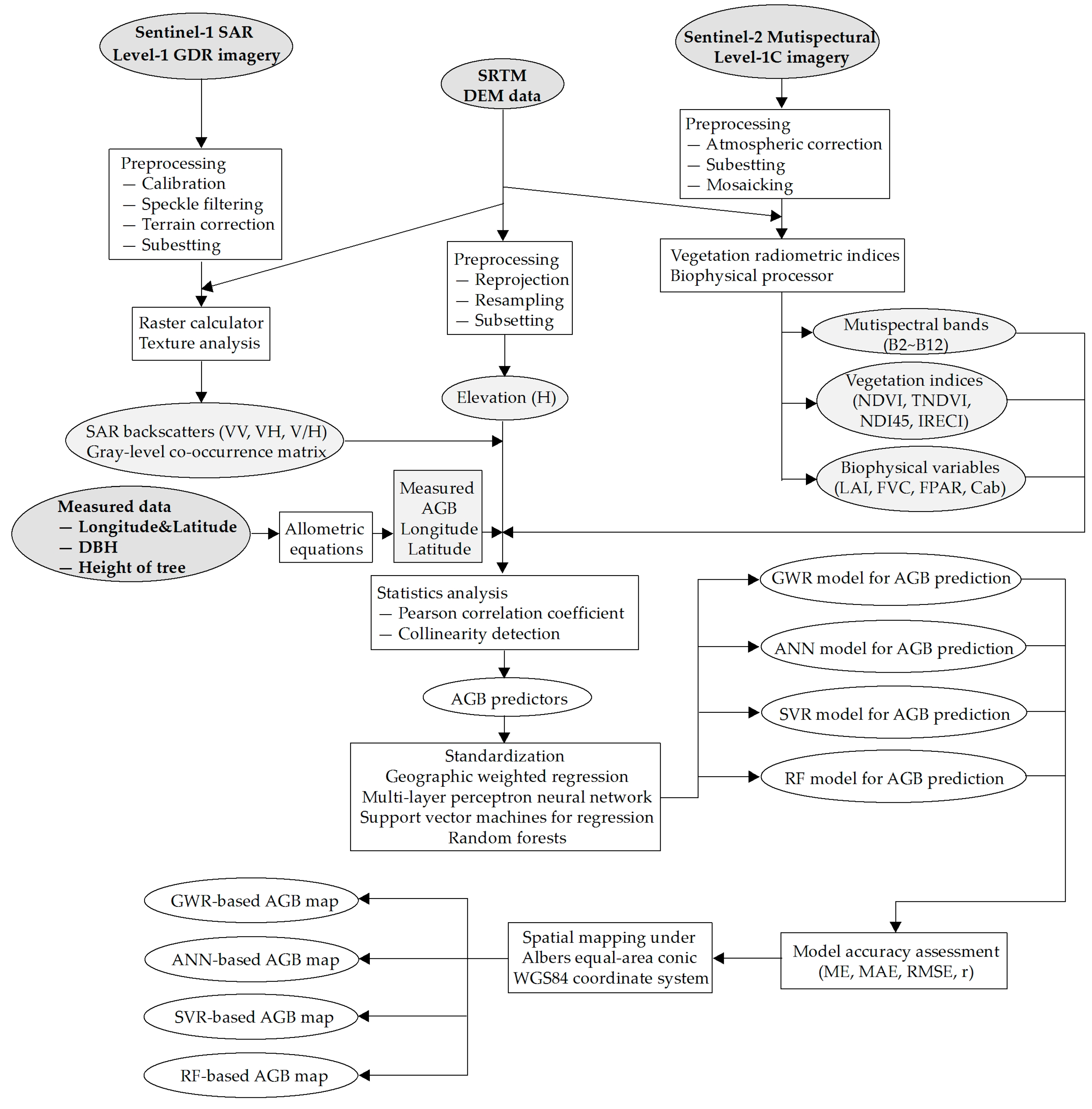
The processing steps used in the study are summarized in Figure 2. Sentinel application platform (SNAP) software (version 6.0, European Space Agency) was used to pre-process Sentinel-1 and Sentinel-2 imagery. The steps for the SAR imagery based on the Sentinel-1 Toolbox consisted of image calibration, speckle reduction using the Refined Lee Filter, and terrain correction using the Range-Doppler to acquire an accurate radar intensity backscatter coefficient with a map projection [56,57]. Multispectral imagery was atmospherically corrected and processed by the radiative transfer model-based Sen2Cor atmospheric correction processor (version 2.5.5, European Space Agency) to a Level-2A product, a bottom-of-atmosphere-corrected reflectance image. The pre-processed Sentinel images, as well as the elevation data, were brought into a common map projection, universal transverse mercator (UTM) Zone 52 WGS84, and resampled to 10 m pixel sizes. Subsetting and mosaicking were done to cover the study area.
In this study, 44 predictors were selected and extracted according to previous research [55,58]. Shown in Table 3, 23 predictors were from Sentinel-1 and 18 variables were from Sentinel-2, as well as elevation (H) from SRTM. Additionally, the other two variables were longitude and latitude. The first and second part derived from the Sentinel-1 imagery consisted of relating the field AGB with Sentinel SAR polarization channels, and their calculation and texture characteristics. The third to fifth parts based on the Sentinel-2 images proceeded with relating the field AGB to the multispectral bands, vegetation indices, and biophysical variables. The biophysical variables were also calculated in SNAP from its biophysical processor, which uses a neural network algorithm based on the PROSPECT+SAIL (PROSAIL) radiative transfer model [59]. Except for serving as a predictor, the elevation data from SRTM digital elevation model (DEM) were supplemented with Sentinel imagery processing to improve the accuracy (Figure 2).
3. Modeling the Relationship between Field AGB and Satellite Data
Firstly, the pairwise Pearson’s product-moment correlation analysis was conducted to determine the correlation of observed above-ground biomass and Sentinel-based predictors, as well as the collinearity between predictors. Predictors that were highly correlated to each other (r ≥ 0.8), and had high variance inflation factors (VIFs ≥ 10) in regression analysis, were excluded from modeling [65,66]. These analysis steps were performed using SPSS (version 21.0, IBM, Armonk, NY, USA). Then, all of the explanatory variables were transformed to a Z-score to eliminate the effect of index dimension and quantity of data. The formula was defined as x* = (x − μ)/σ, where μ is the mean value of a specific explanatory variable and σ is its standard deviation [67]. After that, GWR, ANN, SVR, and RF were used in this study to model ABG based on Sentinel-derived predictors (Figure 2).
3.1. Geographically Weighted Regression
Originally proposed by Brunsdon et al. (1998), GWR is a powerful approach for modeling spatially heterogeneous processes at a local scale [68,69,70]. It estimates the individual parameters for each estimation location, and the parameter estimation at any location obeys the distance decay. In other words, the closer to the location of an observation, the greater the weight that is allotted for the observation. The GWR form is regularly expressed as [47]:
where is the dependent variable value of observation i considered in the parameter estimation at the location (ui, vi); β0(ui, vi) is the intercept; βk(ui, vi) is the coefficient of k explanatory variables, indicating a parameter estimate that explains the relationship around location (ui, vi), which varies with the location; x*ik represents the independent variables of observation i; p is the total number of explanatory variables; and εi is the error term that is generally assumed to be explanatory and normally distributed with zero mean and constant variance. The parameter estimator βk(ui, vi) is identical to the weighted least squares regression, where the weights are computed based on the distance between the observations [48]. The parameters are estimated as [71]:
where X is the matrix formed by x*ik; Y is the vector formed by values of the dependent variables; W(ui, vi) is a weight matrix to ensure that those observations near the point i have more influence on the results than those farther away; and the weights are calculated based on a kernel weighting scheme such as fixed Gaussian, fixed bi-square, adaptive bi-square, and adaptive Gaussian [72]. In this study, we used the fixed Gaussian kernel as [73]:
where di(ui, vi) is the distance between the observation i and the location (ui, vi); and h is a quantity called bandwidth, which controls the effect of the distance on the weight value.
GWR was conducted using GWR (version 4.0, Ritsumeikan University, Kyoto, Japan), by which the weight function (a geographic kernel type) and the minimum value of the corrected Akaike information criterion (AICc, small sample bias corrected AIC) are determined to find the optimal bandwidth by a golden section search [74].
3.2. Machine Learning Methods
The machine learning methods adopted in this study were modeled in WEKA software (version 3.8, The University of Waikato, Hamilton, New Zealand). The models defined the best parameters with the highest correlation coefficient (r) and the lowest root mean square error (RMSE) for the prediction of AGB, and then AGB mapping was implemented in ArcGIS.
3.2.1. Multi-Layer Perception Neural Network
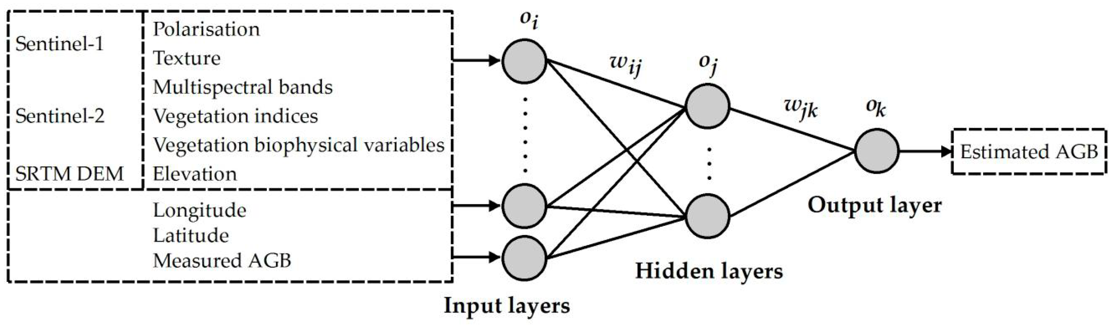
As a nonparametric mathematical model, ANN is inspired by biological neural networks and it has strong abilities for linear and nonlinear fitting [75,76]. The ANN considered in this study was the multi-layer perception neural network (MLPNN). The architecture of the MLPNN consists of an input layer containing predictors, one or more hidden layers, and an output layer containing the response variable, along with interconnection weights characterizing the connection strength between these layers (Figure 3). The algorithm chosen was the back-propagation (BP) learning rule, an iterative gradient descent algorithm that was designed to minimize the mean square error between the desired target and the actual output vectors [77,78]. The initial weights were assigned randomly, and when developing the network, the interconnection weights were adjusted to minimize the prediction error [79,80].
3.2.2. Support Vector Machines for Regression
SVR is a regression version of support vector machines that project the training dataset from a lower dimensional space into a higher dimensional feature space using kernel functions to separate groups of input data in a linearized manner, based on the Vapnik-Chervonenkis (VC) dimension theory and structural risk minimization [81,82,83]. An SVR function for AGB estimation is defined as [84]:
where x is a vector of the input predictors; K(xk, xj) is a kernel function; b is a constant threshold; and αk and are the weights (Lagrange multipliers), with the constraints given in Equation (5):
where C is the regularization parameter for balancing between the training error and model complexity. The sequential minimal optimization (SMO) algorithm was used to solve the quadratic programming optimization problem step-by-step and to update Equation (4) to reflect the new values until the Lagrange multipliers converged [66,85].
Among the various kernel functions, the radial basis function (RBF) shows a superior performance and robust results [86,87], and was used in this study [88]:
where σ is a scale parameter chosen based on the training data, and a unit vector could be concatenated with kernels as the intercept. In a word, the training of the SVR model required finding the best values for the two meta-parameters: the regularization parameter (C) and the kernel width (σ).
3.2.3. Random Forests
As a classification and regression tree (CART) technique proposed by Breiman (2001), RF combines bagging [89,90] with random variable selections at each node [91] to iteratively generate a large group of CARTs. The classification output represents a majority vote (classification), or an average (regression) from the whole ensemble, and hence achieves a more robust model than a single classification tree that is produced by a single model run [89,92,93]. A number of decision trees in RF choose their best splitting attributes from a random subset of predictors at each internal node without pruning. Based on the bootstrap sampling procedure, RF ensures at the same time the smallest obtainable bias and very low data variance [94]. There are two main important parameters: numFeatures, which means the number of features for splitting the nodes, whose default value is int[ln(numbers of predictors) + 1] in WEKA; and numIterations, which means the number of trees to be optimized in the modeling process, depending on specific application objectives [95].
3.3. Evaluation of ABG Models
4. Results
4.1. Statistics Analysis
The poor correlation of the observed AGB and the predictors was acquired from the low value of r (−0.288–0.263). Among predictors, VV_MAX (r = −0.288), VV_ENE (r = −0.284), VV_HOM (r = −0.277), VV_ASM (r = −0.276), and VV_ENT (r = 0.263) were significantly correlated (p-values < 0.05) with AGB. Predictors from the texture characteristics of Sentinel-1 VV polarization were significantly associated with AGB, as similarly found by Pan and Sun (2018) [58]. Those r values represent an average global correlation; thus, it also indicated that the global linear regression was inappropriate for AGB modeling in this study.
Among the 44 explanatory variables, VV_ASM (rvv_ASM,MAX = 0.99, VIFs = 41.3), VV_ENE (rvv_ENE,MAX = 0.995, VIFs = 106.8), VV_ENT (rvv_ENT,MAX = −0.97, VIFs = 18.2), and VV_HOM (rvv_HOM,MAX = 0.98, VIFs = 20.1) were excluded from model building because their VIFs exceeded the above-mentioned threshold (VIFs ≥ 10), and this reduced the number of explanatory variables from 44 to 40.
4.2. Models of GWR and ML
The optimal bandwidth for GWR in this study was 0.023, with the minimum value of AICc being 694.91, and the adjusted R2 of this GWR model being 0.79. For a given environmental variable, its coefficient from GWR varied across the study area. The top five predictors for the mean magnitude of the coefficients were VV_MEA (16.5, negative), VV_VAR (16.1, positive), LAI (1.6, positive), Cab (0.9, positive), and FVC (Fraction of Vegetation Cover) (0.8, positive). Predictors from the texture characteristics of Sentinel-1 VV polarization and the vegetation biophysical variables of Sentinel-2 showed a relatively strong association with AGB at a local regression.
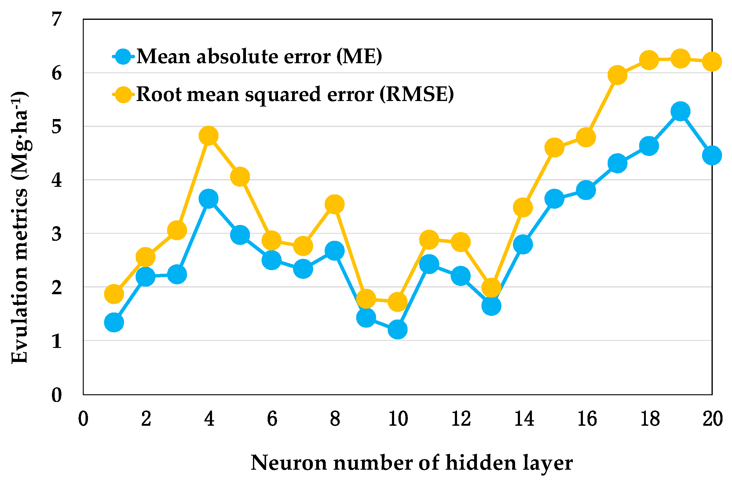
As for the MLPNN model, the accuracy for various numbers of neurons in the hidden layer is shown in Figure 4. The results revealed that the optimized MLPNN architecture was 40-10-1, indicating that there were 40 input nodes in the input layer, 10 nodes in the hidden layer with the unipolar sigmoid as the transfer function, and one node in the output layer. Using the Levenberg-Marquardt learning algorithm, the best learning rate, momentum, and training time (iterations) obtained were determined to be 0.2, 0.3, and 500, respectively. In the SVR model, the best parameters C and σ obtained were 1 and 2, respectively. With iteration (trees) numbers of 50 and feature numbers of 5, the top five predictors for attribute importance in the selected RF model were VV_CON, VH_HOM, VH_DIS, VH_ASM, and VH_ENT. The texture characteristics of Sentinel-1 VV and VH polarizations were relatively vital for modeling AGB by RF in this study.
4.3. Models Evaluation and Mapping of AGB
4.3.1. Models Assessment by Evaluation Indices
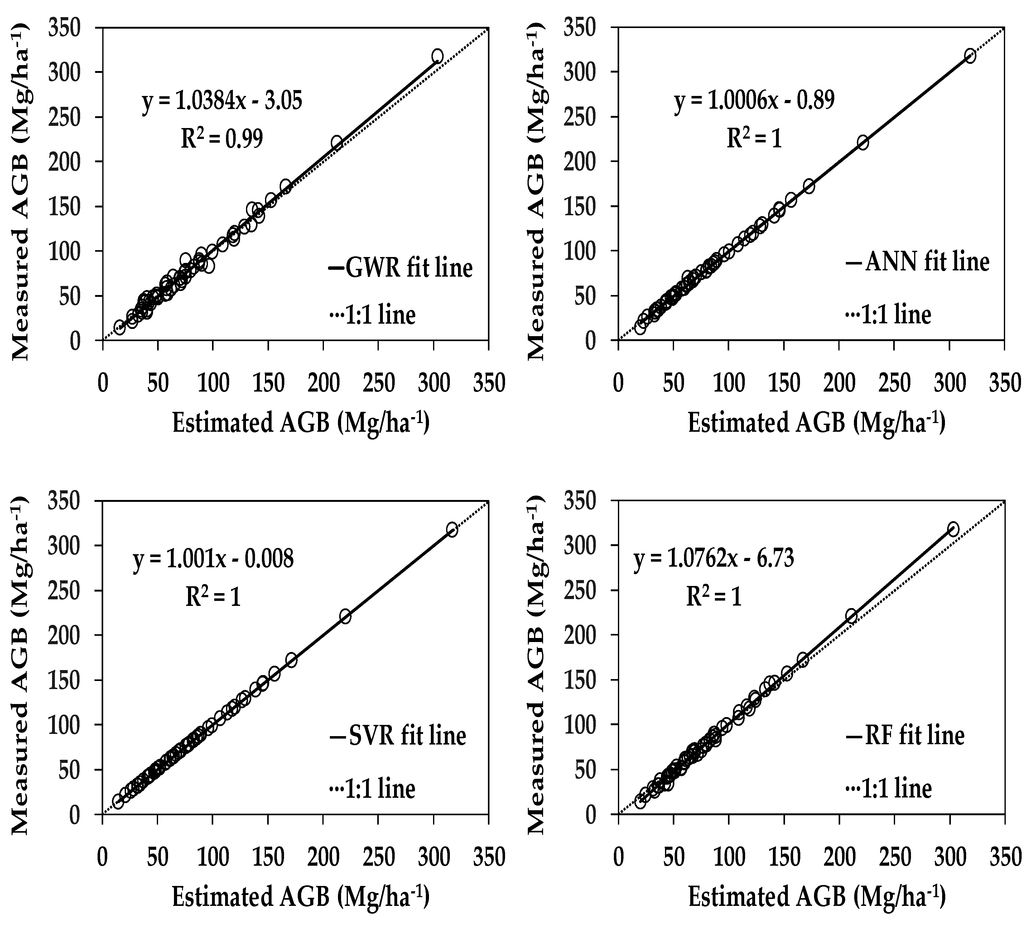
Table 4 presents the accuracies of four models for estimating the AGB of 56 forest quadrats. All four models overestimated the AGB. The ANN model resulted in an ME of 0.84 Mg·ha−1, and had the highest tendency for overestimation; the SVR model with an ME of 0.004 Mg·ha−1 showed the lowest tendency for overestimation. The MAE, indicating the extent to which the process leads to error, was lower with SVR (0.07 Mg·ha−1), and higher with the other methods, ranging from 1.21 (ANN) to 4.01 Mg·ha−1 (GWR). The values of the RMSE suggested that ML methods, whose RMSE ranged from 0.08 (SVR) to 4.43 (RF) Mg·ha−1, produced less error than GWR. A better consistency between the measured AGB and the estimated one was discovered by the r values from the ML models (0.999 of RF to 1 of SVR and ANN) compared to the GWR model (0.995). The SVR model gave rise to the lowest RMSE and the closest-to-zero ME and MAE values, as well as the highest r value. Hence, in this study, the SVR model was the most accurate model for estimating AGB. Besides, the accuracy ranking of the four methods from high to low was SVR, ANN, RF, and GWR. To further analyze the modeling accuracy, the estimated values of AGB were plotted against the measured values (Figure 5). An estimation from the SVR model showed the best agreement along the 1:1 line, followed by those from ANN, GWR, and RF.
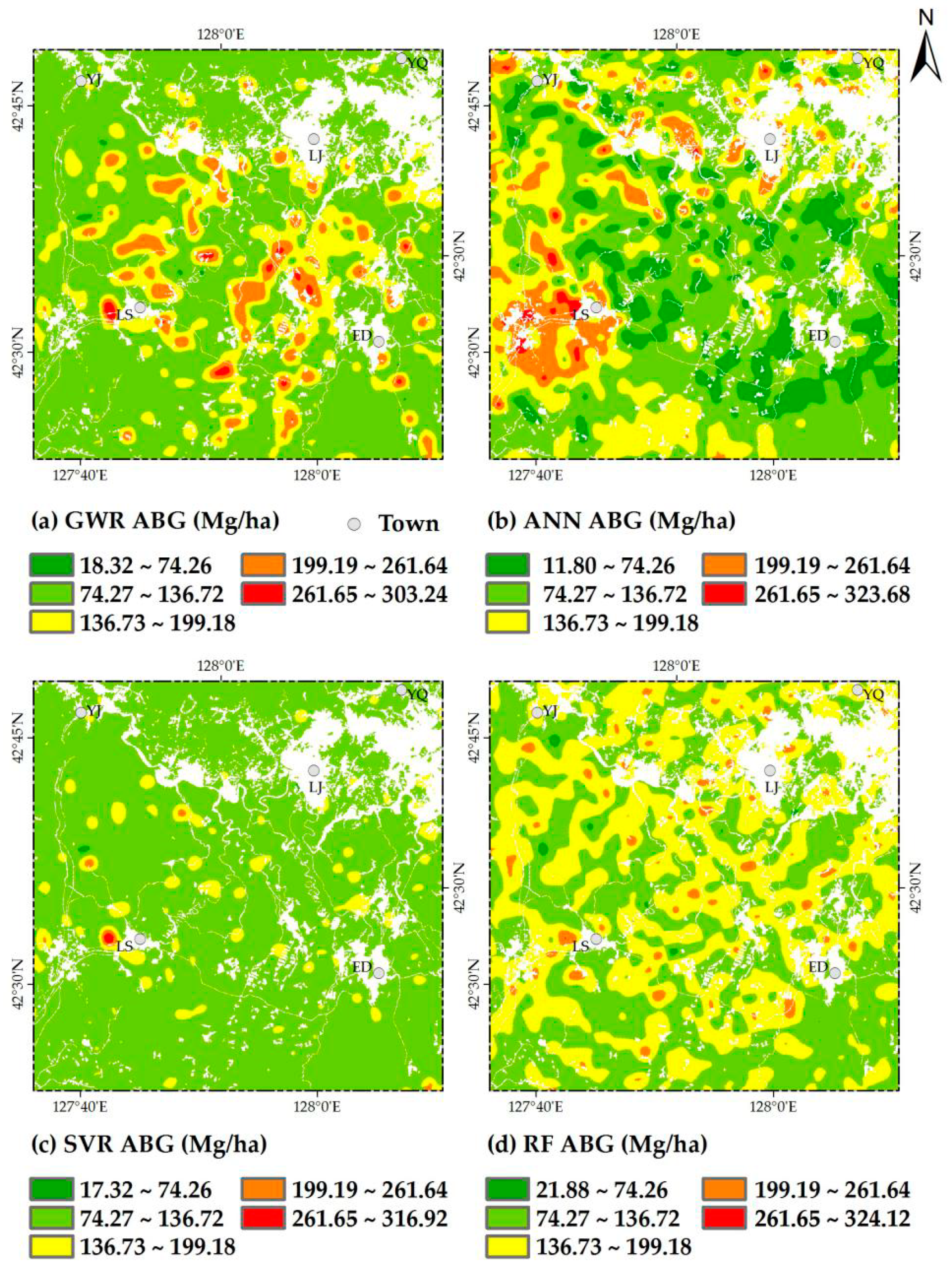
4.3.2. Mapping of Four AGB Models
The predicted values of AGB from the four models ranged from 11.80 to 324.12 Mg·ha−1. For a better comparison, the values were divided into five levels by equal intervals of 62.46 Mg·ha−1 (Figure 6). Maps show the various spatial distributions of AGB. All of the six maps show that the western part of Lushuihe town was a high AGB region, with values ranging from 199.19 to 324.12 Mg·ha−1, while low AGB regions were located near the highway connecting Lushuihe and Yangjiang towns, with values ranging from 11.80 to 136.72 Mg·ha−1. The map resulting from ANN was characterized by more explicit spatial variation than the others. Comparing the estimated and measured AGB (14.64~317.40 Mg·ha−1, mainly ranging from 11.80 to 136.72 Mg·ha−1 with 87.5%) resulted in the following performance ranking for the four algorithms from strong to weak: SVR, ANN, RF, and GWR, meaning that ML performed better than GWR. These maps can guide resource allocation for carbon sequestration and forest management. The evaluation of the forest AGB mapping results by the four models was insufficient for this study as we were limited by the sample size. Future verification work should be conducted; this is conventionally done by independent sample sets or by acknowledged high-accuracy results such as airborne data, especially unmanned aerial vehicle LiDAR data [17,97].
5. Discussion
5.1. Sentinel-Derived Predictors
By comparing the results of the correlation analysis, the coefficients from GWR, and the attribute importance from RF, it was indicated that texture characteristics of Sentinel-1 had great potential for estimating AGB, which was also shown in previous studies [98,99]. Additionally, it was a pioneering finding that the vegetation biophysical variables of Sentinel-2 were very helpful for AGB estimation using a local regression, which was found previously by non-parametric prediction [55]. The backscatter coefficient of Sentinel-1 and the vegetation indices of Sentinel-2 were useful and common predictors, as confirmed by other researchers [55,99,100,101], but their roles were assisted and not apparent for forest AGB mapping in this study. This may have resulted from a mixture of forest types in the study area, while previous studies mainly aimed at a certain type of forest, or modeling by forests types. Besides, the texture characteristics and backscatter coefficients of Sentinel-1, and the multispectral bands, vegetation indices, and biophysical variables of Sentinel-2, were first applied simultaneously in AGB modeling, so that the texture characteristics and biophysical variables were outstanding compared to the other kinds of Sentinel-based predictors in this study. In a word, this study dug out vital and new information from the Sentinel series about forest AGB estimation.
5.2. The Comparison of Models
Similarly, previous researchers have used these four methods to estimate forest AGB and achieve good accuracies, while results of the models’ comparison vary compared with this study. Cao et al. (2018), integrating airborne LiDAR and optical data, compared the accuracies of forest AGB models in the upper Heihe River Basin in northwest China, and found that RF was the best (R2 = 0.9, RMSE = 13.4 Mg·ha−1), following by ANN and SVR [17]. Based on Landsat satellite imagery, Wu et al. (2016) implemented the optimal spatial forest AGB estimation in northwestern Zhejiang Province, China, and RF (R2 = 0.6, RMSE = 26.4 Mg·ha−1) also performed better than SVR [11]. Liu et al. (2017) developed forest AGB models using GLAS and Landsat data, and also found that RF (R2 = 0.95, RMSE = 17.73 Mg·ha−1) had a better estimation than SVR [2]. Gao et al. (2018) concluded that ANN performed (RMSE = 27.6 Mg·ha−1) better than SVR and RF, by conducting a comparative analysis of algorithms for forest AGB estimation with ALOS PALSAR and Landsat data [49]. In a word, ANN and SVR models all showed a close performance for forest AGB modeling in this study, and in previous research. The RF models generally obtained the highest accuracies among the three ML methods, while SVR showed the best performance in this study. This may be due to the smaller sample sizes in this study, and the uniform random distribution of samples in the study area. It also highlighted the powerful capacity of SVR for limited samples. Additionally, due to direct evaluation and the accuracy of the training data, rather than the independent validation set or by cross-validation from limited samples, the models of this study were obviously much more accurate than in previous research. Because the GWR and ML models have not been compared in any previous research, this finding can provide a reference for mapping forest AGB in the future.
5.3. Model Evaluation by Forest Types and Measured AGB
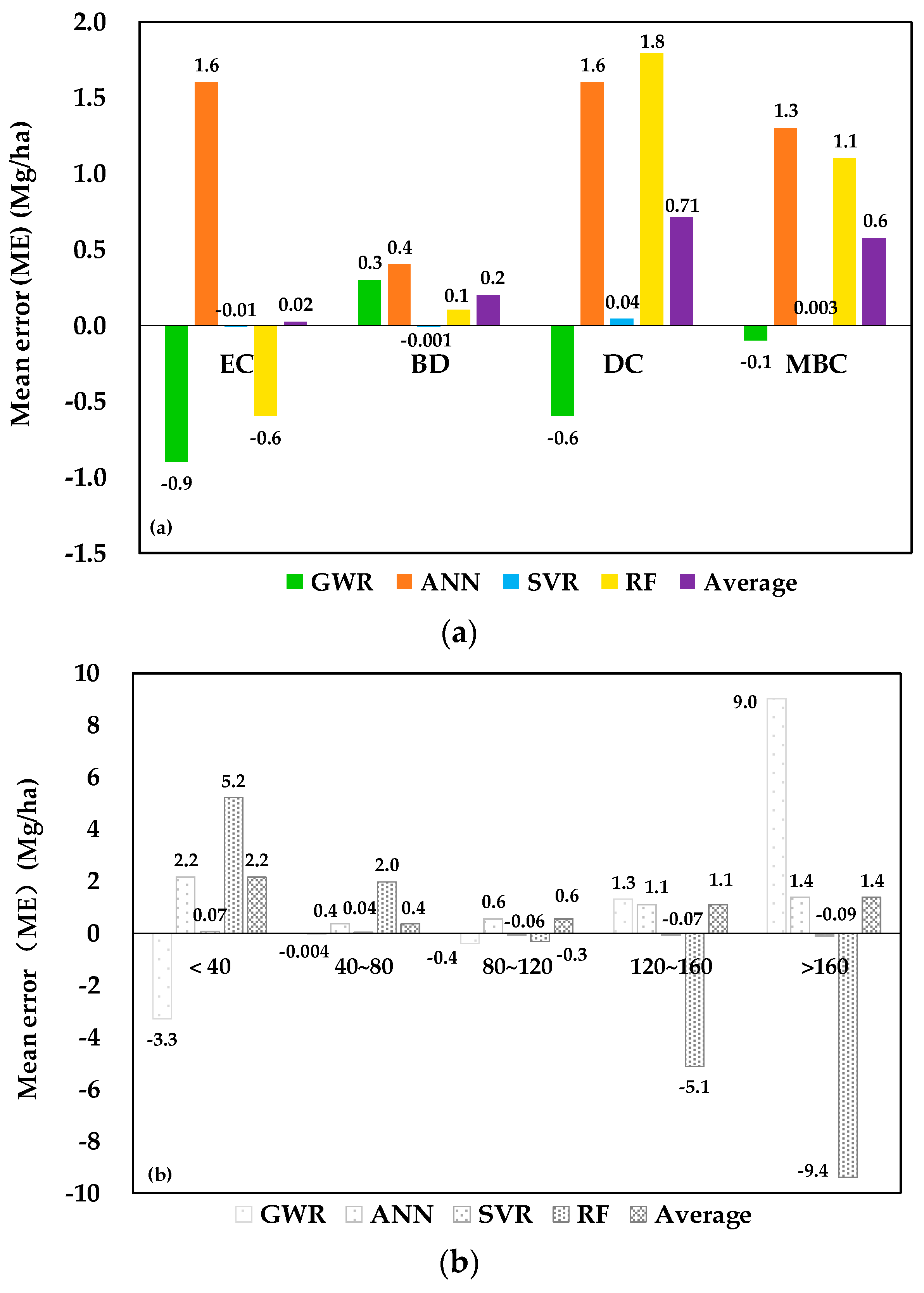
The mean errors of AGB prediction using the four models for different forest types and the measured values of AGB were also calculated to analyze the prediction accuracy of each forest type, and the data saturation in the Sentinel data was discussed (Figure 7). Generally, the estimated AGB values of the four forest types of 56 quadrats by the four models were all higher than the measured values (Figure 7a). Among that, the AGB estimation of the deciduous coniferous forests obtained the maximum error of 0.7 Mg·ha−1, and all models, excluding the GWR with ME values of −0.6 Mg·ha−1, performed the worst for deciduous coniferous forests compared to the other three forest types, with ME values ranging from 0.04 (SVR) to 1.8 (RF) Mg·ha−1. The AGB estimation of mixed broadleaf-conifer forests had the second-large error, with 0.6 Mg·ha−1, followed by that of broadleaved deciduous forests (0.2 Mg·ha−1) and evergreen coniferous forests (0.02 Mg·ha−1). As for the four models, the GWR performed best in the AGB estimation of mixed broadleaf-conifer forests, and the worst for evergreen coniferous forests. The ANN, SVR, and RF all gave the most accurate assessments for broadleaved deciduous forests. The ANN showed the least precise assessments for evergreen coniferous forests, but SVR and RF gave the worst for deciduous coniferous forests. In a word, the AGB estimation of broadleaved deciduous forests was the most accurate and stable in the study area using the four models based on Sentinel imagery. Among the five levels of AGB values, the last level with AGB above 160 Mg·ha−1 (from 160 to 320 Mg·ha−1) had the least accuracy and the most fluctuated errors, based on Sentinel imagery, while AGB from 40 to 120 Mg·ha−1 obtained relatively higher accuracies (Figure 7b). The saturation level shown in this study was much higher than other studies (at around 60–70 Mg·ha−1), using SAR C band data [102]. This could be attributed to the integration of abundant predictors from Sentinel-1 and Sentinel-2 in the study area with normal forest coverage, which was human-dominated zones with nearby towns and villages.
6. Conclusions
To map the distribution of forest AGB at a regional scale, Sentinel SAR and multispectral imagery were selected for a group of field quadrats with a resolution of 10 m. Four AGB models, one GWR model, and three ML models were built using these field measurements and remote-sensing datasets. The results demonstrated that SVR with SMO algorithms are the best for spatially predicting and mapping the patterns of AGB in the study site. The results also showed that the texture characteristics of Sentinel-1 and the vegetation biophysical variables of Sentinel-2 were the most relative and important predictors for explaining the observed variability of AGB in the area, and that the contributions of the other Sentinel-derived factors were only marginal. The AGB estimation of broadleaved deciduous forests was the most accurate, while the AGB above 160 Mg·ha−1 had the least accuracy, indicating data saturation of Sentinel imagery. Overall, the performance of the models in this study will inform the selection of predictive mapping techniques for forest AGB modeling, while the map that is generated will be instrumental for formulating spatially-targeted climate change mitigation and sustainable land management strategies. In the future, the model performance will be improved by incorporating other important environmental data (e.g., distance to the city center and roads, as well as human disturbance) and other up-to-date remote sensing techniques (e.g., Tandem-X and LiDAR), as well as the stochastic component of AGB.
Although SAR C band and optical multispectral techniques have few advantages for detecting the sensibility of forest AGB compared to SAR P band or LiDAR, the available free Sentinel series at a relatively high spatial resolution with full coverage is indeed useful information for applications in global forest AGB estimation. The study demonstrated encouraging results in forest AGB mapping of the normal vegetated area using Sentinel imagery; thus, it is helpful and valuable for vital information mining from the Sentinel series when it is applied to global forest AGB estimation.
Author Contributions
L.C., C.R., and B.Z. designed this research. L.C. and Y.X. conducted field sampling and performed the experiments. L.C. conducted the analysis and wrote the paper. C.R., B.Z., and Z.W. drafted the paper and revised it critically. All authors reviewed the manuscript.
Funding
This study was supported by the National Key Research and Development Project of China (No. 2016YFC0500300).
Acknowledgments
The authors are grateful to the ESA (https://scihub.copernicus.eu/) and USGS (http://glovis.usgs.gov/) for providing the Sentinel imagery and SRTM DEM.
Conflicts of Interest
The authors declare no conflict of interest.
References
- Olson, J.S.; Watts, J.; Allison, L.J. Carbon in Live Vegetation of Major World Ecosystems; Oak Ridge National Laboratory: Oak Ridge, TN, USA, 1983.
- Liu, K.; Wang, J.D.; Zeng, W.S.; Song, J.L. Comparison and evaluation of three methods for estimating forest above ground biomass using TM and GLAS data. Remote Sens. 2017, 9, 341. [Google Scholar] [CrossRef]
- Cairns, M.A.; Brown, S.; Helmer, E.H.; Baumgardner, G.A. Root biomass allocation in the world’s upland forests. Oecologia 1997, 111, 1–11. [Google Scholar] [CrossRef] [PubMed]
- Brown, S.; Schroeder, P.; Birdsey, R. Aboveground biomass distribution of US eastern hardwood forests and the use of large trees as an indicator of forest development. For. Ecol. Manag. 1997, 96, 37–47. [Google Scholar] [CrossRef]
- Deb, D.; Singh, J.P.; Deb, S.; Datta, D.; Ghosh, A.; Chaurasia, R.S. An alternative approach for estimating above ground biomass using Resourcesat-2 satellite data and artificial neural network in Bundelkhand region of India. Environ. Monit. Assess. 2017, 189, 576. [Google Scholar] [CrossRef] [PubMed]
- Kaasalainen, S.; Holopainen, M.; Karjalainen, M.; Vastaranta, M.; Kankare, V.; Karila, K.; Osmanoglu, B. Combining Lidar and Synthetic Aperture Radar data to estimate forest biomass: Status and prospects. Forests 2015, 6, 252–270. [Google Scholar] [CrossRef]
- Pan, Y.; Birdsey, R.A.; Fang, J.; Houghton, R.; Kauppi, P.E.; Kurz, W.A.; Phillips, O.L.; Shvidenko, A.; Lewis, S.L.; Canadell, J.G.; et al. A large and persistent carbon sink in the world’s forests. Science 2011, 333, 988–993. [Google Scholar] [CrossRef] [PubMed]
- Saatchi, S.S.; Harris, N.L.; Brown, S.; Lefsky, M.; Mitchard, E.T.A.; Salas, W.; Zutta, B.R.; Buermann, W.; Lewis, S.L.; Hagen, S.; et al. Benchmark map of forest carbon stocks in tropical regions across three continents. Proc. Natl. Acad. Sci. USA 2011, 108, 9899–9904. [Google Scholar] [CrossRef] [PubMed] [Green Version]
- Deo, R.K.; Russell, M.B.; Domke, G.M.; Andersen, H.E.; Cohen, W.B.; Woodall, C.W. Evaluating site-specific and generic spatial models of aboveground forest biomass based on Landsat time-series and LiDAR strip samples in the Eastern USA. Remote Sens. 2017, 9, 598. [Google Scholar] [CrossRef]
- Ene, L.T.; Naesset, E.; Gobakken, T.; Gregoire, T.G.; Stahl, G.; Holm, S. A simulation approach for accuracy assessment of two-phase post-stratified estimation in large-area LiDAR biomass surveys. Remote Sens. Environ. 2013, 133, 210–224. [Google Scholar] [CrossRef]
- Wu, C.F.; Shen, H.H.; Shen, A.H.; Deng, J.S.; Gan, M.Y.; Zhu, J.X.; Xu, H.W.; Wang, K. Comparison of machine-learning methods for above-ground biomass estimation based on Landsat imagery. J. Appl. Remote Sens. 2016, 10, 035010. [Google Scholar] [CrossRef]
- McRoberts, R.E.; Næsset, E.; Gobakken, T. Inference for lidar-assisted estimation of forest growing stock volume. Remote Sens. Environ. 2013, 128, 268–275. [Google Scholar] [CrossRef]
- Zhao, P.P.; Lu, D.S.; Wang, G.X.; Liu, L.J.; Li, D.Q.; Zhu, J.R.; Yu, S.Q. Forest aboveground biomass estimation in Zhejiang Province using the integration of Landsat TM and ALOS PALSAR data. Int. J. Appl. Earth Obs. 2016, 53, 1–15. [Google Scholar] [CrossRef]
- Kumar, L.; Sinha, P.; Taylor, S.; Alqurashi, A.F. Review of the use of remote sensing for biomass estimation to support renewable energy generation. J. Appl. Remote Sens. 2015, 9, 097696. [Google Scholar] [CrossRef]
- Lin, Y.; West, G. Reflecting conifer phenology using mobile terrestrial LiDAR: A case study of Pinus sylvestris growing under the Mediterranean climate in Perth, Australia. Ecol. Indic. 2016, 70, 1–9. [Google Scholar] [CrossRef]
- Blackard, J.A.; Finco, M.V.; Helmer, E.H.; Holden, G.R.; Hoppus, M.L.; Jacobs, D.M.; Lister, A.J.; Moisen, G.G.; Nelson, M.D.; Riemann, R.; et al. Mapping us forest biomass using nationwide forest inventory data and moderate resolution information. Remote Sens. Environ. 2008, 112, 1658–1677. [Google Scholar] [CrossRef]
- Cao, L.D.; Pan, J.J.; Li, R.J.; Li, J.L.; Li, Z.F. Integrating airborne LiDAR and optical data to estimate forest aboveground biomass in arid and semi-arid regions of China. Remote Sens. 2018, 10, 532. [Google Scholar] [CrossRef]
- Thenkabail, P.S.; Stucky, N.; Griscom, B.W.; Ashton, M.S.; Diels, J.; van der Meer, B.; Enclona, E. Biomass estimations and carbon stock calculations in the oil palm plantations of African derived savannas using IKONOS data. Int. J. Remote Sens. 2004, 25, 5447–5472. [Google Scholar] [CrossRef]
- Sun, G.; Ni, W.; Zhang, Z.; Xiong, C. Forest Aboveground Biomass Mapping using Spaceborne Stereo Imagery Acquired by Chinese ZY-3. In Proceedings of the AGU Fall Meeting, San Francisco, CA, USA, 14–18 December 2015; Volume 12, p. 2089. [Google Scholar]
- Kumar, L.; Mutanga, O. Remote sensing of above-ground biomass. Remote Sens. 2017, 9, 935. [Google Scholar] [CrossRef]
- Avitabile, V.; Baccini, A.; Friedl, M.A.; Schmullius, C. Capabilities and limitations of Landsat and land cover data for aboveground woody biomass estimation of Uganda. Remote Sens. Environ. 2012, 117, 366–380. [Google Scholar] [CrossRef]
- Santi, E.; Paloscia, S.; Pettinato, S.; Fontanelli, G.; Mura, M.; Zolli, C.; Maselli, F.; Chiesi, M.; Bottai, L.; Chirici, G. The potential of multifrequency SAR images for estimating forest biomass in Mediterranean areas. Remote Sens. Environ. 2017, 200, 63–73. [Google Scholar] [CrossRef]
- Laurin, G.V.; Chen, Q.; Lindsell, J.A.; Coomes, D.A.; Del Frate, F.; Guerriero, L.; Pirotti, F.; Valentini, R. Above ground biomass estimation in an African tropical forest with LiDAR and hyperspectral data. ISPRS J. Photogramm. Remote Sens. 2014, 89, 49–58. [Google Scholar] [CrossRef]
- Chi, H.; Sun, G.Q.; Huang, J.L.; Guo, Z.F.; Ni, W.J.; Fu, A.M. National forest aboveground biomass mapping from ICESat/GLAS data and MODIS imagery in China. Remote Sens. 2015, 7, 5534–5564. [Google Scholar] [CrossRef]
- Guo, Q.H.; Liu, J.; Tao, S.L.; Xue, B.L.; Li, L.; Xu, G.C.; Li, W.K.; Wu, F.F.; Li, Y.M.; Chen, L.H.; et al. Perspectives and prospects of LiDAR in forest ecosystem monitoring and modeling. Chin. Sci. Bull. 2014, 59, 459–478. [Google Scholar] [CrossRef]
- Wilkes, P.; Disney, M.; Vicari, M.B.; Calders, K.; Burt, A. Estimating urban above ground biomass with multi-scale LiDAR. Carbon Balance Manag. 2018, 13, 10. [Google Scholar] [CrossRef] [PubMed]
- Malenovsky, Z.; Rott, H.; Cihlar, J.; Schaepman, M.E.; Garcia-Santos, G.; Fernandes, R.; Berger, M. Sentinels for science: Potential of Sentinel-1, -2, and -3 missions for scientific observations of ocean, cryosphere, and land. Remote Sens. Environ. 2012, 120, 91–101. [Google Scholar] [CrossRef]
- Torres, R.; Snoeij, P.; Geudtner, D.; Bibby, D.; Davidson, M.; Attema, E.; Potin, P.; Rommen, B.; Floury, N.; Brown, M.; et al. GMES Sentinel-1 mission. Remote Sens. Environ. 2012, 120, 9–24. [Google Scholar] [CrossRef]
- Chang, J.S.; Shoshany, M. Mediterranean Shrublands Biomass Estimation using Sentinel-1 and Sentinel-2. In Proceedings of the 36th IEEE International Geoscience and Remote Sensing Symposium (IGARSS), Beijing, China, 10–15 July 2016; pp. 5300–5303. [Google Scholar]
- Laurin, G.V.; Puletti, N.; Hawthorne, W.; Liesenberg, V.; Corona, P.; Papale, D.; Chen, Q.; Valentini, R. Discrimination of tropical forest types, dominant species, and mapping of functional guilds by hyperspectral and simulated multispectral Sentinel-2 data. Remote Sens. Environ. 2016, 176, 163–176. [Google Scholar] [CrossRef] [Green Version]
- Liu, Y.A.; Gong, W.S.; Hu, X.Y.; Gong, J.Y. Forest type identification with random forest using Sentinel-1A, Sentinel-2A, multi-temporal Landsat-8 and DEM data. Remote Sens. 2018, 10, 946. [Google Scholar] [CrossRef]
- Tesfamichael, S.G.; Newete, S.W.; Adam, E.; Dubula, B. Field spectroradiometer and simulated multispectral bands for discriminating invasive species from morphologically similar cohabitant plants. GISci. Remote Sens. 2018, 55, 417–436. [Google Scholar] [CrossRef]
- Battude, M.; Al Bitar, A.; Morin, D.; Cros, J.; Huc, M.; Sicre, C.M.; Le Dantec, V.; Demarez, V. Estimating maize biomass and yield over large areas using high spatial and temporal resolution Sentinel-2 like remote sensing data. Remote Sens. 2016, 184, 668–681. [Google Scholar] [CrossRef]
- Su, W.; Hou, N.; Li, Q.; Zhang, M.Z.; Zhao, X.F.; Jiang, K.P. Retrieving leaf area index of corn canopy based on Sentinel-2 remote sensing image. Trans. Chin. Soc. Agric. Mach. 2018, 49, 151–156. [Google Scholar]
- Sanches, I.D.; Feitosa, R.Q.; Diaz, P.M.A.; Soares, M.D.; Luiz, A.J.B.; Schultz, B.; Maurano, L.E.P. Campo verde database: Seeking to improve agricultural remote sensing of tropical areas. IEEE Geosci. Remote Sens. Lett. 2018, 15, 369–373. [Google Scholar] [CrossRef]
- Sibanda, M.; Mutanga, O.; Rouget, M. Examining the potential of Sentinel-2 MSI spectral resolution in quantifying above ground biomass across different fertilizer treatments. ISPRS J. Photogramm. 2015, 110, 55–65. [Google Scholar] [CrossRef]
- Sakowska, K.; Juszczak, R.; Gianelle, D. Remote sensing of grassland biophysical parameters in the context of the Sentinel-2 satellite mission. J. Sens. 2016, 2016, 4612809. [Google Scholar] [CrossRef]
- Ali, I.; Cawkwell, F.; Dwyer, E.; Green, S. Modeling managed grassland biomass estimation by using multitemporal remote sensing data-A machine learning approach. IEEE J. Sel. Top. Appl. Earth Obs. Remote Sens. 2017, 10, 3254–3264. [Google Scholar] [CrossRef]
- Hawrylo, P.; Wezyk, P. Predicting growing stock volume of scots pine stands using Sentinel-2 satellite imagery and airborne image-derived point clouds. Forests 2018, 9, 274. [Google Scholar] [CrossRef]
- Mura, M.; Bottalico, F.; Giannetti, F.; Bertani, R.; Giannini, R.; Mancini, M.; Orlandini, S.; Travaglini, D.; Chirici, G. Exploiting the capabilities of the Sentinel-2 multi spectral instrument for predicting growing stock volume in forest ecosystems. Int. J. Appl. Earth Obs. 2018, 66, 126–134. [Google Scholar] [CrossRef]
- Plank, S. Rapid damage assessment by means of multi-temporal SAR-A comprehensive review and outlook to Sentinel-1. Remote Sens. 2014, 6, 4870–4906. [Google Scholar] [CrossRef] [Green Version]
- Chemura, A.; Mutanga, O.; Dube, T. Separability of coffee leaf rust infection levels with machine learning methods at Sentinel-2 MSI spectral resolutions. Precis. Agric. 2017, 18, 859–881. [Google Scholar] [CrossRef]
- Mallinis, G.; Mitsopoulos, I.; Chrysafi, I. Evaluating and comparing Sentinel 2A and Landsat-8 Operational Land Imager (OLI) spectral indices for estimating fire severity in a Mediterranean pine ecosystem of Greece. GISci. Remote Sens. 2018, 55, 1–18. [Google Scholar] [CrossRef]
- Baccini, A.; Goetz, S.J.; Walker, W.S.; Laporte, N.T.; Sun, M.; Sulla-Menashe, D.; Hackler, J.; Beck, P.S.A.; Dubayah, R.; Friedl, M.A.; et al. Estimated carbon dioxide emissions from tropical deforestation improved by carbon-density maps. Nat. Clim. Chang. 2012, 2, 182–185. [Google Scholar] [CrossRef]
- Lu, D. The potential and challenge of remote sensing–based biomass estimation. Int. J. Remote Sens. 2006, 27, 1297–1328. [Google Scholar] [CrossRef]
- Fassnacht, F.E.; Hartig, F.; Latifi, H.; Berger, C.; Hernandez, J.; Corvalan, P.; Koch, B. Importance of sample size, data type and prediction method for remote sensing-based estimations of aboveground forest biomass. Remote Sens. Environ. 2014, 154, 102–114. [Google Scholar] [CrossRef]
- Fotheringham, A.S.; Brunsdon, C.; Charlton, M.E. Geographically Weighted Regression: The Analysis of Spatially Varying Relationships; Wiley: Chichester, UK, 2002. [Google Scholar]
- Propastin, P. Modifying geographically weighted regression for estimating aboveground biomass in tropical rainforests by multispectral remote sensing data. Int. J. Appl. Earth Obs. 2012, 18, 82–90. [Google Scholar] [CrossRef]
- Gao, Y.K.; Lu, D.S.; Li, G.Y.; Wang, G.X.; Chen, Q.; Liu, L.J.; Li, D.Q. Comparative analysis of modeling algorithms for forest aboveground biomass estimation in a subtropical region. Remote Sens. 2018, 10, 627. [Google Scholar] [CrossRef]
- Gao, Y.; Bian, J.M.; Song, C. Study on the dynamic relation between spring discharge and precipitation in Fusong County, Changbai Mountain, Jilin Province of China. Water Sci. Technol. Water Supply 2016, 16, 428–437. [Google Scholar] [CrossRef]
- Yang, F.; Yao, Z.F.; Sun, J.L.; Zhu, Y.Q.; Wang, Z.M. The landscape pattern changes analysis of Changbai Mountain forest based on RS and GIS—A case study in Fusong and Antu Counties. Syst. Sci. Compr. Stud. Agric. 2010, 26, 431–437. (In Chinese) [Google Scholar]
- Chen, L.; Ren, C.Y.; Zhang, B.; Wang, Z.M.; Liu, M.Y. Quantifying urban land sprawl and its driving forces in Northeast China from 1990 to 2015. Sustainability 2018, 10, 188. [Google Scholar] [CrossRef]
- Li, X.N.; Guo, Q.X.; Wang, X.C.; Zheng, H.F. Allometry of understory tree species in a natural secondary forest in Northeast China. Sci. Silvae Sin. 2010, 46, 22–32. (In Chinese) [Google Scholar]
- Tang, X.G. Estimation of Forest Aboveground Biomass by Integrating ICESat/GLAS Waveform and TM Data. Ph.D. Thesis, University of Chinese Academy of Sciences, Beijing, China, 2013. (In Chinese). [Google Scholar]
- Castillo, J.A.A.; Apan, A.A.; Maraseni, T.N.; Salmo, S.G. Estimation and mapping of above-ground biomass of mangrove forests and their replacement land uses in the Philippines using Sentinel imagery. ISPRS J. Photogramm. Remote Sens. 2017, 134, 70–85. [Google Scholar] [CrossRef]
- Veci, L. Sentinel-1 Toolbox: SAR Basics Tutorial; ARRAY Systems Computing, Inc. and European Space Agency: Paris, France, 2015. [Google Scholar]
- Liu, C. Analysis of Sentinel-1 SAR Data for Mapping Standing Water in the Twente Region. Master’s Thesis, University of Twente, Enschede, The Netherlands, 2016. [Google Scholar]
- Pan, L.; Sun, Y.J. Estimation of Cunninghamia lanceolata forest biomass based on Sentinel-1 image texture information. J. Northeast For. Univ. 2018, 46, 58–62. (In Chinese) [Google Scholar]
- Jacquemoud, S.; Verhoef, W.; Baret, F.; Bacour, C.; Zarco-Tejada, P.J.; Asner, G.P.; François, C.; Ustin, S.L. PROSPECT + SAIL models: A review of use for vegetation characterization. Remote Sens. Environ. 2009, 113, S56–S66. [Google Scholar] [CrossRef]
- Haralick, R.M.; Shanmugam, K.; Denstien, I. Textural features for image classification. IEEE Trans. Syst. Man Cybern. 1973, 3, 610–621. [Google Scholar] [CrossRef]
- Rouse, J.W.; Haas, R.H.; Schell, J.A.; Deering, D.W. Monitoring Vegetation Systems in the Great Plains with ERTS. In Proceedings of the Third Earth Resources Technology Satellite-1 Symposium, Washington, DC, USA, 10–14 December 1973; Volume 1, pp. 309–317. [Google Scholar]
- Delegido, J.; Verrelst, J.; Alonso, L.; Moreno, J. Evaluation of Sentinel-2 red-edge bands for empirical estimation of green LAI and chlorophyll content. Sensors 2011, 11, 7063–7081. [Google Scholar] [CrossRef] [PubMed]
- Clevers, J.G.P.W.; De Jong, S.M.; Epema, G.F.; Van der Meer, F.D.; Bakker, W.H.; Skidmore, A.K.; Scholte, K.H. Derivation of the red edge index using the MERIS standard band setting. Int. J. Remote Sens. 2002, 23, 3169–3184. [Google Scholar] [CrossRef]
- Deering, D.W.; Rouse, J.W.; Haas, R.H.; Schell, J.A. Measuring Forage Production of Grazing Units from Landsat MSS data. In Proceedings of the Tenth International Symposium on Remote Sensing of Environment, Ann Arbor, MI, USA, 6 October 1975; Volume 2, pp. 1169–1178. [Google Scholar]
- O’brien, R.M. A caution regarding rules of thumb for variance inflation factors. Qual. Quant. 2007, 41, 673–690. [Google Scholar] [CrossRef]
- Were, K.; Bui, D.T.; Dick, Ø.B.; Singh, B.R. A comparative assessment of support vector regression, artificial neural networks, and random forests for predicting and mapping soil organic carbon stocks across an Afromontane landscape. Ecol. Indic. 2015, 52, 394–403. [Google Scholar] [CrossRef]
- Cheadle, C.; Vawter, M.P.; Freed, W.J.; Becker, K.G. Analysis of microarray data using Z score transformation. J. Mol. Diagn. 2003, 5, 73–81. [Google Scholar] [CrossRef]
- Brunsdon, C.; Fotheringham, S.; Charlton, M. Geographically Weighted Regression–Modelling Spatial Non-stationarity. In Workshop on Local Indicators of Spatial Association; University of Leicester: Leicester, UK, 1998; Volume 47, pp. 431–443. [Google Scholar]
- Kumar, S.; Lal, R.; Liu, D. A geographically weighted regression kriging approach for mapping soil organic carbon stock. Geoderma 2012, 189, 627–634. [Google Scholar] [CrossRef]
- Shin, J.; Temesgen, H.; Strunk, J.L.; Hilker, T. Comparing modeling methods for predicting forest attributes using LiDAR metrics and ground measurements. Can. J. Remote Sens. 2016, 42, 739–765. [Google Scholar] [CrossRef]
- Zhang, C.S.; Tang, Y.; Xu, X.L.; Kiely, G. Towards spatial geochemical modelling: Use of geographically weighted regression for mapping soil organic carbon contents in Ireland. Appl. Geochem. 2011, 26, 1239–1248. [Google Scholar] [CrossRef]
- Peter, M. Efficient statistical classification of satellite measurements. Int. J. Remote Sens. 2011, 32, 6109–6132. [Google Scholar] [Green Version]
- Ahmed, M.A.A.; Abd-Elrahman, A.; Escobedo, F.J.; Cropper, W.P.; Martin, T.A.; Timilsina, N. Spatially-explicit modeling of multi-scale drivers of aboveground forest biomass and water yield in watersheds of the Southeastern United States. J. Environ. Manag. 2017, 199, 158–171. [Google Scholar] [CrossRef] [PubMed]
- Nakaya, T.; Charlton, M.; Lewis, P.; Brunsdon, C.; Yao, J.; Fotheringham, S. GWR4 User Manual, Windows Application for Geographically Weighted Regression Modelling; Ritsumeikan University: Kyoto, Japan, 2014. [Google Scholar]
- Haykin, S.S. Neural Networks: A Comprehensive Foundation; Tsinghua University Press: Beijing, China, 2001. [Google Scholar]
- Zhu, Y.H.; Liu, K.; Liu, L.; Wang, S.G.; Liu, H.X. Retrieval of mangrove aboveground biomass at the individual species level with WorldView-2 images. Remote Sens. 2015, 7, 12192–12214. [Google Scholar] [CrossRef]
- Hornik, K. Multilayer feed forward network are universal approximators. Neural Netw. 1989, 2, 359–366. [Google Scholar] [CrossRef]
- Santi, E.; Paloscia, S.; Pettinato, S.; Chirici, G.; Mura, M.; Maselli, F. Application of Neural Networks for the retrieval of forest woody volume from SAR multifrequency data at L and C bands. Eur. J. Remote Sens. 2015, 48, 673–687. [Google Scholar] [CrossRef] [Green Version]
- Lee, S.; Evangelista, D.G. Earthquake-induced landslide susceptibility mapping using an artificial neural network. Nat. Hazards Earth Syst. Sci. 2006, 6, 687–695. [Google Scholar] [CrossRef]
- Ottoy, S.; De Vos, B.; Sindayihebura, A.; Hermy, M.; Van Orshoven, J. Assessing soil organic carbon stocks under current and potential forest cover using digital soil mapping and spatial generalisation. Ecol. Indic. 2017, 77, 139–150. [Google Scholar] [CrossRef]
- Vapnik, V.N. The Nature of Statistical Learning Theory. Statistics for Engineering and Information Science; Springer: New York, NY, USA, 2000. [Google Scholar]
- Li, M.; Im, J.; Quackenbush, L.J.; Liu, T. Forest biomass and carbon stock quantification using airborne LiDAR data: A case study over Huntington wildlife forest in the Adirondack Park. IEEE J. Sel. Top. Appl. Earth Obs. Remote Sens. 2014, 7, 3143–3156. [Google Scholar] [CrossRef]
- Meng, S.L.; Pang, Y.; Zhang, Z.J.; Jia, W.; Li, Z.Y. Mapping aboveground biomass using texture indices from aerial photos in a temperate forest of Northeastern China. Remote Sens. 2015, 7, 12192–12214. [Google Scholar] [CrossRef]
- Sharifi, A.; Amini, J.; Tateishi, R. Estimation of forest biomass using multivariate relevance vector regression. Photogramm. Eng. Remote Sens. 2016, 82, 41–49. [Google Scholar] [CrossRef]
- Platt, J. Fast Training of Support Vector Machines Using Sequential Minimal Optimization. In Advances in Kernel Methods–Support Vector Learning; MIT Press: Cambridge, MA, USA, 1999. [Google Scholar]
- Zeng, Z.; Hsieh, W.W.; Shabbar, A.; Burrows, W.R. Seasonal prediction of winter extreme precipitation over Canada by support vector regression. Hydrol. Earth Syst. Sci. 2011, 15, 65–74. [Google Scholar] [CrossRef] [Green Version]
- Singh, M.; Evans, D.; Friess, D.A.; Tan, B.S.; Nin, C.S. Mapping above-ground biomass in a tropical forest in Cambodia using canopy textures derived from Google Earth. Remote Sens. 2015, 7, 5057–5076. [Google Scholar] [CrossRef]
- Rabe, A.; van der Linden, S.; Hostert, P. Simplifying Support Vector Machines for Regression Analysis of Hyperspectral Imagery. In Proceedings of the 1st Workshop on Hyperspectral Image and Signal Processing–Evolution in Remote Sensing, Grenoble, France, 26–28 August 2009. [Google Scholar]
- Breiman, L. Random Forests. Mach. Learn. 2001, 45, 5–32. [Google Scholar] [CrossRef] [Green Version]
- Breiman, L. Bagging predictors. Mach. Learn. 1996, 24, 123–140. [Google Scholar] [CrossRef] [Green Version]
- Amit, Y.; Geman, D. Shape quantization and recognition with randomized trees. Neural Comput. 1997, 9, 1545–1588. [Google Scholar] [CrossRef]
- Dhanda, P.; Nandy, S.; Kushwaha, S.P.S.; Ghosh, S.; Murthy, Y.V.N.K.; Dadhwal, V.K. Optimizing spaceborne LiDAR and very high resolution optical sensor parameters for biomass estimation at ICESat/GLAS footprint level using regression algorithms. Prog. Phys. Geogr. 2017, 41, 247–267. [Google Scholar] [CrossRef]
- Genuer, R.; Poggi, J.-M.; Tuleau-Malot, C.; Villa-Vialaneix, N. Random forests for big data. Big Data Res. 2017, 9, 28–46. [Google Scholar] [CrossRef]
- Jovic, A.; Bogunovic, N. Electrocardiogram analysis using a combination of statistical, geometric, and nonlinear heart rate variability features. Artif. Intell. Med. 2011, 51, 175–186. [Google Scholar] [CrossRef] [PubMed]
- Mutanga, O.; Adam, E.; Cho, M.A. High density biomass estimation for wetland vegetation using WorldView-2 imagery and random forest regression algorithm. Int. J. Appl. Earth. Obs. 2012, 18, 399–406. [Google Scholar] [CrossRef]
- Isaaks, E.H.; Srivastava, R.M. An Introduction to Applied Geostatistics; Oxford University Press: Oxford, UK, 1989. [Google Scholar]
- Wang, D.L.; Xin, X.P.; Shao, Q.Q.; Brolly, M.; Zhu, Z.L.; Chen, J. Modeling aboveground biomass in Hulunber grassland ecosystem by using unmanned aerial vehicle discrete Lidar. Sensors 2017, 17, 180. [Google Scholar] [CrossRef] [PubMed]
- Bourgoin, C.; Blanc, L.; Bailly, J.S.; Cornu, G.; Berenguer, E.; Oszwald, J.; Tritsch, I.; Laurent, F.; Hasan, A.F.; Sist, P.; et al. The potential of multisource remote sensing for mapping the biomass of a degraded Amazonian forest. Forests 2018, 9, 303. [Google Scholar] [CrossRef]
- Ghosh, S.M.; Behera, M.D. Aboveground biomass estimation using multi-sensor data synergy and machine learning algorithms in a dense tropical forest. Appl. Geogr. 2018, 96, 29–40. [Google Scholar] [CrossRef]
- Berninger, A.; Lohberger, S.; Stangel, M.; Siegert, F. SAR-based estimation of above-ground biomass and its changes in tropical forests of Kalimantan using L- and C-band. Remote Sens. 2018, 10, 831. [Google Scholar] [CrossRef]
- Vafaei, S.; Soosani, J.; Adeli, K.; Fadaei, H.; Naghavi, H.; Pham, T.D.; Bui, D.T. Improving accuracy estimation of forest aboveground biomass based on incorporation of ALOS-2 PALSAR-2 and Sentinel-2A imagery and machine learning: A case study of the Hyrcanian forest area (Iran). Remote Sens. 2018, 10, 172. [Google Scholar] [CrossRef]
- Sinha, S.; Jeganathan, C.; Sharma, L.K. A review of radar remote sensing for biomass estimation. Int. J. Environ. Sci. Technol. 2015, 12, 1779–1792. [Google Scholar] [CrossRef] [Green Version]
Figure 1.
The location of the study area and surveyed forest quadrats.

Figure 2.
Flowchart of steps used for forest above-ground biomass mapping using Sentinel SAR and multispectral imagery. DBH is the abbreviation of diameter at breast height.
Figure 2.
Flowchart of steps used for forest above-ground biomass mapping using Sentinel SAR and multispectral imagery. DBH is the abbreviation of diameter at breast height.

Figure 3.
Schematic representation of an example multi-layer perception neural network (MLPNN) model structure to predict forest above-ground biomass. Shown are the inputs with their neurons oi, and interlinked connections from each input to all hidden layer neurons oj, along with the selected weightings. The weighted outputs were then merged and fed into the output neuron ok to form the output values.

Figure 4.
Training errors associated with a given number of neurons in the hidden layer.

Figure 5.
Scatterplots of the measured and estimated above-ground biomass (AGB, Mg·ha−1).

Figure 6.
Predicted maps of above-ground biomass in the study site derived from (a) geographically weighted regression (GWR), (b) multi-layer perception neural network (ANN), (c) support vector machines for regression (SVR), and (d) random forests (RF). YJ, YQ, LJ, LS, and ED are the abbreviations of Yanjiang, Yongqing, Liangjiang, Lushuihe, and Erdaobaihe towns, respectively.

Figure 7.
The mean errors of the above-ground biomass predictions for (a) different forest types, (b) different AGB using geographically weighted regression (GWR), the multi-layer perception neural network (ANN), support vector machines for regression (SVR), and random forests (RF). EC, BD, DC, and MBC represent evergreen coniferous, broadleaved deciduous, deciduous coniferous, and mixed broadleaf-conifer forests, respectively.


Table 1.
List of Sentinel imagery acquired for the study.
| Mission | Product | Observation Date | Cell Size (m) | Uniform Resource Identifier (URI) |
|---|---|---|---|---|
| Sentinel-1B | Level-1 GRD-HR | 22 September 2017 | 10 | S1B_IW_GRDH_1SDV_20170922T213003_20170922T213028_007510_00D425_4962.SAFE |
| Sentinel-2A | Multispectral image Level-1C | 3 May 2017 | 10 | S2A_MSIL1C_20170503T021611_N0205_R003_T52TDN_20170503T022350.SAFE |
| Sentinel-2A | Multispectral image Level-1C | 25 July 2017 | 10 | S2A_MSIL1C_20170725T022551_N0205_R046_T52TCM_20170725T023524.SAFE |
| Sentinel-2A | Multispectral image Level-1C | 23 September 2017 | 10 | S2A_MSIL1C_20170923T022551_N0205_R046_T52TCN_20170923T023519.SAFE |
| Sentinel-2A | Multispectral image Level-1C | 23 September 2017 | 10 | S2A_MSIL1C_20170923T022551_N0205_R046_T52TDM_20170923T023519.SAFE |
Table 2.
Main allometric equations for the above-ground biomass calculation of each tree species [53,54].
| Tree Species | Allometric Equations |
|---|---|
| Betula platyphylla Suk. | AGB = T + B + L = 0.04939 × (D2 × H)0.9011 + 0.01417 × (D2 × H)0.7686 + 0.0109 × (D2 × H)0.6472 |
| Acer mono Maxim. | AGB = T + B + L = 0.3274 × (D2 × H)0.7218 + 0.01349 × (D2 × H)0.7198 + 0.02347 × (D2 × H)0.6929 |
| Tilia amurensis Rupr. | AGB = T + B + L = 0.01275 × (D2 × H)1.0094 + 0.00182 × (D2 × H)0.9746 + 0.00024 × (D2 × H)0.9907 |
| Mongolian oak (Quercus spp.) | AGB = T + B + L = 0.03147 × (D2 × H)0.7329 + 0.002127 × D2.9504 + 0.00321 × D2.47349 |
| Ulmus japonica Sarg. | AGB = T + B + L = 0.031457 × (D2 × H)1.032 + 0.007429 × D2.6745 + 0.002754 × D2.4965 |
| Fraxinus mandschurica Rupr | AGB = T + B + L = 1.416 × D1.71 + 1.154 × D1.549 + 0.7655 × D0.886 |
| Populus cathayana Rehd. | AGB = T + B + L = 0.3642 × D2.0043 + 0.0317 × D2.6398 + 0.0149 × D2.2541 |
| Juglans mandshurica Maxim. | AGB = 0.099 × (D2H)0.841 |
| Prunus padus L. | AGB = 0.09 × D2.696 |
| Pinus koraiensis Sieb. et Zucc. | AGB = T + B + L = 0.0144 × (D2 × H)1.0004 + 0.0332 × (D2 × H)0.6941 + 0.0866 × (D2 × H)0.4696 |
| Larix gmelinii var. japonica | AGB = T + B + L = 0.025 × (D2 × H)0.96 + 0.0021 × (D2 × H)0.9638 + 0.00126 × (D2 × H)0.9675 |
AGB, T, B, L, D, and H represent above-ground biomass, tree trunk biomass, branch biomass, leaf biomass, diameter at breast height, and tree height, respectively.
Table 3.
Sentinel-based imagery data predictors of above-ground biomass.
| Source Image | Relevant Predictors | Description | |
|---|---|---|---|
| Sentinel-1 | Polarization | VV | vertical transmit-vertical channel |
| VH | vertical transmit-Horizontal channel | ||
| V/H 1 | VV/VH | ||
| Texture 2 | VH_CON, VV_CON | Contrast | |
| VH_DIS, VV_DIS | Dissimilarity | ||
| VH_HOM, VV_HOM | Homogeneity | ||
| VH_ASM, VV_ASM | Angular Second Moment | ||
| VH_ENE, VV_ENE | Energy | ||
| VH_MAX, VV_MAX | Maximum Probability | ||
| VH_ENT, VV_ENT | Entropy | ||
| VH_MEA, VV_MEA | GLCM Mean | ||
| VH_VAR, VV_VAR | GLCM Variance | ||
| VH_COR, VV_COR | GLCM Correlation | ||
| Sentinel-2 | Multispectral bands | B2 | Blue, 490 nm |
| B3 | Green, 560 nm | ||
| B4 | Red, 665 nm | ||
| B5 | Red edge, 705 nm | ||
| B6 | Red edge, 749 nm | ||
| B7 | Red edge, 783 nm | ||
| B8 | Near Infrared, 842 nm | ||
| B8a | Near Infrared, 865 nm | ||
| B11 | Short Wave IR, 1610 nm | ||
| B12 | Short Wave IR, 2190 nm | ||
| Vegetation indices | NDVI 3 | (Band 8 − Band 4)/(Band 8 + Band 4) | |
| NDI45 4 | (Band 5 − Band 4)/(Band 5 + Band 4) | ||
| IRECI 5 | (Band 7 − Band 4)/(Band 5/Band 6) | ||
| TNDVI 6 | [(Band 8 − Band 4)/(Band 8 + Band 4) + 0.5]1/2 | ||
| Vegetation biophysical variables | LAI | Leaf Area Index | |
| FVC | Fraction of Vegetation Cover | ||
| FPAR | Fraction of Absorbed Photosynthetically Active Radiation | ||
| Cab | Chlorophyll content in the leaf | ||
| SRTM DEM | Elevation | H | Elevation, 30 m resolution |
1 Pan and Sun (2018) [58]; 2 GLCM = Gray-level Co-occurrence Matrix with a nine by nine-pixel window, Haralick et al. (1973) [60]; 3 NDVI = Normalized Difference Vegetation Index, Rouse et al. (1973) [61]; 4 NDI45 = Normalized Difference Vegetation Index with band 4 and 5, Delegido et al. (2011) [62]; 5 IRECI = Inverted Red-Edge Chlorophyll Index, Clevers et al. (2002) [63]; 6 TNDVI = Transformed Normalised Difference Vegetation Index, Deering et al. (1975) [64].
Table 4.
Performance evaluation of the GWR, ANN, SVR, and RF models.
| Evaluation Index | GWR | ANN | SVR | RF |
|---|---|---|---|---|
| ME | 0.04 | 0.84 | 4 × 10⁻³ | 0.55 |
| MAE | 4.01 | 1.21 | 0.07 | 3.48 |
| RMSE | 5.26 | 1.73 | 0.08 | 4.43 |
| r | 0.995 | 1 | 1 | 0.999 |
ME, MAE, RMSE, and r are the abbreviations of mean error, mean absolute error, root mean squared error, and correlation coefficient, respectively. The p-values of r were all below 0.01.
© 2018 by the authors. Licensee MDPI, Basel, Switzerland. This article is an open access article distributed under the terms and conditions of the Creative Commons Attribution (CC BY) license (http://creativecommons.org/licenses/by/4.0/).
Share and Cite
MDPI and ACS Style
Chen, L.; Ren, C.; Zhang, B.; Wang, Z.; Xi, Y. Estimation of Forest Above-Ground Biomass by Geographically Weighted Regression and Machine Learning with Sentinel Imagery. Forests 2018, 9, 582. https://doi.org/10.3390/f9100582
AMA Style
Chen L, Ren C, Zhang B, Wang Z, Xi Y. Estimation of Forest Above-Ground Biomass by Geographically Weighted Regression and Machine Learning with Sentinel Imagery. Forests. 2018; 9(10):582. https://doi.org/10.3390/f9100582
Chicago/Turabian StyleChen, Lin, Chunying Ren, Bai Zhang, Zongming Wang, and Yanbiao Xi. 2018. "Estimation of Forest Above-Ground Biomass by Geographically Weighted Regression and Machine Learning with Sentinel Imagery" Forests 9, no. 10: 582. https://doi.org/10.3390/f9100582
Note that from the first issue of 2016, this journal uses article numbers instead of page numbers. See further details here.