Predicting Volume and Biomass Change from Multi-Temporal Lidar Sampling and Remeasured Field Inventory Data in Panther Creek Watershed, Oregon, USA

Abstract
:1. Introduction
2. Materials and Methods
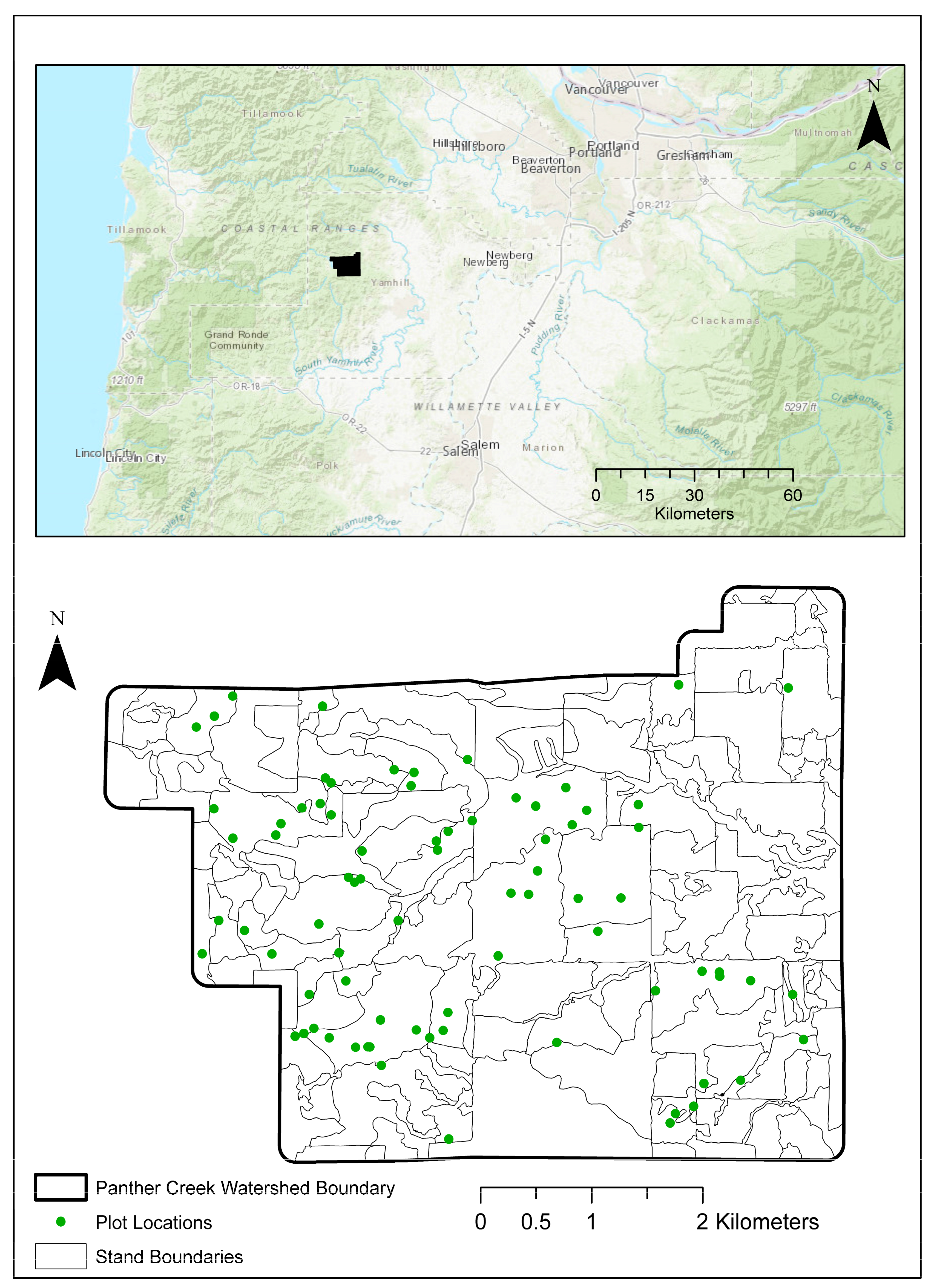
2.1. Study Area
2.2. Data
2.2.1. Ground Data
2.2.2. Lidar Data
- LCH4007 and LCH4012: 40th percentiles of all-returns lidar canopy height above 1 m in 2007 and 2012, respectively.
- LCH6007 and LCH6012: 60th percentiles of all-returns lidar canopy height above 1 m in 2007 and 2012, respectively.
- LCHV07 and LCHV12: variance of all-returns lidar data in 2007 and 2012.
- PCC07 and PCC12: percent of all-returns lidar heights, within each circular plot, above 1 m for the 2007 and 2012 data.
- ∆LCH40, ∆LCH60 and ∆PCC: differences in the 40th percentiles, 60th percentiles, and percent of all-returns lidar heights above 1 m between 2007 and 2012, respectively.
2.3. Statistical Analysis
3. Results and Discussion
4. Summary and Conclusions
Acknowledgments
Author Contributions
Conflicts of Interest
References
- Næsset, E. Predicting forest stand characteristics with airborne scanning laser using a practical two-stage procedure and field data. Remote Sens. Environ. 2002, 80, 88–99. [Google Scholar] [CrossRef]
- White, J.; Wulder, M.; Varhola, A.; Vastaranta, M.; Coops, N.; Cook, B.; Pitt, D.; Woods, M. A best practices guide for generating forest inventory attributes from airborne laser scanning data using an area-based approach. In Information Report FI-X-010; Natural Resources Canada, Canadian Forest Service, Pacific Forestry Centre: Victoria, BC, Canada, 2013; p. 50. [Google Scholar]
- Flewelling, J.W.; McFadden, G. LiDAR data and cooperative research at Panther Creek, Oregon. In Proceedings of the SilviLaser, Hobart, Austria, 16–20 October 2011. [Google Scholar]
- Temesgen, H.; Strunk, J.; Anderson, H.-E.; Flewelling, J. Evaluating different models to predict biomass increment from multi-temporal lidar sampling and remeasured field inventory data in South-central Alaska. Math. Comput. For. Nat. Res. Sci. 2015, 7, 66–80. [Google Scholar]
- Tonolli, S.; Dalponte, M.; Vescovo, L.; Rodeghiero, M.; Bruzzone, L.; Damiano, G. Mapping and modeling forest tree volume using forest inventory and airborne laser scanning. Eur. J. For. Res. 2010, 130, 1764–1772. [Google Scholar] [CrossRef]
- Goerndt, M.E.; Monleon, V.J.; Temesgen, H. A comparison of small-area estimation techniques to estimate selected stand attributes using LiDAR-derived auxiliary variables. Can. J. For. Res. 2011, 41, 1189–1201. [Google Scholar] [CrossRef]
- Chen, Q. Modeling aboveground tree woody biomass using national-scale allometric methods and airborne lidar. ISPRS J. Photogramm. Remote Sens. 2015, 106, 95–106. [Google Scholar] [CrossRef]
- Næsset, E.; Gobakken, T.; Holmgren, J.; Hyyppä, H.; Hyyppä, J.; Maltamo, M. Laser scanning of forest resources: The Nordic experience. Scand. J. For. Res. 2004, 19, 482–499. [Google Scholar] [CrossRef]
- Wulder, M.A.; White, J.C.; Fournier, R.A.; Luther, J.E.; Magnussen, S. Spatially explicit large area biomass estimation: Three approaches using forest inventory and remotely sensed imagery in a GIS. Sensors 2008, 8, 529–560. [Google Scholar] [CrossRef] [PubMed]
- Temesgen, H.; Affleck, D.; Poudel, K.; Gray, A.; Sessions, J. A review of the challenges and opportunities in estimating above ground forest biomass using tree-level models. Scand. J. For. Res. 2015, 30, 326–335. [Google Scholar] [CrossRef]
- Hudak, A.T.; Strand, E.K.; Vierling, L.A.; Byrne, J.C.; Eitel, J.U.H.; Martinuzzi, S.; Falkowski, M.J. Quantifying aboveground forest carbon pools and fluxes from repeat LiDAR surveys. Remote Sens. Environ. 2012, 123, 25–40. [Google Scholar] [CrossRef]
- Bollandsås, O.M.; Gregoire, T.; Næsset, E.; Øyen, B.H. Detection of biomass change in a Norwegian mountain forest area using small footprint airborne laser scanner data. Stat. Methods Appl. 2013, 22, 113–129. [Google Scholar] [CrossRef]
- Næsset, E.; Bollandsås, O.M.; Gobakken, T.; Gregoire, T.; Ståhl, G. Model-assisted estimation of change in forest biomass over an 11 year period in a sample survey supported by airborne LiDAR: A case study with post-stratification to provide “activity data”. Remote Sens. Environ. 2013, 128, 299–314. [Google Scholar] [CrossRef]
- Næsset, E.; Gobakken, T. Estimating forest growth using canopy metrics derived from airborne laser scanner data. Remote Sens. Environ. 2005, 96, 453–465. [Google Scholar] [CrossRef]
- Yu, X.; Hyyppä, J.; Kaartinen, H.; Maltamo, M.; Hyyppä, H. Obtaining plotwise mean height and volume growth in boreal forests using multi-temporal laser surveys and various change detection techniques. Int. J Remote Sens. 2008, 29, 1367–1386. [Google Scholar] [CrossRef]
- Nakajima, T.; Hirata, Y.; Hiroshima, T.; Furuya, N.; Tatsuhara, S.; Tsuyuki, S.; Shiraishi, N. A growth prediction system for local stand volume derived from lidar data. GISci. Remote Sens. 2011, 48, 394–415. [Google Scholar] [CrossRef]
- Nakajima, T. Estimating tree growth using crown metrics derived from lidar data. J. Indian Soc. Remote Sens. 2016, 44, 217–223. [Google Scholar] [CrossRef]
- Bailey, R.G. Description of the Ecoregions of the United States, 2nd ed.; USDA Forest Service: Washington, DC, USA, 1995; p. 108.
- Poudel, K.P.; Temesgen, H. Methods for estimating aboveground biomass and its components for Douglas-fir and lodgepole pine trees. Can. J. For. Res. 2016, 46, 77–87. [Google Scholar] [CrossRef]
- McGaughey, R.J. FUSION/LDV: Software for LIDAR Data Analysis and Visualization; USDA Forest Service, Pacific Northwest Research Station, University of Washington: Seattle, WA, USA, 2004.
- R Core Team. R: A Language and Environment for Statistical Computing. R Foundation for Statistical Computing, Vienna, Austria, 2017. Available online: https://www.R-project.org/ (accessed on 12 December 2017).
- Pinheiro, J.; Bates, D.; DebRoy, S.; Sarkar, D.; R Core Team. nlme: Linear and Nonlinear Mixed Effects Models. R Package Version 3.4.1. 2017. Available online: https://CRAN.R-project.org/package=nlme (accessed on 12 December 2017).
- Leys, C.; Christophe, L.; Klein, O.; Bernard, P.; Licata, L. Detecting outliers: Do not use standard deviation around the mean, use absolute deviation around the median. J. Exp. Soc. Psychol. 2013, 49, 764–766. [Google Scholar] [CrossRef]
- Efron, B.; Gong, G. A leisurely look at the bootstrap, the jackknife, and cross-validation. Am. Stat. 1983, 37, 36–48. [Google Scholar]
- Kearns, M.; Ron, D. Algorithmic stability and sanity-check bounds for leave-one-out cross-validation. Neural Comput. 1997, 11, 1427–1453. [Google Scholar] [CrossRef]
- Poudel, K.P.; Temesgen, H. Calibration of volume and component biomass equations for Douglas-fir and lodgepole pine in Western Oregon forests. For. Chron. 2016, 92, 172–182. [Google Scholar] [CrossRef]
- Temesgen, H.; Monleon, V.J.; Weiskittel, A.R.; Wilson, D.S. Sampling strategies for efficient estimation of tree foliage biomass. For. Sci. 2011, 57, 153–163. [Google Scholar]


| Variable | 2007 | 2012 | ||||||
|---|---|---|---|---|---|---|---|---|
| Min | Mean | Max | SD | Min | Mean | Max | SD | |
| DBH | 0.50 | 26.18 | 162.00 | 18.75 | 0.90 | 28.36 | 165.40 | 18.92 |
| HT | 1.40 | 21.28 | 63.40 | 12.05 | 0.20 | 22.91 | 63.10 | 12.08 |
| VPH | 3.51 | 575.49 | 1744.22 | 397.23 | 21.00 | 622.60 | 1836.80 | 401.48 |
| AGBPH | 8.97 | 302.06 | 828.81 | 175.17 | 37.97 | 321.02 | 851.86 | 174.50 |
| LCH40 | 1.03 | 16.79 | 37.16 | 9.37 | 1.52 | 19.76 | 39.56 | 8.86 |
| LCH60 | 1.93 | 22.22 | 41.80 | 10.22 | 2.31 | 24.78 | 43.10 | 9.54 |
| LCHV | 0.72 | 111.30 | 380.33 | 86.68 | 5.18 | 114.24 | 381.78 | 83.22 |
| PCC | 1.09 | 80.02 | 96.00 | 20.37 | 29.94 | 85.36 | 96.42 | 12.59 |
| Growth | ||||||||
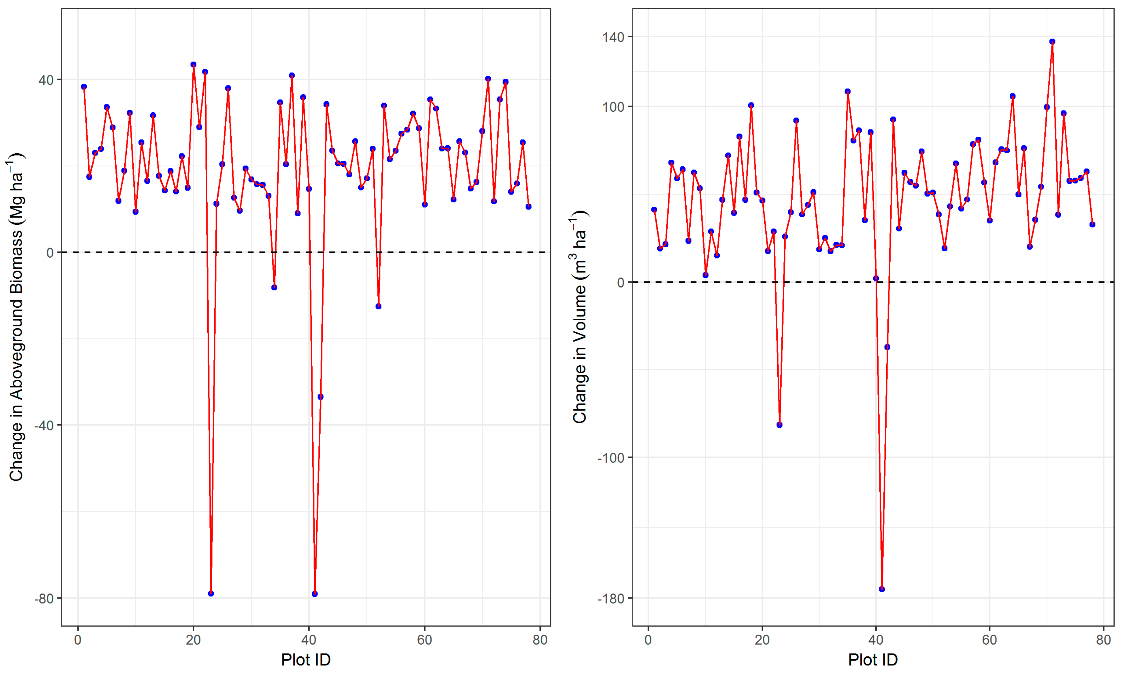
| VPH | −174.91 | 47.12 | 136.93 | 41.14 | ||||
| AGBPH | −79.04 | 18.96 | 43.51 | 20.12 | ||||
| LCH40 | −10.91 | 2.97 | 20.74 | 3.53 | ||||
| LCH60 | −4.46 | 2.56 | 6.03 | 1.55 | ||||
| PCC | −21.30 | 5.34 | 50.81 | 11.17 | ||||
| Approach | Model | Parameter (Standard Error) | R2 | ||
|---|---|---|---|---|---|
| A1 | 1.0 | −112.7205 (49.0673) | 1.4335 (0.1602) | 3.2519 (0.5995) | 0.64 |
| A1 | 1.1 | −206.7080 (84.4578) | 1.5970 (0.1660) | 4.1412 (0.9876) | 0.64 |
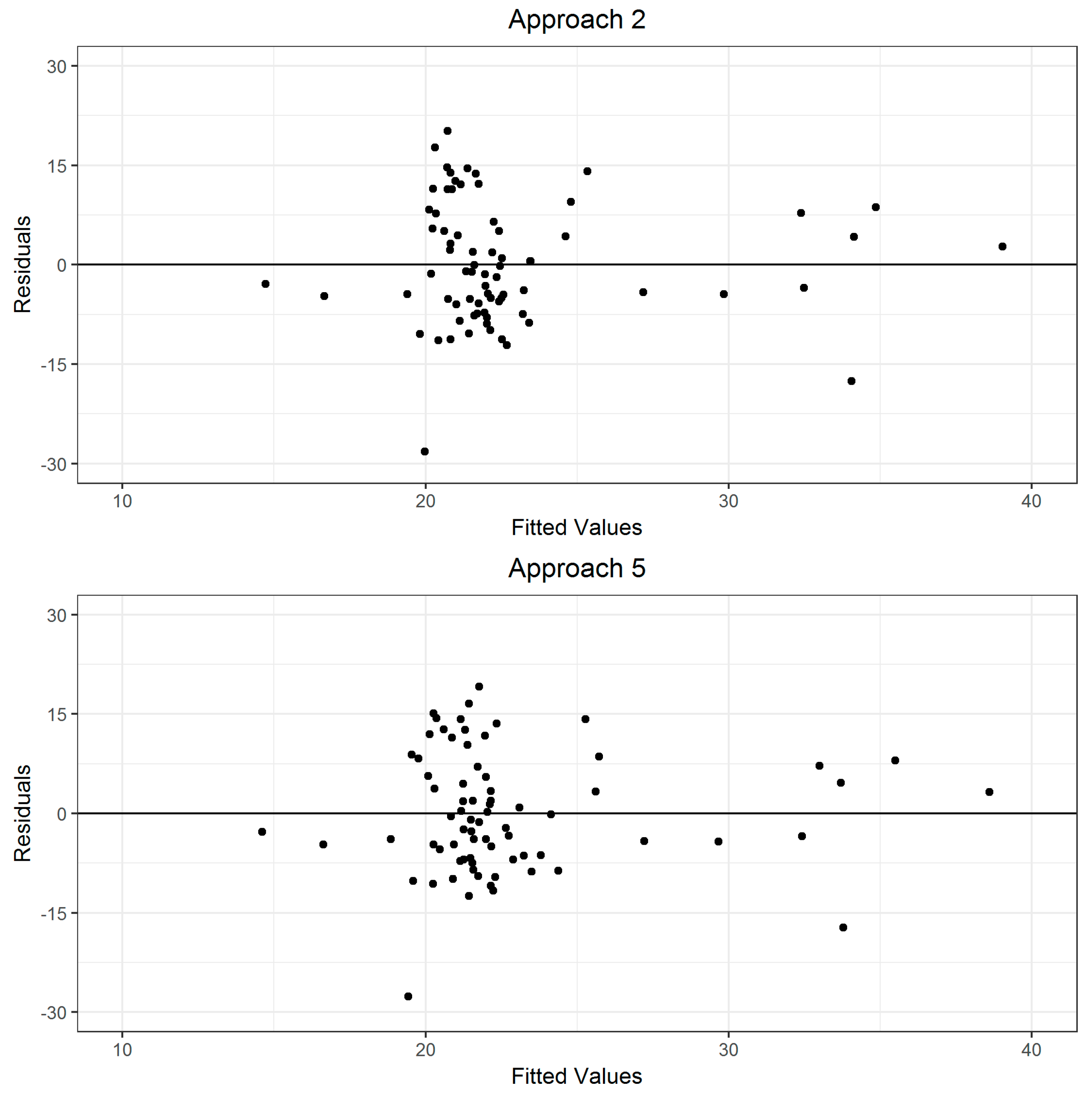
| A2 | 2 | 22.6334 (1.5774) | −0.6031 (0.3416) | 0.3535 (0.0990) | 0.17 |
| A3 | 3 | 20.4517 (1.3812) | 0.1008 (0.0366) | - | 0.10 |
| A4 | 4.0 | −71.6786 (68.8690) | 1.2609 (0.1942) | 3.1908 (0.7429) | 0.69 |
| A4 | 4.1 | −145.9440 (93.9257) | 1.4984 (0.1838) | 3.5907 (1.0721) | 0.66 |
| A5 | 5 | 23.0565 (1.8158) | −0.6644 (0.3471) | 0.3434 (0.1044) | 0.19 |
| A6 | 6 | 21.6315 (1.8878) | 0.0769 (0.0444) | - | 0.10 |
| Approach | Bias () | Bias Percent | RMSE () | RMSE Percent |
|---|---|---|---|---|
| A1 | −0.21 | −0.92 | 31.30 | 137.64 |
| A2 | −0.04 | −0.18 | 9.30 | 40.90 |
| A3 | 0.07 | 0.31 | 9.61 | 42.26 |
| A4 | −0.26 | −1.13 | 28.50 | 125.30 |
| A5 | −0.02 | −0.07 | 9.42 | 41.42 |
| A6 | 0.06 | 0.25 | 9.88 | 43.45 |
| Approach | Model | Parameter (Standard Error) | R2 | ||
|---|---|---|---|---|---|
| A1 | 1.0 | −269.1384 (102.4261) | 3.5070 (0.3069) | 5.7652 (1.2567) | 0.710 |
| A1 | 1.1 | −524.0004 (182.6992) | 3.6709 (0.3307) | 8.6432 (2.1417) | 0.684 |
| A2 | 2 | 33.1701 (6.8663) | 8.3630 (2.4188) | −0.6203 (0.2999) | 0.153 |
| A3 | 3 | 50.3331 (4.3807) | 0.0271 (0.0549) | - | 0.003 |
| A4 | 4.0 | −131.4910 (149.1598) | 3.0154 (0.4063) | 5.1304 (1.5635) | 0.756 |
| A4 | 4.1 | −148.2289 (233.4982) | 2.9270 (0.4686) | 5.4781 (2.4128) | 0.735 |
| A5 | 5 | 27.7979 (8.3186) | 8.1724 (2.4947) | −0.3344 (0.3395) | 0.221 |
| A6 | 6 | 39.5584 (7.5935) | 0.1225 (0.0854) | - | 0.151 |
| Approach | Bias () | Bias Percent | RMSE () | RMSE Percent |
|---|---|---|---|---|
| A1 | −0.60 | −1.16 | 72.16 | 139.47 |
| A2 | −0.13 | −0.26 | 28.12 | 54.36 |
| A3 | −0.33 | −0.63 | 29.55 | 57.12 |
| A4 | 0.06 | 0.11 | 51.56 | 99.65 |
| A5 | −0.07 | −0.13 | 28.44 | 54.97 |
| A6 | −0.21 | −0.40 | 28.75 | 55.58 |
© 2018 by the authors. Licensee MDPI, Basel, Switzerland. This article is an open access article distributed under the terms and conditions of the Creative Commons Attribution (CC BY) license (http://creativecommons.org/licenses/by/4.0/).
Share and Cite
Poudel, K.P.; Flewelling, J.W.; Temesgen, H. Predicting Volume and Biomass Change from Multi-Temporal Lidar Sampling and Remeasured Field Inventory Data in Panther Creek Watershed, Oregon, USA. Forests 2018, 9, 28. https://doi.org/10.3390/f9010028
Poudel KP, Flewelling JW, Temesgen H. Predicting Volume and Biomass Change from Multi-Temporal Lidar Sampling and Remeasured Field Inventory Data in Panther Creek Watershed, Oregon, USA. Forests. 2018; 9(1):28. https://doi.org/10.3390/f9010028
Chicago/Turabian StylePoudel, Krishna P., James W. Flewelling, and Hailemariam Temesgen. 2018. "Predicting Volume and Biomass Change from Multi-Temporal Lidar Sampling and Remeasured Field Inventory Data in Panther Creek Watershed, Oregon, USA" Forests 9, no. 1: 28. https://doi.org/10.3390/f9010028