Article

The Role of Environmental Filtering in Structuring Appalachian Tree Communities: Topographic Influences on Functional Diversity Are Mediated through Soil Characteristics

Department of Biology, University of Dayton, Dayton, OH 45469, USA
*
Author to whom correspondence should be addressed.
Forests 2018, 9(1), 19; https://doi.org/10.3390/f9010019
Submission received: 20 October 2017 / Revised: 27 November 2017 / Accepted: 4 January 2018 / Published: 6 January 2018

Abstract

:
Identifying the drivers of community assembly has long been a central goal in ecology, and the development of functional diversity indices has provided a new way of detecting the influence of environmental gradients on biotic communities. For an old-growth Appalachian forest, we used path analysis to understand how patterns of tree functional diversity relate to topography and soil gradients and to determine whether topographic effects are mediated through soil chemistry. All of our path models supported the idea of environmental filtering: stressful areas (high elevation, low soil moisture, low soil nutrients) were occupied by communities of low functional diversity, which suggests a selective effect for species with traits adapted to such harsh conditions. The effects of topography (slope, aspect, elevation) on functional diversity were often indirect and moderated through soil moisture and fertility. Soil moisture was a key component of our models and was featured consistently in each one, having either strong direct effects on functional diversity or indirect effects via soil fertility. Our results provide a comprehensive view of the interplay among functional trait assemblages, topography, and edaphic conditions and contribute to the baseline understanding of the role of environmental filtering in temperate forest community assembly.

1. Introduction

Understanding patterns and processes of community assembly has long been a central goal in plant ecology with important implications for both ecosystem management and advancement of ecological theory. The role of topographic variation in shaping plant communities and species distributions was well-recognized by early ecologists (e.g., [1,2,3]) and has since been linked to other drivers such as soil fertility and texture, soil moisture availability, soil temperature, and annual solar radiation [4,5,6]. These abiotic gradients are thought to drive community assembly by a number of mechanisms, of which the two most commonly invoked are competitive interactions that limit the morphological and physiological similarity of species (limiting similarity principle) and environmental filtering [7,8]. The Physiological Tolerance Hypothesis (PTH) posits that mild climatic conditions (warm and wet) will support an assemblage of species with a wider array of physiological characteristics than a harsher climate (cold and/or dry) where selection pressures will filter out species unsuited for the habitat [9]. The Stress-Dominance Hypothesis (SDH) similarly proposes that community composition varies across environmental gradients (specifically moisture and nutrient availability) such that stressful (resource-poor) environments have a filtering effect, but also suggests that greater diversity of life history strategies in resource-rich habitats is the result of competitive interactions selecting for divergence in trait syndromes that reduce interspecific competition among species present [10].
The segregation of community types across abiotic environmental gradients has historically been a major theme in forest ecology research [4,11] and, in recent decades, has been met with renewed interest due to theoretical and analytical advances in studying patterns of biodiversity. In particular, the development of phylogenetic and functional diversity indices has provided greater insight than traditional taxonomic-based measures, allowing quantification of community-level convergence (clustering) and divergence (overdispersion) of traits described by PTH and SDH. Using these newer diversity metrics, many studies of tropical forest communities have shown that trait convergence is more prevalent in stressful environments and that topography and soil fertility can act as strong selective forces during community assembly [12,13,14,15,16,17,18,19]. Similar studies have been conducted in temperate forests, but they are fewer and the results seem to show less consistent support for SDH and PTH [10,20,21,22,23,24].
The Appalachian forests of eastern North America are not as well-studied in this manner yet, but may be useful for furthering our understanding of trait-environment relationships in temperate forest systems due to the diversity of plant species and strong topographic and edaphic gradients found there. There are many well-described bivariate associations between topographic variables (i.e., slope, aspect, and elevation) and soil characteristics (e.g., pH, available nutrients, and soil moisture) [25,26,27,28], but to better understand the interplay of these numerous explanatory factors and any indirect or mediating influences on community assembly, they need to be integrated into more comprehensive multivariate models such as those produced by path analysis (a multivariate method belonging to the Structural Equation Modeling family). Very little old-growth forest remains in the eastern U.S. today, and many of the areas described by early ecologists like E. Lucy Braun were lost to timber harvesting or land clearing for agriculture. These remnants are becoming increasingly important as reference ecosystems for studying natural forest dynamics, including responses to natural disturbance regimes like canopy gap formation. Old-growth forests can also serve as models of forest response to broad-scale ecosystem drivers (e.g., climate change) without the potential confounding effects of anthropogenic disturbance.
In her 1942 manuscript, Forests of the Cumberland Mountains, E. Lucy Braun asserts that “variations in forest composition are related to differences in topography, elevation and soils and portray in greater or less degree the influence of these factors” ([3] p. 417). On the same page, Braun acknowledges that her work presents sweeping generalizations of the mixed mesophytic forest type, saying “the desirability of more detailed statistical studies than are included here is recognized.” Our goal was to bring a detailed statistical approach to the long-standing ecological ideas of Braun and her counterparts, using functional diversity metrics and path analysis to update those concepts with modern ecological theory about abiotic influences on community assembly. Previous work at our site has provided statistical evidence of associations between species distributions and soil and topographic gradients similar to those described by Braun for the Cumberland Plateau region [3,29,30,31]; thus, our current study sought to identify the mechanism(s) through which these associations arise. We hypothesized that (H1) functional diversity patterns at our site would follow the trends proposed by PTH and SDH, and we expected that communities of low functional diversity would be present in stressful environments of limited moisture and nutrient availability. We also hypothesized that (H2) the influence of topography on functional diversity would mainly be indirectly mediated through soil characteristics.

2. Materials and Methods

Big Everidge Hollow is a 52-hectare watershed consisting of old-growth forest located within the Lilley Cornett Woods Appalachian Research Station in eastern Kentucky (37°05’ N, 83°00’ W, Roxana Quadrangle; see Chapman and McEwan 2013 [32] for site map). Soils at the site are mainly loam and silt-loam, with rock outcrops [33]. The climate of the region is temperate humid continental with cool winters, warm summers, and no distinct dry season [34]. Mean annual air temperature is 13 °C and mean annual precipitation is 1330 mm [35]. Overstory tree data (woody stems ≥2.5 cm diameter at breast height) were collected in 2010 across 80 permanent plots (0.04 hectares each) arrayed across north-, east-, and south-facing slopes (plot aspects ranging 11–253°) at low, mid, and high elevations (watershed ranges 320–600 m above sea level) using a stratified random sampling design (see Muller 1982 [36]). Vegetation at this site is typical of the mixed mesophytic forest region [37], and the overstory is generally dominated by chestnut oak (Quercus montana Willd.) on the mid and upper south-facing slope, sugar maple (Acer saccharum Marsh.) and American basswood (Tilia americana L.) on the mid and upper north-facing slope, and American beech (Fagus grandifolia Ehrh.) and Eastern hemlock (Tsuga canadensis (L.) Carr.) on the lower-elevation slopes [36]. Soil samples were most recently collected in 2001 (16 pooled samples per plot collected with a 2.54 cm tube sampler just below the O layers (A horizon) to a depth of 2.54 cm) and analyzed for gravimetric soil moisture, H+ ion concentration, cation exchange capacity and base cation saturation (ammonium ion-selective electrode following ammonium saturation), plant available inorganic nitrogen (NH4+, and NO3-; Bran-Luebbe autoanalyzer following KCl extraction), and Mehlich III-extractable nutrients (Ca, Mg, Mn, Zn, P, K) [38]. Overstory, topography, and soil data are publicly available online [39,40,41].
Five functional traits were chosen to represent important functional strategies for survival. Specific leaf area (SLA; ratio of leaf area to dry mass, cm2·g−1) and leaf nitrogen content (N; percent of leaf mass) were chosen to reflect the leaf economics spectrum trade-off between structural investment and photosynthetic rate [42], and trait data were obtained from GLOPNET [42] and three other databases accessed through the TRY Plant Trait Database [43]: the Leaf Physiology Database [44], the Functional Ecology of Trees Database, and the Foliar Chemistry Database [45]. Wood density (g cm−3; also known as wood specific gravity) represents the trade-off between structural investment and growth rate [46], and data were obtained from Harmon et al. [47] and Zanne et al. [48]. Seed mass (g) represents the reproductive strategy trade-off between seed size and number produced [49], and data were obtained from the Kew Royal Botanic Gardens Seed Information Database [50]. Maximum height (m) represents the adult light niche [51], and data were obtained from the United States Department of Agriculture (USDA) Plants Database [52]. Leaf nitrogen content and seed mass trait data were log-transformed to attain normality, and all traits were standardized to a mean of zero and unit variance.
Functional diversity metrics (functional richness, functional dispersion, and community-weighted means) were generated for each plot, weighted by basal area where applicable, using the ‘FD’ package in R [53,54]. Functional richness (FRic) is the range of trait values present in a community and represents occupied niche space; it is not weighted by abundance [55]. Functional dispersion (FDis) is the mean distance of each species in a community to the centroid of all species in a multidimensional trait space where the location of the centroid is determined by the relative abundances of the species present [53]. Community-weighted mean (CWM) is a type of abundance-weighted mean, calculated individually for each trait as the mean trait value of the species present in a community weighted by their abundances [56]. Values of FRic and FDis are essentially functional analogs of species richness and Shannon diversity and provide information about community structure from a trait-based rather than species-based perspective. Trait CWM values are used to understand how dominant trait values (e.g., low wood density vs. high wood density) of localized tree communities relate to environmental gradients. To control for underlying variation in species richness among plots, standardized effect sizes of functional richness and functional dispersion (weighted by basal area) were calculated for each plot using null models generated by shuffling the names of traits on the trait matrix (999 runs) [57,58].
In order to better meet assumptions of normality for path analysis, some explanatory variables were transformed prior to analyses: Zn, P, and K were base-10 log-transformed; Base Saturation and Mg were square-root transformed; H+ ion concentrations were converted to pH; and Ca was box-cox transformed. Soil moisture, Mn, cation exchange capacity (CEC), and inorganic N were not transformed. Nutrients (Ca, Mg, P, K, inorganic N, Mn, Zn) exhibited strong correlations with each other and with base saturation and pH; therefore, to reduce multicollinearity [59], principle components analysis (PCA) was used to generate reduced axes of soil fertility. PC1 most strongly represents variation in Ca, K, Mg, Base Cation Saturation, inorganic N (NH4+ and NO3), and pH (hereafter referred to as “soil fertility”). PC2 represents variation in available Zn. Phosphorus had strong associations with PC1 and PC3 that were about equal and appear to represent variation across elevation and aspect gradients, respectively. Available Manganese similarly had associations with two axes, PC1 and PC4, which also appear to correspond to variation along elevation and aspect gradients, respectively (Table S1, Figure S1). Hereafter, PC2, PC3, and PC4 will be referred to as “soil Zn”, “soil P”, and “soil Mn”, respectfully.
Path analysis was used to assess the links between topography (slope, aspect, and elevation), soil characteristics, and metrics of functional diversity (functional richness, functional dispersion, and trait CWMs). We also considered stem density (stems ha−1) as an explanatory factor in our model due to potential density effects where higher numbers of individuals present in a plot increases the probability of higher species richness and thus a wider array of functional trait values in the community [60]. The selection of variables for inclusion in the hypothesized path models was based on significant (p < 0.05) and near-significant (p < 0.1) bivariate correlations among variables (which in some cases became significant in the context of the path model), as well as inspection of bivariate plots to assess the need for inclusion of quadratic terms. Path models were refined from the initial hypothesized models by removing non-significant direct paths between variables in order to achieve the best fit. Model fits were assessed by Chi-square goodness-of-fit (p-values > 0.05 indicate good fit), root mean square error of approximation (RMSEA; values < 0.06 indicate good fit), standardized root mean square residual (SRMR; values < 0.08 indicate good fit), and comparative fit index (CFI; values > 0.95 indicate good fit) [59,61]. Chi-square test results are traditionally reported for structural equation models (SEM) but are sensitive to a number of factors, including sample size, the number of variables included in a model, and violations of assumptions regarding variable distributions; therefore, we have included the additional indexes model fit. Path analysis was performed using the ‘lavaan’ package for R [62].

3. Results

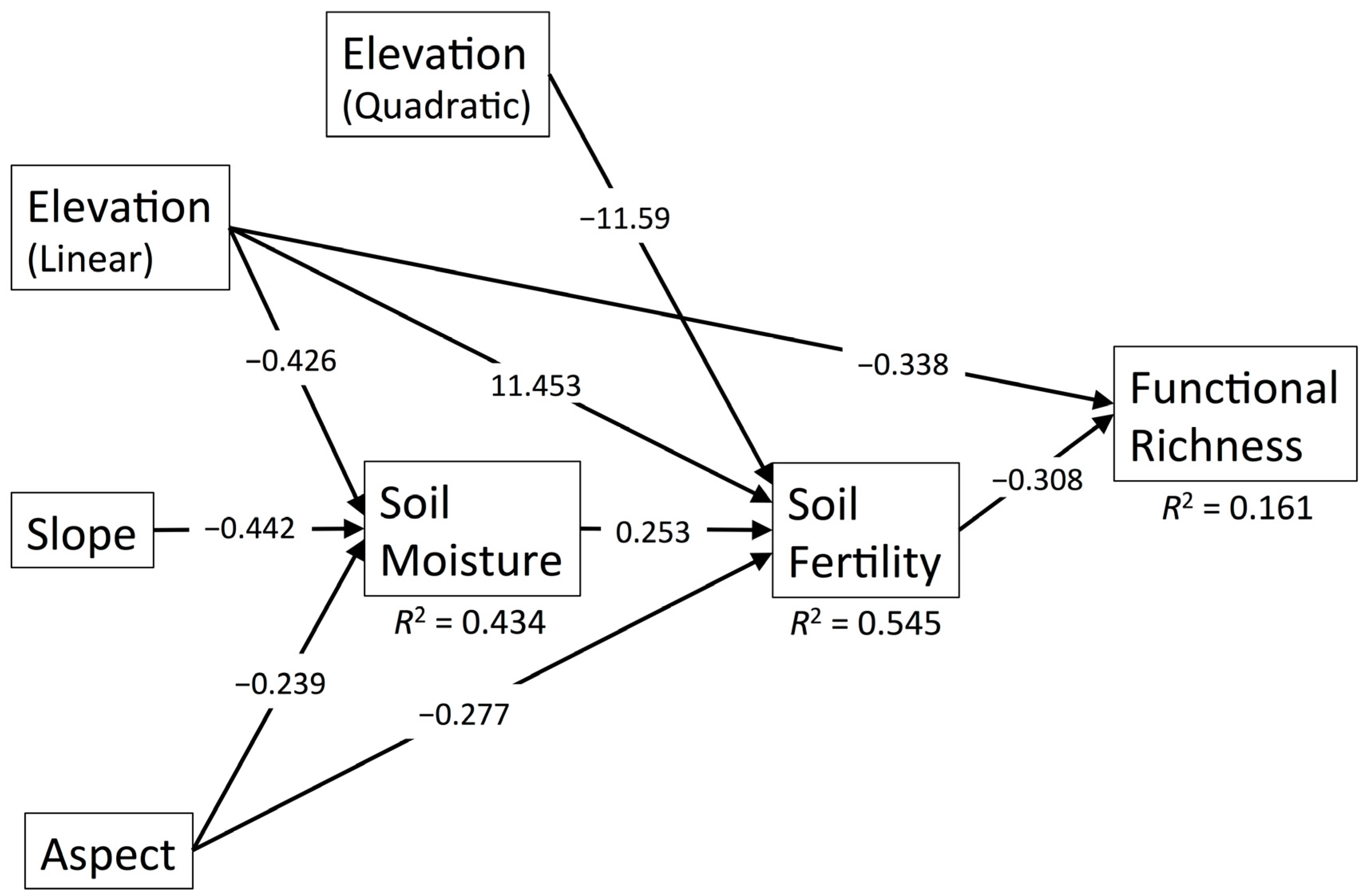
3.1. Functional Richness

The path model for functional richness explained 16.1% of its variance, and the model was a good fit (χ2 = 11.796, p = 0.623; Table 1). Variation in FRic was best explained through a combination of a direct effect of elevation and indirect effects of topography moderated through soil moisture and soil fertility (Ca, Mg, K, pH, base cation saturation; Figure 1). Functional richness had a significant inverse relationship with elevation (−0.338, p = 0.001) where FRic tended to be higher at low elevations. Soil moisture was again a moderator of all three topographic variables in this model (slope—0.442, aspect—0.239, elevation—0.426; Table 2), but the effect of moisture itself on FRic was indirect and moderated through soil fertility (−0.078). All three of these indirect pathways through moisture and soil fertility exhibited statistical relationships with p-values between 0.05 and 0.1. There were also direct links between topography and soil fertility that resulted in significant indirect effects of elevation (p = 0.006) and aspect (p = 0.024) on FRic. Soil fertility had a unimodal relationship with elevation that indicated that the highest soil fertility occurred at mid-elevation (linear 11.453, quadratic −11.59), and a linear association with aspect revealed higher soil fertility on northeast-facing (NE) slopes (−0.277; Table 2). The direct effect of soil fertility on FRic in this model was negative, indicating that functional richness is higher where soil fertility is low (−0.308).

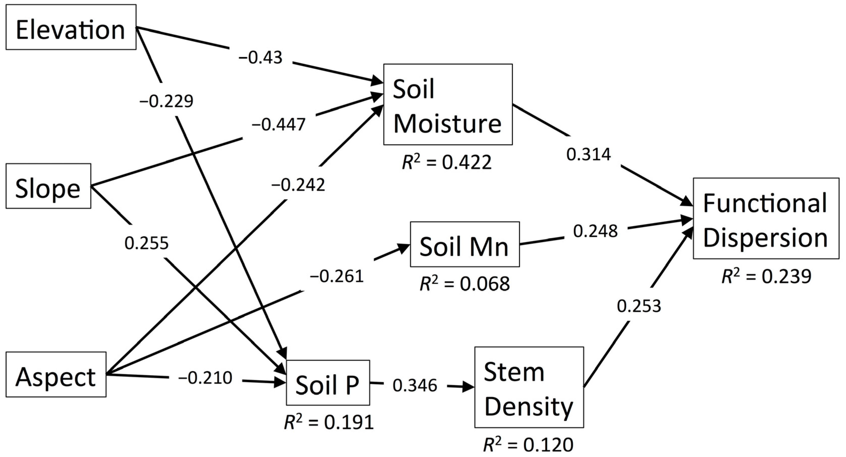
3.2. Functional Dispersion

The path model for functional dispersion was a good fit (χ2 = 12.298, p = 0.342) and explained 23.9% of the variation in FDis (Table 1). The influence of topography on FDis was moderated through indirect pathways that included soil moisture, soil P, soil Mn, and stem density (Figure 2). Soil moisture was well-explained (42.4% variance explained) by the combination of elevation (−0.43), slope (−0.447), and aspect (−0.242), and there was a significant, positive relationship between FDis and soil moisture (0.314). The indirect effects of the three topographic variables on FDis via soil moisture were all statistically significant (p < 0.05; Table 2): soil moisture appears to promote functional dispersion at low elevation, on flatter slopes, and on NE-facing aspect positions. Elevation, slope, and aspect had significant direct effects on soil P, which in turn was linked to stem density, but the indirect effects of these pathways on FDis were not statistically significant (p < 0.15; Table 2). Still, these results suggest that communities with higher FDis tend to have higher stem density, which is promoted in areas with higher available P (low elevation, steeper slopes, NE-facing). An additional indirect effect of aspect was moderated through available manganese such that NE-facing areas had higher Mn availability, which promoted FDis; this pathway was close to being statistically significant (p = 0.08; Table 2).

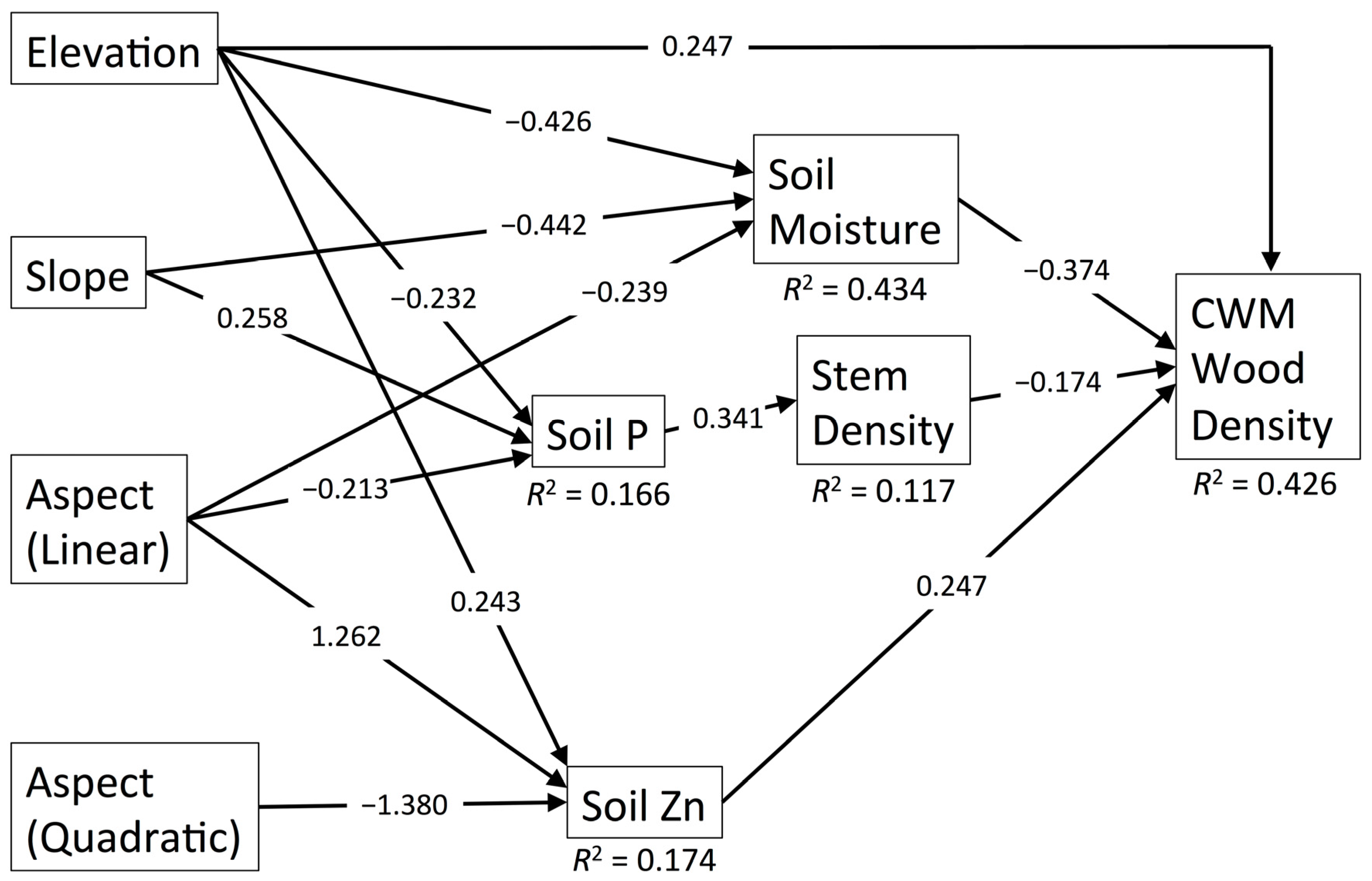
3.3. CWM Wood Density

The path model for community-weighted mean of wood density explained 42.6 % of variance but was a poor fit (χ2 = 39.075, p = 0.01; Table 1). The only direct effect of topography on CWM WD was a direct link to elevation (0.247, p = 0.011), while the indirect effects of topography were moderated through pathways involving soil moisture, soil Zn, and the effect of soil P on stem density (Figure 3). The indirect effects of elevation, slope, and aspect on WD through soil moisture were significant (p ≤ 0.02), and soil moisture had an inverse relationship with WD (−0.374; Table 3). The community-weighted mean of wood density tended to increase with decreasing soil moisture (high elevation, south-facing, steep slopes). Similar to the FDis model, there was a set of non-significant indirect pathways where stem density was positively associated with soil P, which was linked back to elevation, slope, and aspect (p < 0.19; Table 3). High WD was associated with areas of high available Zn, which tended to exist at high elevation and on east- to southeast-facing aspect positions (Table 3).

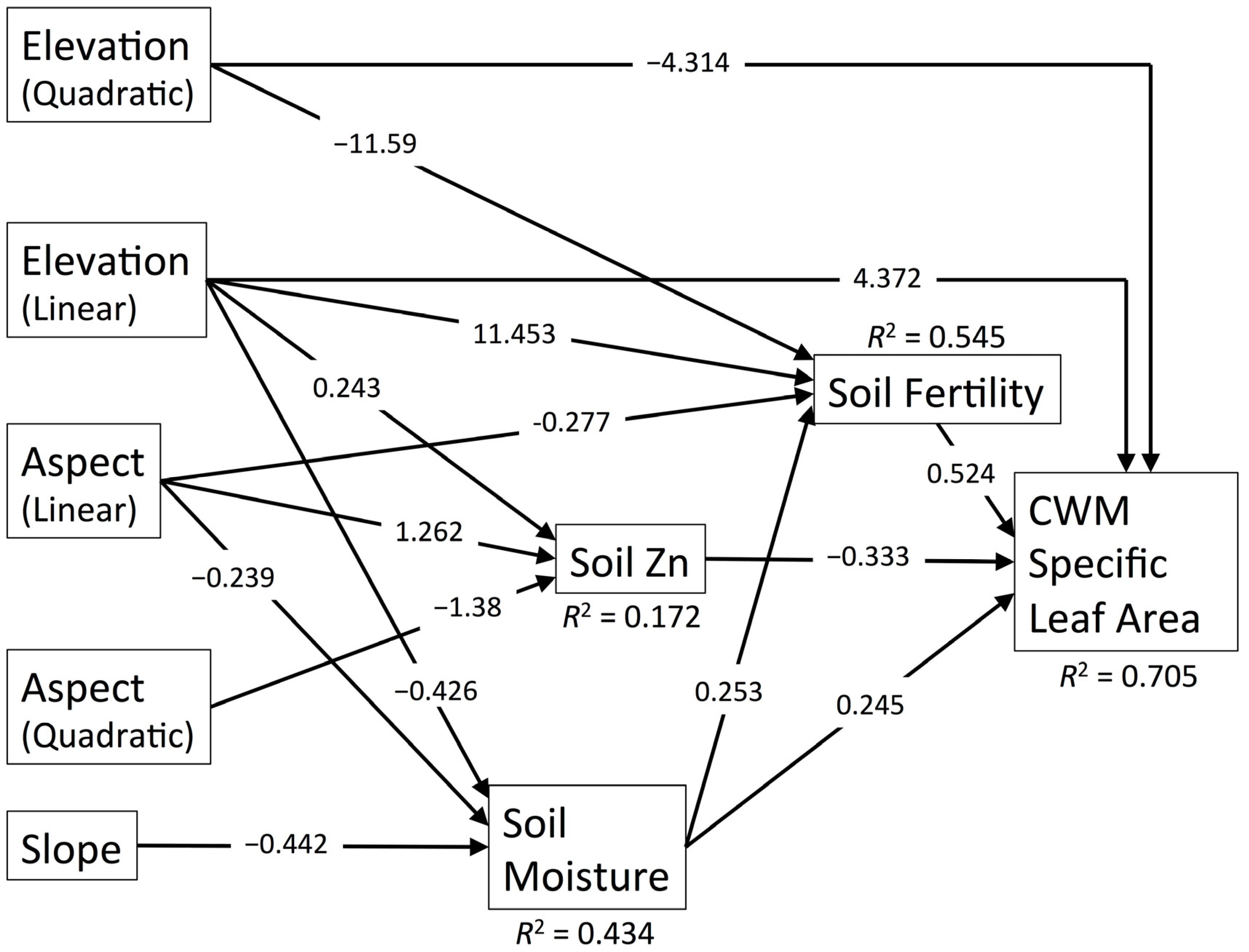
3.4. CWM Specific Leaf Area

The path model for the community-weighted mean of specific leaf area, while a poor fit (χ2 = 35.909, p = 0.011), explained 70.5% of the variance (Table 1). There was a direct effect of elevation on CWM SLA via a unimodal relationship where SLA is maximized at mid-elevation (Figure 4). SLA is positively associated with soil fertility, indicating that communities on nutrient-rich soils tend to be dominated by species with a high leaf area to dry mass ratio (broad and/or thin leaves). These areas of high soil fertility occur at mid-elevation and on NE-facing slopes, and they are also positively associated with areas of high soil moisture (low elevation, NE-facing, flatter slope angle; Table 3). SLA also exhibited a direct, positive relationship with soil moisture, indicating dominance of thicker leaf types (low leaf area to dry mass ratio) where water availability is low. Lastly, SLA was negatively associated with available soil Zn, which, in turn, was a moderator in two indirect pathways from elevation (linear relationship with soil Zn) and aspect (unimodal relationship with soil Zn similar to that described for WD; Table 3).

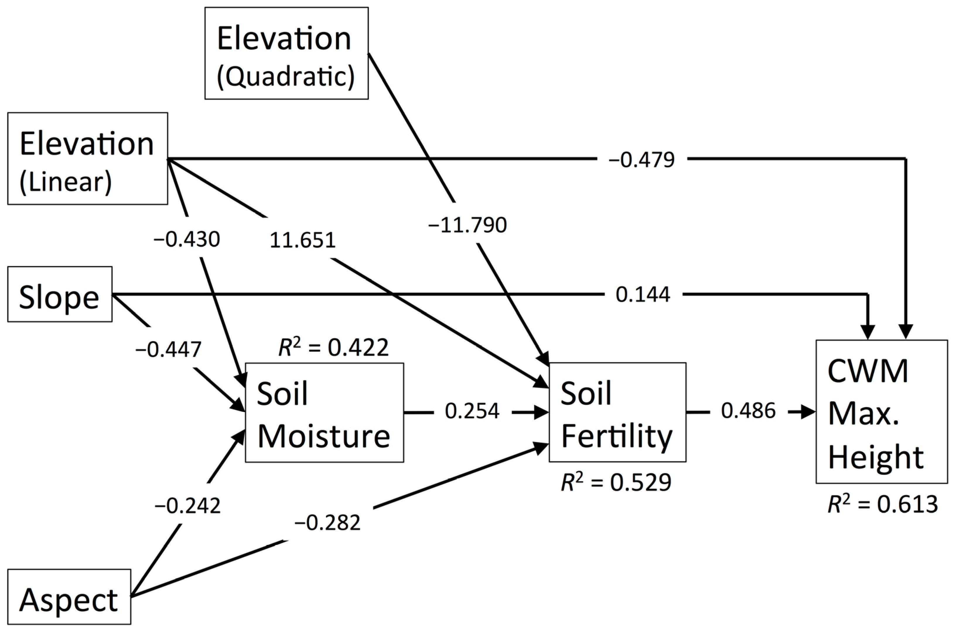
3.5. CWM Maximum Height

The path model explaining 60.3% of the variation in community-weighted mean of maximum height was a very good fit (χ2 = 10.362, p = 0.409; Table 1). Direct effects of elevation (−0.479) and slope (0.144) were present, and all indirect effects of topography were mediated through soil moisture and soil fertility (Figure 5). Maximum height was positively associated with soil fertility (0.486) such that high soil fertility promoted communities comprised of species that are taller at maturity (Table 3). As seen in previous models, soil fertility is driven by elevation (unimodal relationship), aspect (negative relationship), and soil moisture (positive relationship). Again, soil moisture is driven by all three topographic variables (Table 3).

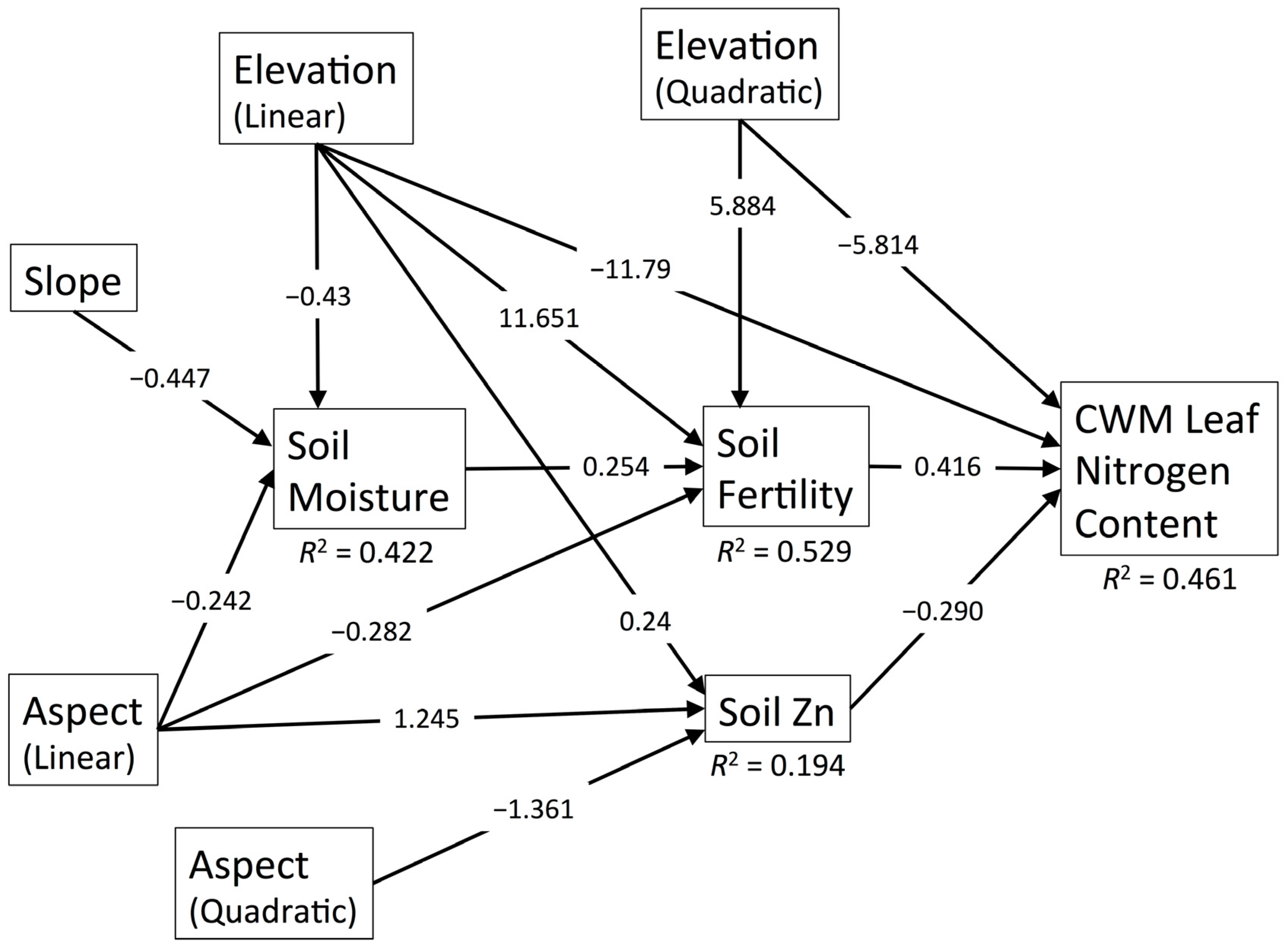
3.6. CWM Leaf Nitrogen Content
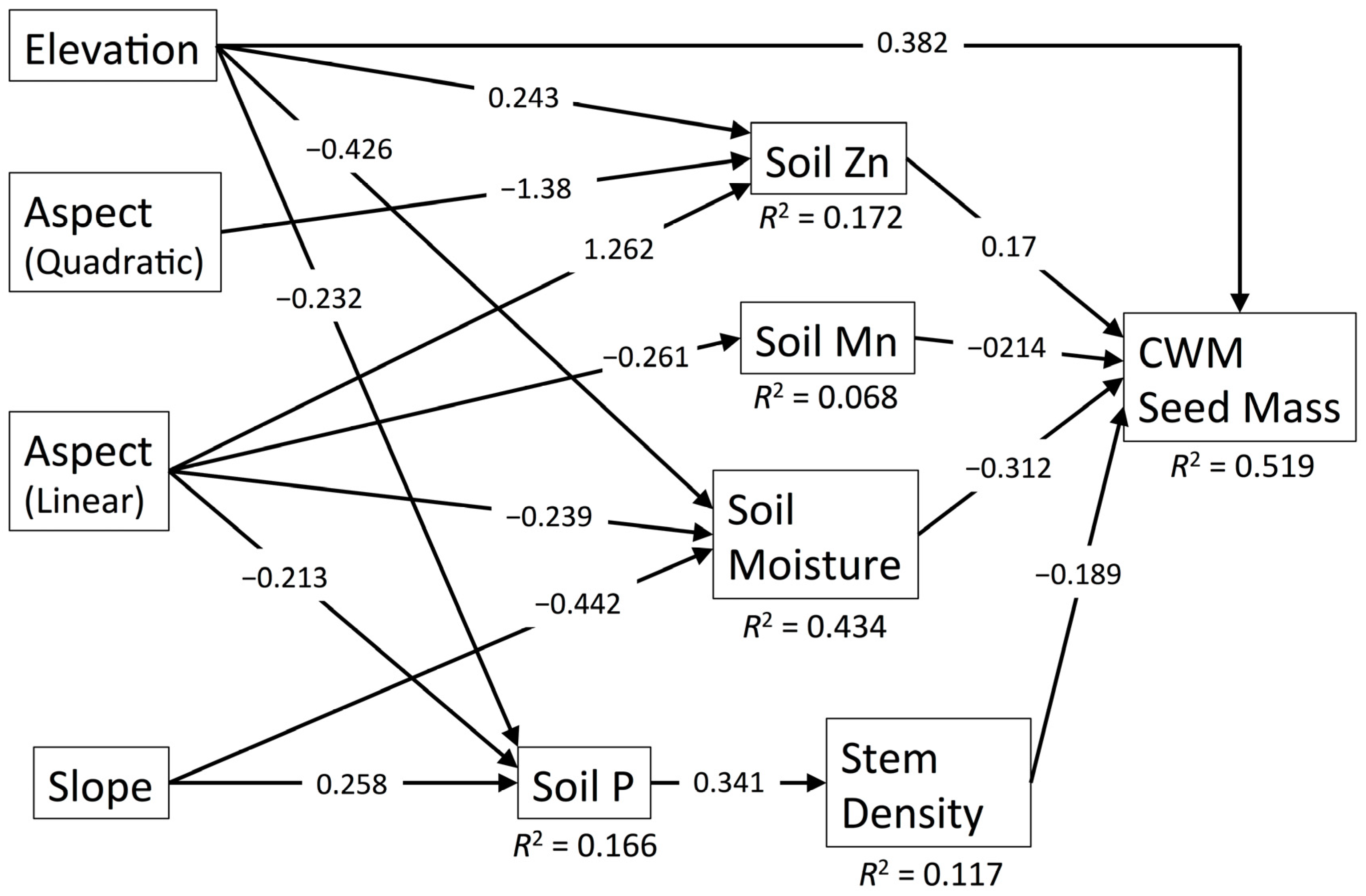
Path analysis for the community-weighted mean of leaf nitrogen content resulted in a model with poor fit (χ2 = 39.843, p = 0.005) but high total explained variance of leaf N (46.6%; Table 1). Communities with high average leaf nitrogen were found at mid-elevation, partly resulting from a direct unimodal relationship of leaf N with elevation, but also from an indirect effect of elevation mediated through soil fertility (Figure 6). High average leaf N was associated with high soil fertility occurring at mid-elevation. The indirect effect of the topography-driven soil moisture gradient was significant (p = 0.018) and mediated through soil fertility (Table 3). Leaf N was negatively associated with available Zn (−0.29), which served as a mediator of the indirect influence of elevation (linear) and aspect (unimodal). Leaf N tends to be lower in areas with high available Zn that occur at high elevation and on east- to southeast-facing slopes.

3.7. CWM Seed Mass

The path model for community-weighted mean of seed mass had somewhat of a poor fit (χ2 = 45.491, p = 0.02), but explained 51.9% of variance in seed mass (Table 1). There were several indirect pathways by which topography influenced seed mass (soil Zn, soil Mn, soil moisture, and the link between soil P and stem density), but also a positive direct effect of elevation (0.382; Figure 7). Communities with high mean seed mass were generally associated with high elevation, high available Zn, low available Mn, and low stem density. Available Zn was itself driven by a negative linear association with elevation and a unimodal association with aspect where Zn was most abundant on east- to southeast-facing slopes (Table 3). Available Mn was driven only by aspect: NE-facing slopes had higher soil Mn. Stem density was positively linked to soil P (higher available P promotes density), and soil P was driven by all three topographic variables, indicating that available P is maximized at low elevation, NE-facing aspect positions, and on steep slopes.

4. Discussion

As hypothesized (H1), the results from our old-growth Appalachian forest site were in line with the Physiological Tolerance and Stress-Dominance hypotheses; we found evidence of environmental filtering in stressful environments (drier soils with low fertility, especially on southwest-facing (SW) ridge tops) where tree communities were comprised of species with similar assemblages of morphological traits and mean trait values (CWMs) representing strategies suited for low resource availability (high wood density, low SLA, low leaf nitrogen, low maximum height, and high seed mass) [63]. High-resource environments in our site tended to support communities with greater functional dispersion, but we are unable to tease apart whether this divergence of trait syndromes is the result of competitive interactions (SDH) or the promotion of diversity with greater available resources (PTH). The positive correlation between stem density and functional dispersion may be an indication of competitive interactions driving community assembly; however, the increased FDis could also be due to a sampling effect where a greater number of individuals present increases the chances of having a broader array of functional traits present in the community. The link between stem density and soil P indicates that even if the FDis-density relationship is due to a sampling effect, there is still an underlying environmental driver.
One surprising result was that functional richness tended to be lower in areas with high soil fertility—the opposite of our hypothesized positive relationship between these two variables (H1). We believe this is the result of a strong unimodal relationship of soil fertility and elevation combined with the presence of coniferous species, Tsuga canadensis and Pinus spp., at low and high elevations (presence of Tsuga mapped by Chapman and McEwan [29]). Tsuga and Pinus have wood densities, SLAs, and leaf nitrogen contents that are lower than many, if not all, of the broad-leaved species with which they co-occur. Functional richness is not an abundance-weighted measure; therefore, the presence of even a single Tsuga or Pinus individual in any given plot increases functional richness values beyond what is found in tree communities at mid-elevation. Functional dispersion, however, is abundance-weighted, so the presence of one or even a few small individuals of Tsuga or Pinus would be outweighed by the more numerous and larger individuals of broad-leaved species. This is the case with our high elevation plots on the south-facing slope: some plots contain some small (diameter at breast height < 10 cm) individuals of Tsuga, Pinus, or both, which drive FRic values, yet these plots are dominated by large individuals of Carya spp. and Quercus spp. that drive FDis values.
The interplay among soil, topography, and microclimate is complex and results in a mosaic of local-scale habitat variation that can influence community composition, and our path models were able to capture some of these links between topography and soil variables (supporting H2). Variation in soil moisture across topographic gradients is a well-established phenomenon [5], and this association was strong in our models. Where soil moisture had a significant effect and was included in a model, over 40% of its variance was explained by the combination of slope, aspect, and elevation. We identified a positive link between soil moisture and soil fertility that is likely due to the influence of soil moisture on decomposition rates of soil organic matter and subsequent release of nutrients [64]. Interestingly, soil fertility exhibited a hump-shaped relationship with elevation. This trend may partly be driven by the presence of coniferous species at high elevation (Pinus spp.) and low elevation (Tsuga canadensis) whose leaf litter is known to lower soil pH and Ca availability [65,66], which were both included in this composite PCA axis. We expected cation exchange capacity (CEC) to be important in our models, but it was not. Cation exchange capacity is enhanced with increasing clay and organic matter contents of soils, which also contribute to greater water-holding capacity of soils. Soil pH is also linked to CEC, where greater soil acidity leads to the occupation of cation exchange sites by hydrogen ions and contributes to nutrient leaching [64,67]. Given the importance of soil moisture and soil fertility in our path models, we expected CEC to be a significant factor as well. In the initial correlation matrix used to generate our hypothesized path models, CEC was weakly correlated with stem density and aspect, but these associations were not found to be significant within the context of the path models.
The results presented in our final models should be interpreted with caution because the sample size (N = 80) was below the recommended minimum (N = 100) for SEM [59]. Chi-square goodness-of-fit tests are sensitive to sample size [59], so it is not surprising that some of our models (CWM wood density, SLA, leaf N, and seed mass) did not offer statistically significant improved fits over baseline models. Even so, the resultant p-values of the chi-square tests were not far from the p = 0.05 threshold, and other indicators were either close to or within a range of values considered “good” (comparative fit index (CFI) and standardized root mean square residual (SRMR), in particular). Achieving good fits in some of our models despite the small sample size is an indication that the relationships we have identified are robust.

5. Conclusions

The importance of abiotic gradients in structuring plant communities has long been evident to forest ecologists, and now modern analytical methods are lending statistical rigor to these assertions. Using an old-growth Appalachian forest as a model system for eastern North American forests, we used path analysis and functional diversity indices to demonstrate the role of environmental filtering in assembly of overstory tree communities. We found evidence of functional trait clustering in areas of environmental stress: low moisture and soil fertility, especially on the upper, south-facing slope of our study site. In addition, the dominant functional traits (high wood density and low SLA, in particular) in these stressful areas are indicative of a stress-tolerant life history strategy. Our models outline hypothetical causal relationships between topography and tree functional diversity, answering E. L. Braun’s call for an encompassing statistical approach, and provide a foundation for future research that tests mechanistic relationships linking topography, soil characteristics, and tree diversity in temperate forests.

Supplementary Materials

The following are available online at www.mdpi.com/1999-4907/9/1/19/s1, Table S1: Axis loadings and explained variance from principle components analysis of soil variables, Figure S1: Biplots showing plot scores (points) and soil variable scores (arrows) for the first four axes of the principle components analysis.

Acknowledgments

This is contribution No. 47 of the Lilley Cornett Woods Appalachian Ecological Research Station, Eastern Kentucky University. Much thanks goes to project initiator Robert N. Muller and all those who assisted in data collection over the years including Bridgett Abernathy, Mary Arthur, Millie Hamilton, Robert Paratley, Kaitlin Perry, Amy Reese, Rob Watts, and among many others. This work has been supported in part by the University of Dayton Office for Graduate Academic Affairs through the Graduate Student Summer Fellowship Program. The study has been supported by the TRY initiative on plant traits (http://www.try-db.org). The TRY initiative and database is hosted, developed, and maintained by J. Kattge and G. Bönisch (Max Planck Institute for Biogeochemistry, Jena, Germany). TRY is currently supported by DIVERSITAS/Future Earth and the German Centre for Integrative Biodiversity Research (iDiv) Halle-Jena-Leipzig. We thank the three anonymous reviewers who provided feedback for improving our manuscript.

Author Contributions

The authors assisted in 2010 overstory data collection (J.I.C., R.W.M.), collected soil samples (R.W.M.), and obtained the trait data (J.I.C.). J.I.C. conceived the project and performed data analyses. J.I.C. wrote the manuscript and R.W.M. proofread the manuscript.

Conflicts of Interest

The authors declare no conflict of interest.

References

  1. Braun, E.L. The vegetation of Pine Mountain, Kentucky. Am. Midl. Nat. 1935, 16, 517–565. [Google Scholar] [CrossRef]
  2. Whittaker, R.H. Vegetation of the Great Smoky Mountains. Ecol. Monogr. 1956, 26, 1–80. [Google Scholar] [CrossRef]
  3. Braun, E.L. Forests of the Cumberland Mountains. Ecol. Monogr. 1942, 12, 413–447. [Google Scholar] [CrossRef]
  4. Boerner, R.E.J. Unraveling the Gordian Knot: Interactions among vegetation, topography, and soil properties in the central and southern Appalachians. J. Torrey Bot. Soc. 2006, 133, 321–361. [Google Scholar] [CrossRef]
  5. Hutchins, R.L.; Hill, J.D.; White, E.H. The influence of soil and microclimate on vegetation of forested slopes in eastern Kentucky. Soil Sci. 1976, 121, 234–241. [Google Scholar] [CrossRef]
  6. Schmalzer, P.; Hinkle, C.; DeSelm, H. Descriminant Analysis of Cove Forests of the Cumberland Plateau of Tennessee. In Proceedings of the Central Hardwoods Forest Conference II; Pope, P., Ed.; Purdue University: West Lafayette, IN, USA, 1978; pp. 62–86. [Google Scholar]
  7. Weiher, E.; Keddy, P.A. Assembly Rules, Null Models, and Trait Dispersion, New Questions from Old Patterns. Oikos 1995, 74, 159–164. [Google Scholar] [CrossRef]
  8. Cornwell, W.K.; Schwilk, D.W.; Ackerly, D.D. A Trait-Based Test for Habitat Filtering: Convex Hull Volume. Ecology 2006, 87, 1314–1324. [Google Scholar] [CrossRef]
  9. Currie, D.J.; Mittelbach, G.G.; Cornell, H.V.; Field, R.; Guégan, J.F.; Hawkins, B.A.; Kaufman, D.M.; Kerr, J.T.; Oberdorff, T.; O’Brien, E.; et al. Predictions and tests of climate-based hypotheses of broad-scale variation in taxonomic richness. Ecol. Lett. 2004, 7, 1121–1134. [Google Scholar] [CrossRef]
  10. Coyle, J.R.; Halliday, F.W.; Lopez, B.E.; Palmquist, K.A.; Wilfahrt, P.A.; Hurlbert, A.H. Using trait and phylogenetic diversity to evaluate the generality of the stress-dominance hypothesis in eastern North American tree communities. Ecography (Cop.) 2014, 37, 814–826. [Google Scholar] [CrossRef]
  11. Sundqvist, M.K.; Sanders, N.J.; Wardle, D.A. Community and Ecosystem Responses to Elevational Gradients: Processes, Mechanisms, and Insights for Global Change. Annu. Rev. Ecol. Evol. Syst. 2013, 44, 261–280. [Google Scholar] [CrossRef]
  12. Culmsee, H.; Leuschner, C. Consistent patterns of elevational change in tree taxonomic and phylogenetic diversity across Malesian mountain forests. J. Biogeogr. 2013, 40, 1997–2010. [Google Scholar] [CrossRef]
  13. Fortunel, C.; Paine, C.E.T.; Fine, P.V.A.; Kraft, N.J.B.; Baraloto, C. Environmental factors predict community functional composition in Amazonian forests. J. Ecol. 2014, 102, 145–155. [Google Scholar] [CrossRef]
  14. Liu, J.; Yunhong, T.; Slik, J.W.F. Topography related habitat associations of tree species traits, composition and diversity in a Chinese tropical forest. For. Ecol. Manag. 2014, 330, 75–81. [Google Scholar] [CrossRef]
  15. Satdichanh, M.; Millet, J.; Heinimann, A. Using Plant Functional Traits and Phylogenies to Understand Patterns of Plant Community Assembly in a Seasonal Tropical Forest in Lao PDR. PLoS ONE 2015, 26, 1–15. [Google Scholar] [CrossRef] [PubMed] [Green Version]
  16. Shen, Y.; Yu, S.-X.; Lian, J.-Y.; Shen, H.; Cao, H.-L.; Lu, H.-P.; Ye, W.-H. Inferring community assembly processes from trait diversity across environmental gradients. J. Trop. Ecol. 2016, 32, 290–299. [Google Scholar] [CrossRef]
  17. Kraft, N.J.B.; Valencia, R.; Ackerly, D.D. Functional Traits and Niche-based Tree Community Assembly in an Amazonian Forest. Science 2008, 322, 580–582. [Google Scholar] [CrossRef] [PubMed]
  18. Lasky, J.R.; Sun, I.F.; Su, S.H.; Chen, Z.S.; Keitt, T.H. Trait-mediated effects of environmental filtering on tree community dynamics. J. Ecol. 2013, 101, 722–733. [Google Scholar] [CrossRef]
  19. Kluge, J.; Kessler, M. Phylogenetic diversity, trait diversity and niches: Species assembly of ferns along a tropical elevational gradient. J. Biogeogr. 2011, 38, 394–405. [Google Scholar] [CrossRef]
  20. Zhang, W.; Huang, D.; Wang, R.; Liu, J.; Du, N. Altitudinal patterns of species diversity and phylogenetic diversity across temperate mountain forests of northern China. PLoS ONE 2016, 11, 1–13. [Google Scholar] [CrossRef] [PubMed]
  21. Sabatini, F.M.; Burton, J.I.; Scheller, R.M.; Amatangelo, K.L.; Mladenoff, D.J. Functional diversity of ground-layer plant communities in old-growth and managed northern hardwood forests. Appl. Veg. Sci. 2014, 17, 398–407. [Google Scholar] [CrossRef]
  22. Spasojevic, M.J.; Grace, J.B.; Harrison, S.; Damschen, E.I. Functional diversity supports the physiological tolerance hypothesis for plant species richness along climatic gradients. J. Ecol. 2014, 102, 447–455. [Google Scholar] [CrossRef]
  23. Bryant, J.A.; Lamanna, C.; Morlon, H.; Kerkhoff, A.J.; Enquist, B.J.; Green, J.L. Microbes on mountainsides: Contrasting elevational patterns of bacterial and plant diversity. Proc. Natl. Acad. Sci. USA 2008, 105, 11505–11511. [Google Scholar] [CrossRef] [PubMed]
  24. Kitagawa, R.; Mimura, M.; Mori, A.S.; Sakai, A. Topographic patterns in the phylogenetic structure of temperate forests on steep mountainous terrain. AoB Plants 2015, 7, plv134. [Google Scholar] [CrossRef] [PubMed]
  25. Gilbert, G.E.; Wolfe, J.N. Soil Moisture Investigations at Neotoma, a Forest Bioclimatic Laboratory in Central Ohio. Ohio J. Sci. 1959, 59, 38–46. [Google Scholar]
  26. Franzmeier, D.; Pederson, E.; Longwell, T.; Byrne, J.; Losche, C. Properties of Some Soils in the Cumberland Plateau as Related to Slope Aspect and Position. Soil Sci. Soc. Am. Proc. 1969, 33, 755–761. [Google Scholar] [CrossRef]
  27. Losche, C.; McCracken, R.; Davey, C. Soils of Steeply Sloping Landscapes in Southern Appalachian Mountains. Soil Sci. Soc. Am. Proc. 1970, 4, 473–478. [Google Scholar] [CrossRef]
  28. Hairston, A.; Grigal, D. Topographic influences on soils and trees within single mapping units on a sandy outwash landscape. For. Ecol. Manag. 1991, 43, 35–45. [Google Scholar] [CrossRef]
  29. Chapman, J.I.; McEwan, R.W. Thirty Years of Compositional Change in an Old-Growth Temperate Forest: The Role of Topographic Gradients in Oak-Maple Dynamics. PLoS ONE 2016, 11, e0160238. [Google Scholar] [CrossRef] [PubMed]
  30. McEwan, R.W.; Muller, R.N. Spatial and temporal dynamics in canopy dominance of an old-growth central Appalachian forest. Can. J. For. Res. 2006, 36, 1536–1550. [Google Scholar] [CrossRef]
  31. McEwan, R.W.; Muller, R.N.; McCarthy, B.C. Vegetation-Environment Relationships Among Woody Species in Four Canopy-Layers in an Old-Growth Mixed Mesophytic Forest. Castanea 2005, 70, 32–46. [Google Scholar] [CrossRef]
  32. Chapman, J.I.; McEwan, R.W. Spatiotemporal dynamics of a and β diversity across topographic gradients in the herbaceous layer of an old-growth deciduous forest. Oikos 2013, 122, 1679–1686. [Google Scholar] [CrossRef]
  33. Martin, W.H. The Lilley Cornett Woods: A Stable Mixed Mesophytic Forest in Kentucky. Bot. Gaz. 1975, 136, 171–183. [Google Scholar] [CrossRef]
  34. Trewartha, G. An Introduction to Climate, 4th ed.; McGraw and Hill: New York, NY, USA, 1968. [Google Scholar]
  35. Hill, J.D. Climate of Kentucky, Report No 221; University of Kentucky College of Agriculture: Lexington, KY, USA, 1976. [Google Scholar]
  36. Muller, R.N. Vegetation Patterns in the Mixed Mesophytic Forest of Eastern Kentucky. Ecology 1982, 63, 1901–1917. [Google Scholar] [CrossRef]
  37. Braun, E.L. Deciduous Forests of Eastern North America; The Blakiston Company: Philadelphia, PA, USA, 1950. [Google Scholar]
  38. Carter, M. Soil Sampling and Methods of Analysis; Lews Publishing: Boca Raton, FL, USA, 1993. [Google Scholar]
  39. McEwan, R.W.; Chapman, J.I.; Muller, R.N. 2010 Lilley Cornett Woods Overstory Data. Data Files: Big Everidge Hollow Permanent Plots. Available online: http://ecommons.udayton.edu/mcewanlab_1_data/1 (accessed on 5 January 2018). [CrossRef]
  40. McEwan, R.W.; Chapman, J.I.; Muller, R.N. 2001 Lilley Cornett Woods Soil Data. Data Files: Big Everidge Hollow Permanent Plots. Available online: http://ecommons.udayton.edu/mcewanlab_1_data/6 (accessed on 5 January 2018). [CrossRef]
  41. McEwan, R.W.; Chapman, J.I.; Muller, R.N. Lilley Cornett Woods Plot Information and Topography Data. Data Files: Big Everidge Hollow Permanent Plots. Available online: http://ecommons.udayton.edu/mcewanlab_1_data/8 (accessed on 5 January 2018). [CrossRef]
  42. Wright, I.J.; Reich, P.B.; Westoby, M.; Ackerly, D.D.; Baruch, Z.; Bongers, F.; Cavender-Bares, J.; Chapin, T.; Cornelissen, J.H.C.; Diemer, M.; et al. The worldwide leaf economics spectrum. Nature 2004, 428, 821–827. [Google Scholar] [CrossRef] [PubMed]
  43. Kattge, J.; Diaz, S.; Lavorel, S.; Prentice, I.C.; Leadley, P.; Bonisch, G.; Garnier, E.; Westoby, M.; Reich, P.B.; Wright, I.J.; et al. A global database of plant traits. Glob. Chang. Biol. 2011, 17, 2905–2935. [Google Scholar] [CrossRef] [Green Version]
  44. Kattge, J.; Knorr, W.; Raddatz, T.; Wirth, C. Quantifying photosynthetic capacity and its relationship to leaf nitrogen content for global-scale terrestrial biosphere models. Glob. Chang. Biol. 2009, 15, 976–991. [Google Scholar] [CrossRef]
  45. Bolster, K.; Martin, M.; Aber, J. Determination of carbon fraction and nitrogen concentration in tree foliage by near infrared reflectance: Comparison of statistical methods. Can. J. For. Res. 1996, 26, 590–600. [Google Scholar] [CrossRef]
  46. Chave, J.; Coomes, D.; Jansen, S.; Lewis, S.L.; Swenson, N.G.; Zanne, A.E. Towards a worldwide wood economics spectrum. Ecol. Lett. 2009, 12, 351–366. [Google Scholar] [CrossRef] [PubMed]
  47. Harmon, M.E.; Woodall, C.W.; Fasth, B.; Sexton, J. Woody Detritus Density and Density Reduction Factors for Tree Species in the United States: A Synthesis; USDA Forest Service Northern Research Station: Newtown Square, PA, USA, 2008; p. 84.
  48. Zanne, A.E.; Lopez-Gonzalez, G.; Coomes, D.A.; Ilic, J.; Jansen, S.; Lewis, S.L.; Miller, R.B.; Swenson, N.G.; Wiemann, M.C.; Chave, J. Data from: Towards a worldwide wood economics spectrum. Dryad Digit. Repos. 2009. [Google Scholar] [CrossRef]
  49. Moles, A.T.; Westoby, M. Seed size and plant strategy across the whole life cycle. Oikos 2006, 113, 91–105. [Google Scholar] [CrossRef]
  50. Kew, R.B.G. Seed Information Database (SID). Version 7.1. Available online: http://data.kew.org/sid/ (accessed on 17 July 2014).
  51. Moles, A.T.; Warton, D.I.; Warman, L.; Swenson, N.G.; Laffan, S.W.; Zanne, A.E.; Pitman, A.; Hemmings, F.A.; Leishman, M.R. Global patterns in plant height. J. Ecol. 2009, 97, 923–932. [Google Scholar] [CrossRef]
  52. USDA, NRCS. The PLANTS Database; National Plant Data Team: Greensboro, NC, USA. Available online: http://plants.usda.gov (accessed on 6 August 2014).
  53. Laliberté, E.; Legendre, P. A distance-based framework for measuring functional diversity from multiple traits. Ecology 2010, 91, 299–305. [Google Scholar] [CrossRef] [PubMed]
  54. Laliberté, E.; Legendre, P.; Shipley, B. FD: Measuring Functional Diversity from multiple traits, and other tools for functional ecology. R package version 1.0–1.2. 2014. Available online: https://cran.r-project.org/web/packages/FD/FD.pdf (accessed on 14 October 2014).
  55. Mason, N.W.H.; Mouillot, D.; Lee, W.G.; Wilson, J.B. Functional richness, functional evenness and functional divergence: The primary components of functional diversity. Oikos 2005, 111, 112–118. [Google Scholar] [CrossRef]
  56. Garnier, E.; Cortez, J.; Billès, G.; Navas, M.L.; Roumet, C.; Debussche, M.; Laurent, G.; Blanchard, A.; Aubry, D.; Bellmann, A.; et al. Plant functional markers capture ecosystem properties during secondary succession. Ecology 2004, 85, 2630–2637. [Google Scholar] [CrossRef]
  57. Mason, N.W.H.; De Bello, F.; Mouillot, D.; Pavoine, S.; Dray, S. A guide for using functional diversity indices to reveal changes in assembly processes along ecological gradients. J. Veg. Sci. 2013, 24, 794–806. [Google Scholar] [CrossRef]
  58. Swenson, N.G. Functional and Phylogenetic Ecology in R; Springer-Verlag: New York, NY, USA, 2014. [Google Scholar]
  59. Kline, R.B. Principles and Practice of Structural Equation Modeling, 2nd ed.; The Guilford Press: New York, NY, USA, 2005. [Google Scholar]
  60. Denslow, J.S. Disturbance and Diversity in Tropical Rain Forests: The Density Effect. Ecol. Appl. 1995, 5, 962–968. [Google Scholar] [CrossRef]
  61. Hu, L.T.; Bentler, P.M. Cutoff criteria for fit indexes in covariance structure analysis: Conventional criteria versus new alternatives. Struct. Equ. Model. 1999, 6, 1–55. [Google Scholar] [CrossRef]
  62. Rosseel, Y. lavaan: An R Package for Structural Equation Modeling. J. Stat. Softw. 2012, 48, 1–36. [Google Scholar] [CrossRef]
  63. Stahl, U.; Kattge, J.; Reu, B.; Voigt, W.; Ogle, K.; Dickie, J.; Wirth, C. Whole-plant trait spectra of North American woody plant species reflect fundamental ecological strategies. Ecosphere 2013, 4, 128. [Google Scholar] [CrossRef]
  64. Barbour, M.G.; Burk, J.H.; Pitts, W.D.; Gilliam, F.S.; Schwartz, M.W. Terrestrial Plant Ecology, 3rd ed.; Bejamin Cummings: Menlo Park, CA, USA, 1999. [Google Scholar]
  65. Finzi, A.C.; Canham, C.D.; van Breemen, N. Canopy Tree-Soil Interactions within Temperate Forests: Species Effects on pH and Cations. Ecol. Appl. 1998, 8, 447–454. [Google Scholar]
  66. Alban, D.H. Effects of Nutrient Accumulation by Aspen, Spruce, and Pine on Soil Properties. Soil Sci. Soc. Am. J. 1982, 46, 853–861. [Google Scholar] [CrossRef]
  67. McFee, W.W.; Kelly, J.M.; Beck, R.H. Acid precipitation effects on soil pH and base saturation of exchange sites. Water Air Soil Pollut. 1977, 7, 401–408. [Google Scholar] [CrossRef]
Figure 1. Path diagram for functional richness (FRic). Standardized path coefficients are given. R2 values are total explained variance.
Forests 09 00019 g001
Figure 2. Path diagram for functional dispersion (FDis). Standardized path coefficients are given. R2 values are total explained variance.
Forests 09 00019 g002
Figure 3. Path diagram for community-weighted mean wood density. Standardized path coefficients are given. R2 values are total explained variance.
Forests 09 00019 g003
Figure 4. Path diagram for community-weighted mean specific leaf area. Standardized path coefficients are given. R2 values are total explained variance.
Forests 09 00019 g004
Figure 5. Path diagram for community-weighted mean maximum height. Standardized path coefficients are given. R2 values are total explained variance.
Forests 09 00019 g005
Figure 6. Path diagram for community-weighted mean leaf nitrogen content. Standardized path coefficients are given. R2 values are total explained variance.
Forests 09 00019 g006
Figure 7. Path diagram for community-weighted mean seed mass. Standardized path coefficients are given. R2 values are total explained variance.
Forests 09 00019 g007
Table 1. Path Analysis model results. Root mean square error of approximation (RMSEA) < 0.05, standardized root mean square residual (SRMR) < 0.08, and comparative fit index (CFI) > 0.95 indicate good fit.
Diversity Metricχ2dfpRMSEASRMRCFIR2
FRic12.298110.3420.0380.0740.9980.161
FDis11.796140.6230.0000.0541.0000.239
CWM WD39.075210.0100.1040.0870.9500.426
CWM SLA35.909190.0110.1050.0860.9820.705
CWM Leaf N39.843200.0050.1110.0780.9780.466
CWM Max. Ht.10.362100.4090.0210.0730.9990.603
CWM Seed Mass45.491280.0200.0880.0770.9540.519
p-values greater than 0.05 indicate a significantly better fit than baseline models. CWM: community-weighted mean; WD: wood density; SLA: specific leaf area; Leaf N: leaf nitrogen content; Max. Ht.: maximum height.
Table 2. Direct, indirect, and total path coefficients (standardized) of path models containing overall functional diversity measures: functional richness (FRic) and functional dispersion (FDis). Soil fertility is a principle components analysis (PCA) axis representing soil pH, Base Cation Saturation, and available Ca, Mg, and K.
PredictorPathwayFRicFDis
CoeffpCoeffp
Elevation (Linear)Direct−0.3380.001--
Indirect through Soil Moisture--−0.1350.007
Indirect through Soil Moisture and Soil Fertility0.0330.055--
Indirect through Soil Fertility−3.530.006--
Indirect through Soil P and Stem Density--−0.0200.130
Total−3.8350.003−0.1550.003
Elevation (Quadratic)Indirect through Soil Fertility3.5720.006--
Aspect (Linear)Indirect through Soil Moisture−0.0760.035
Indirect through Soil Moisture and Soil Fertility0.0190.094--
Indirect through Soil P and Stem Density--−0.0180.148
Indirect through Soil Fertility0.0850.024--
Indirect through Soil Mn--−0.0650.080
Total0.1040.015−0.1590.002
SlopeIndirect through Soil Moisture--−0.1400.006
Indirect through Soil Moisture and Soil Fertility0.0340.054--
Indirect through Soil P and Stem Density--0.0220.114
Total0.0340.054−0.1180.027
Stem DensityDirect--0.2530.010
Soil MoistureDirect--0.3140.001
Indirect through Soil Fertility−0.0780.039--
Soil FertilityDirect−0.3080.003--
Indirect through Stem Density--0.0880.042
Soil MnDirect--0.2480.011
Table 3. Direct, indirect, and total path coefficients (standardized) of path models for community-weighted mean trait values (CWM). Traits were wood density (WD), specific leaf area (SLA), maximum height (Max. Ht.), leaf nitrogen content (Leaf N), and seed mass. Soil Fertility is a PCA axis representing soil pH, Base Cation Saturation, and available Ca, Mg, and K.
PredictorPathwayWDSLAMax. Ht.Leaf NSeed Mass
CoeffpCoeffpCoeffpCoeffpCoeffp
Elevation (Linear)Direct0.2470.0114.3720.005−0.4850.0005.8560.0040.3820.000
Indirect through Soil Moisture0.1590.002−0.1040.005----0.1330.003
Indirect through Soil Moisture and Soil Fertility--−0.0560.019−0.0540.018−0.0450.032--
Indirect through Soil Fertility--6.0030.0005.7380.0004.8190.000--
Indirect through Soil Zn0.0600.068−0.0810.029--−0.0690.0510.0410.112
Indirect through Soil P and Stem Density0.0140.1680.0150.139
Total0.4800.00010.130.0005.1990.00010.560.0000.5720.000
Elevation (Quadratic)Direct--−4.3140006--−5.7870.005--
Indirect through Soil Fertility--−6.0750.000−5.8070.000−4.8770.000--
Total--−10.390.000−5.8070.000−10.660.000--
Aspect (Linear)Indirect through Soil Moisture0.0900.020−0.0590.030----0.0750.025
Indirect through Soil Moisture and Soil Fertility--−0.0320.053−0.0300.051−0.0250.069--
Indirect through Soil P and Stem Density0.0130.182------0.0140.154
Indirect through Soil Fertility--−0.1450.002−0.1390.002−0.1170.008--
Indirect through Soil Zn0.3120.042−0.4200.010--−0.3590.0270.2150.085
Indirect through Soil Mn--------0.0560.069
Total0.4140.009−0.6560.000−0.1690.000−0.5010.0030.3590.007
Aspect (Quadratic)Indirect through Soil Zn−0.3410.0340.4600.006--0.3930.020−0.2350.076
SlopeDirect----0.1460.040----
Indirect through Soil Moisture0.1650.001−0.1080.005----0.1380.003
Indirect through Soil Moisture and Soil Fertility--−0.0590.018−0.0560.017−0.0470.031--
Indirect through Soil P and Stem Density−0.0150.153------−0.0170.123
Total0.1500.005−0.1670.0010.0900.223−0.0470.0310.1210.010
Stem DensityDirect−0.1740.041------−0.1890.015
Soil MoistureDirect−0.3740.0000.2450.001----−0.3120.000
Indirect through Soil Fertility--0.1320.0080.1270.0070.1060.018--
Total−0.3740.0000.3770.0000.1270.0070.1060.018--
Soil FertilityDirect--0.5240.0000.5010.0000.4210.000--
Soil ZnDirect0.2470.005−0.3330.000--−0.2850.0010.1700.033
Soil PIndirect through Stem Density−0.0590.083------−0.0650.052
Soil MnDirect--------−0.2140.006

