
Dual-Filter Estimation for Rotating-Panel Sample Designs

Southern Research Station, USDA Forest Service, 200 WT Weaver Blvd., Asheville, NC 28804, USA
Forests 2017, 8(6), 192; https://doi.org/10.3390/f8060192
Submission received: 11 April 2017
/
Revised: 26 May 2017
/
Accepted: 31 May 2017
/
Published: 2 June 2017
Abstract
:Dual-filter estimators are described and tested for use in the annual estimation for national forest inventories. The dual-filter approach involves the use of a moving widow estimator in the first pass, which is used as input to Theil’s mixed estimator in the second pass. The moving window and dual-filter estimators are tested along with two other estimators in a sampling simulation of 152 simulated populations, which were developed from data collected in 38 states and Puerto Rico by the Forest Inventory and Analysis Program of the USDA Forest Service. The dual-filter estimators are shown to almost always provide some reduction in mean squared error (MSE) relative to the first pass moving window estimators.
1. Introduction
A rotating panel design for re-measured ground observations has replaced what are known as periodic inventory designs in the United States and elsewhere in an effort to improve the annual estimation of forest attributes. Rotating panel designs pose unique advantages and challenges with respect to making annual estimates of population phenomena. This work focuses on one of the most basic of those challenges, faced by virtually all organizations conducting national forest inventory (NFI) efforts. That challenge stems from the common practice in NFIs to subdivide the land area into estimation units. These units usually have some historical significance and often some biological and ecological significance as well, at least at a coarse scale. In many cases, as in the US, they were formed decades ago and were large enough to include enough sample elements in a periodic inventory to produce estimates of most attributes at a desired level of confidence. In a periodic inventory, the sampling effort for an estimation unit is concentrated in a single year. In the rotating panel sample design, the sampling effort for the full inventory is spread over P years, with a unique sample panel observed in each of those years, in succession, creating a small sample realization in any particular year. Nevertheless, the incorporation of annual inventories has created an expectation of high-quality annual estimates within historical estimation units. In the US, in anticipation of this expectation, both prior to and in the early years of incorporation of the rotating panel design, there was a concentration of effort on the question of how to best combine the data from successive years to form annual estimates. In the examination of potential estimators, I ask the reader to keep in mind that estimators used in the NFI usually run within bulk data processing programs that often are not, and possibly cannot, be monitored, due to the large amount of data that is being processed at one time. This suggests the need for a default estimator; that is, one that is resorted to, within the program, if all else fails. Such a default had been suggested for use by the USDA Forest Service’s Forest Inventory and Analysis (FIA) Program and presented in Bechtold and Patterson [1]. That estimator is a moving average estimator, applied in a non-standard way, specifically to the end of the period, rather than the usual middle of the period (or window), and can be expressed as:
where P is the number of panels (and years, given that one panel per year is measured), t is the year of interest, and yi is the observation of the variable of interest in year i. This end of period estimator (FIA_EoP) is by now well-known: it will usually have very low variance because it uses all of the available data, but will be biased in the presence of a non-zero trend. When it was chosen as the default estimator, it was hoped that the bias would usually be small enough to be unimportant relative to the significant reduction in variance. Below we will employ a natural statistic, the mean squared error (), for investigating how well this hope has been realized. The advantage that we have today, which we did not have when Equation (1) was chosen as the default estimator, is that in some areas in the US, we have data that has been collected under the rotating-panel design for almost two decades that we can use to more thoroughly test proposed estimation systems. In this paper, I test the performance of FIA_EoP and other estimators of annual volume in a sampling simulation of 152 populations, each built from the data observed on a unique FIA estimation unit. Two other classes of estimators are considered here. The first class of estimators includes specific applications of the well-known moving window estimator:
where k is the window width in years, which in this paper is an odd integer. In the applications below, k = 3, 5, and 9. Note that the vector of estimates from each application () will be shorter than the number of input years by (k − 1). Therefore, there are no estimates for the first 0.5(k − 1) and the last 0.5(k − 1) years. If the number of input years is T, MW3 will provide estimates for the years 2 through T − 1, MW5 will produce estimates for the years 3 through T − 2, and MW9 will provide estimates for the years 5 through T − 4.
The second set of estimators can best be described as dual-filter estimators, in which two simple filters are applied in succession to easily achieve a higher-order model. I test three such dual filter estimators here. In each I use one of the three applications of the moving window estimator above for the first filter. For the second filter, I use the results of each moving window estimator in a variant of Theil’s mixed estimator (Theil [2]). The specific variant uses the quadratic model described in Van Deusen [3,4], who was the first to propose mixed estimators for continuous forest inventory designs. Although not given a name, the dual-filter approach was first recommended for this forest monitoring design in Roesch [5], as a way of reducing the variance of small-area inputs into the mixed estimator.
For each dual-filter estimator, with a first filter of , let
- n = T − k + 1;
- = an n row by n column co-variance matrix for ;
- = an (n − 3) row by (n − 3) column sub-matrix of , using rows and columns from 4 to n;
- R = an (n − 3) row by n column constraint matrix, appropriate for the quadratic model, which has zeros everywhere except that each row t has the sequence [1,−3,3,−1] beginning in column t.
The dual filter estimator is then:
Here, as in Van Deusen [4], sample statistics provide everything for the estimator in Equation (3) except for the value of the unknown parameter p, which is estimated with maximum likelihood, the details of which can be found in that reference.
The most serious limitation for both the MWx and the MixMWx estimators is that they do not provide estimates for the first 0.5(k − 1) and the last 0.5(k − 1) years in the series. The six estimators (MW3, MW5, MW9, MixMW3, MixMW5, and MixMW9) were supplemented through recursion to provide estimates for the otherwise missing years, under the assumption that the trend estimated in the initial and final estimated years remained constant through the estimator’s initial and ending “missing” years, respectively. To supplement estimator E to provide estimates for the first 0.5(k − 1) and the last 0.5(k − 1) years of T years, apply the algorithm as follows.
Let:
dl = E[0.5(k − 1) + 2] − E[0.5(k − 1) + 1]
and then for t = 0.5(k − 1) to 1,
E[t] = E[t + 1] − dl.
Next, let:
du = E[T − 0.05(k − 1)] − E[T − (0.5(k − 1) + 1)];
and then for (t = T − (0.5(k − 1) − 1) to T),
E[t] = E[t − 1] + du.
The missing early years for FIA_EoP were not supplemented for two reasons. First and foremost, it would be counter to the philosophy and intent of that estimator because the estimator is only intended to provide an estimate for the most recent year of data collection. Second it would be an extremely long series to supplement under the assumption used to supplement the other estimators.
These seven estimators and their advantages relative to the annual sample mean and to each other are compared in the simulation described below.
2. Materials and Methods
2.1. Simulated Populations
The data from each of the 152 FIA estimation units were used to construct a simulated population. Each of these populations is intended to reflect the population characteristics in the land area of the estimation unit. All of the states and territories covered by the FIA in the period from 1995 to 2015 were considered for this study, however, some states and territories did not yet have enough data in all estimation units to construct a general set of populations for the unit. This resulted in the use of data that came from the 152 estimation units in 38 states and Puerto Rico (listed in Appendix A). The methods used to construct the populations were used previously in Roesch [5,6], and Roesch et al. [7]. The earlier studies used seed data from much smaller geographic areas. Because the seed data itself for this study was so much more diverse, I did not construct multiple populations from a single dataset, as in earlier studies, but rather treated each estimation unit as a unique population. Each population was constructed to represent the set of forested conditions within each estimation unit. Using the methods described in Roesch [8], the data from each plot in an estimation unit were used to create a sequence of 21 successive, annual values from each ground plot, for each variable of interest. That is, each plot was converted into a 21-year, 1-hectare population of values of interest, which is label as Set 1. The reader interested in more detail of the exact method is referred to the prior publication. It is assumed that each line in Set 1 represents a condition class and that a condition class is composed of similar but unique elements or land segments that have had a similar but unique developmental series through the 21-year period. To achieve this diverse set of elements, random variance was applied at two levels to Set 1. This was done 100 times, resulting in the population for each estimation unit. In level 1, in order to add variance but maintain trend, all values for each growth component on each hectare were multiplied by a unique random variate, drawn from an N (1, 0.025) distribution. A second level of variance was effected temporally by multiplying the result of level 1 for each annual value on each hectare by a unique random variate drawn from an N (1, 0.0025) distribution. The initial volume matrix was then re-calculated, starting at the first year of non-zero volume observation for each line and applying the growth components recursively. Note that the population diversity being created here through the use of these random variates is a simplification of reality in that this diversity is assumed to have existed at different levels in each of the original sampled populations, but was not observed. Although not conducted for this study, different levels of spatial diversity could be simulated by adjusting the standard deviation of the normal variate in level 1, while different levels of trend or temporal diversity could be simulated by adjusting the standard deviation of the normal variate in level 2. The practitioner who would endeavor to do this in a particular population should be aware that setting the standard deviation too high at level 2 would tend to obfuscate the temporal trend and possibly result in unrealistic annual changes in volume in smaller populations.
2.2. Sampling the Simulated Populations
I used the method described in Roesch et al. [7] to simulate sampling errors. Each sampling simulation consisted of 1000 iterations of a 10% sample each (without replacement) from the population. Additional sampling error was introduced by multiplying a unique random normal deviate of mean 1 and standard deviation of 0.01, by each observation of volume. The class of forest monitoring designs being simulated and discussed here provide direct annual estimates of standing volume. For each iterate and for each year, the mean, bias, and mean squared error (MSE) were calculated for each estimator over each population. The bias is calculated as:
where is the sample estimate of the variable, X, in population P for estimator E for a particular year for iterate i. The mean squared error is:
The overall weighted mean, bias and MSE were used as criteria for judging the effectiveness of the estimators. Although examining both the mean and the bias is somewhat redundant, plotting the estimator means relative to the true population means can sometimes be more informative than plotting the bias, especially when the estimators are affected by population trends. The mean, bias, and MSE of each population are weighted in the final statistics to account for the differences in population sizes. Each population mean () and bias (BP) is weighted by the proportion of the population area () to the total area of all populations (A), and each population (MSEP) is weighted by the proportion of its area squared to the sum of the squares of population areas. To be clear, the overall weighted mean is:
The overall weighted bias is:
and the overall weighted MSE is:
3. Results
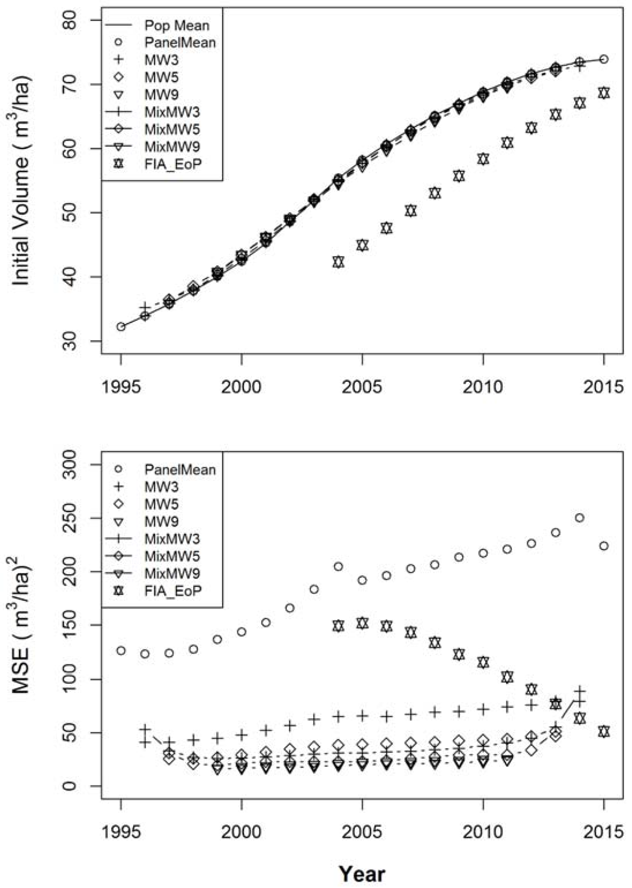
The results of the simulations are presented in Figure 1 and Figure 2. Figure 1 gives the weighted means of the volume estimators relative to the overall population mean in the top graph and the overall weighted mean squared errors in the bottom graph. The results for the estimators are plotted over the natural (not-supplemented) range of each estimator, as defined. As expected, all of the estimators except for FIA_EoP show very little bias in the annual estimates. The FIA_EoP estimator also shows bias being reduced as time progresses. This can only be a result of a reduction of the slope of the overall population trend. As the rate of change in the population reduces, the bias in FIA_EoP will likewise be reduced. The bottom graph shows that the MSEs are lower for all of the estimators relative to the MSE of the annual population mean. Except for the first and last year in the range of each estimator MixMW3 and MixMW5 have lower MSEs than their corresponding input estimators, MW3 and MW5. MixMW3 is also almost always lower in MSE than MW5, suggesting that the dual estimation approach shows an advantage that somewhat overrides the amount of input data. There are only very small differences in the results for MW9 and MixMW9, with most of the MSEs being just slightly lower for MixMW9. Both MW9 and MixMW9 have lower MSEs than the other estimators.
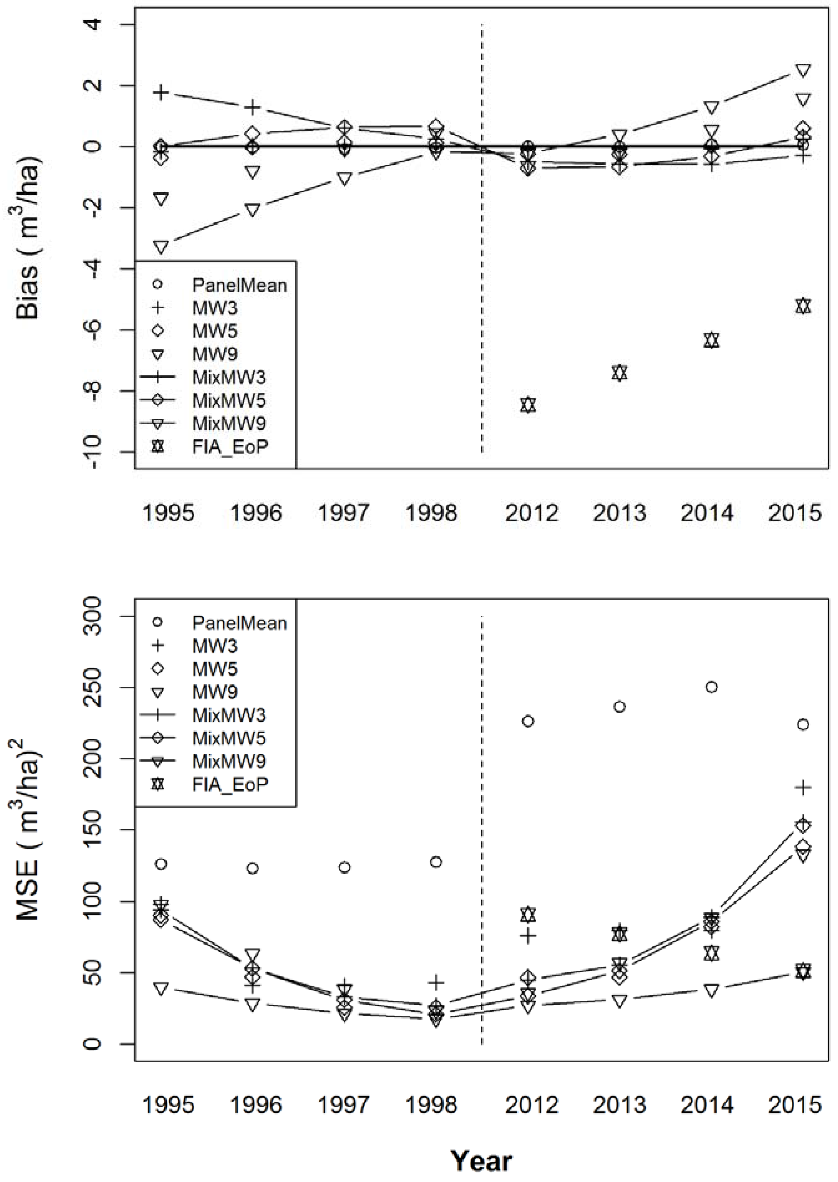
Figure 2 gives the results for the estimators for the first four and final four years, supplemented as described above. Note that the extrapolated or supplemented estimates are affected by two types of error; the first is the error in the most extraneous value of the non-supplemented estimator chain, and the second is the error based on the extent to which successive change differs from the estimated change in the outermost change interval. These errors combine to contribute to the increasing bias seen in Figure 2 for the supplemented estimators. The greatest bias is still observed in FIA_EoP, however, that estimator’s variance is low enough for its MSE to be tied with the MSE for the supplemented estimate from MixMW9 for the year 2015, the final year of the simulation, and the year that arguably might be of the greatest interest. All of the modeled estimators show lower MSEs than the panel mean for all of the years.
4. Discussion and Conclusions
Box [9] gave the admonition that “All models are wrong but some are useful.” He made the point that the question was not whether or not a model is “true,” because no model is “true” in every respect. What is needed are models that are useful and provide insight. Therefore, it is appropriate to judge estimators on the degree to which they achieve these goals. For the purpose of monitoring forest populations, it is useful to know what the current state of the population is, and how it has been changing, so that we can anticipate how it is likely to change in the future. If one keeps this in mind during the evaluation of the statistical properties of estimators, it will usually help lead one to a better decision in the choice of a model.
All of the estimators investigated here showed lower MSEs for the annual estimates than those achieved by using the “local” or single panel annual estimator, by allowing the use of a model to relate the year of interest to its neighboring years. The top graph of Figure 1 shows one thing clearly; in the simulation, FIA_EoP does possess the often noted lag-bias property (Van Deusen [10], Bechtold and Patterson [1] (p. 72)), while the other estimators do not. The graph also seems to show that as time progresses, the amount of lag bias decreases, while the bottom graph of Figure 1 shows a dramatic decrease in MSE for that estimator over the same period. However, given the model underlying FIA_EoP, it is instructive to note that the rate of change in the population is also decreasing over the range of estimates being made by FIA_EoP. That underlying model assumes that there has been no change in the variable over the number of years included in the estimator. Given that we know that there has been change in this variable over the years incorporated into each estimate produced by this estimator, this is an example of how this model is “false” or not true. However, as mentioned above, the pertinent questions are, “Is the model useful?” and “Does it provide insight?” To that end, note that it does provide insight into the general population trend, if the temporal lag is adjusted for in the model. If the trend is linear, then the temporal lag is exactly half of the cycle length. In the case of a 10-panel design, the FIA_EoP estimator simply becomes a MW10 if one assumes that the estimate of FIA_EoP is actually half of a cycle length earlier than it is. This can be seen by shifting the results for FIA_EoP in the top graph of Figure 1 to the left by five years. In this respect, one might argue that the estimator’s results, if kept in the proper perspective, can be useful and insightful. The dramatic decrease in MSE for the FIA_EoP estimator as time progresses would be a strong argument for the use of that estimator, if, in fact, we could always expect the estimator to continuously improve. However, as noted above, we have no reason to expect that. The moving window and dual-filter estimators have consistently low bias and MSE.
If we assume that the estimation of each year in the series is as important as any other year in the series, then we might assume our lowest risk or average loss would be achieved by the estimator that provides the lowest average annual MSE. In this simulation, examination of Figure 1 and Figure 2 together shows that this is achieved by the supplemented version of the dual-filter estimator MixMW9. The next best estimator by that criterion would be the supplemented version of MW9. Not long ago a decision between the use of MW9 and MixMW9 might have be made in favor of the former due to its simplicity and reduced use of computer resources. However, computer processing speeds have increased to the point to which the additional computations are no longer a serious impediment to the goal of achieving better estimates. As mentioned in the introduction, the estimators used in an NFI usually run within processes that often are not constantly monitored, which might still throw the argument in favor of the simpler estimator. Note, however, that although the MixMWx estimators might appear to be somewhat more complex, they ran quite successfully and uninterrupted in this simulation over 152 diverse populations. Additionally, the resources expended to obtain the data in an NFI in the first place always far outweigh the resources expended to process and analyze those data.
Acknowledgments
The author was funded by the United States government. The seed data for the simulations were collected through funding provided by the United States Department of Agriculture’s Forest Service, Forest Inventory and Analysis Program.
Conflicts of Interest
The author declares no conflict of interest.
Appendix A

Table A1.
Estimation units associated with the following USDA Forest Service’s FIA State Codes used to build the populations, given as State or Territory and Number of Units.
Table A1.
Estimation units associated with the following USDA Forest Service’s FIA State Codes used to build the populations, given as State or Territory and Number of Units.
| FIA State Code | Number of Units |
|---|---|
| AL | 6 |
| AR | 5 |
| CA | 6 |
| CT | 1 |
| DE | 1 |
| FL | 4 |
| GA | 5 |
| IL | 3 |
| IN | 4 |
| IA | 4 |
| KS | 3 |
| KY | 7 |
| LA | 5 |
| ME | 9 |
| MD | 4 |
| MA | 1 |
| MI | 4 |
| MN | 4 |
| MO | 5 |
| NE | 2 |
| NH | 2 |
| NJ | 1 |
| NY | 8 |
| NC | 4 |
| ND | 1 |
| OH | 6 |
| OR | 5 |
| PA | 6 |
| RI | 1 |
| SC | 3 |
| SD | 2 |
| TN | 5 |
| TX | 2 |
| VT | 2 |
| VA | 5 |
| WA | 5 |
| WV | 3 |
| WI | 5 |
| PR | 3 |
References
- Bechtold, W.A.; Patterson, P.L. (Eds.) The Enhanced Forest Inventory and Analysis Program-National Sampling Design and Estimation Procedures; Gen. Tech. Rep. SRS-80; U.S. Department of Agriculture Forest Service, Southern Research Station: Asheville, NC, USA, 2005. Available online: http://www.srs.fs.fed.us/pubs/20371 (accessed on 24 May 2017).
- Theil, H. On the use of incomplete prior information in regression analysis. J. Am. Stat. Assoc. 1963, 58, 401–414. [Google Scholar] [CrossRef]
- Van Deusen, P.C. Incorporating predictions into an annual forest inventory. Can. J. For. Res. 1996, 26, 1709–1713. [Google Scholar] [CrossRef]
- Van Deusen, P.C. Modeling trends with annual survey data. Can. J. For. Res. 1999, 29, 1824–1828. [Google Scholar] [CrossRef]
- Roesch, F. Spatial-Temporal Models for Improved County-Level Annual Estimates. In 2008 Forest Inventory and Analysis (FIA) Symposium, Proceedings of the RMRS-P-56CD, Park City, UT, USA, 21–23 October 2008; McWilliams, W., Moisen, G., Czaplewski, R., Eds.; comps. 2009; Department of Agriculture, Forest Service, Rocky Mountain Research Station: Fort Collins, CO, USA, 2009. [Google Scholar]
- Roesch, F.A. A simulation of Image-Assisted Forest Monitoring for National Inventories. Forests 2016, 7, 204. Available online: https://www.mdpi.com/1999-4907/7/9/204/htm (accessed on 31 May 2017). [CrossRef]
- Roesch, F.A.; Coulston, J.W.; Van Deusen, P.C.; Podlaski, R. Evaluation of Image-Assisted Forest Monitoring: A Simulation. Forests 2015, 6, 2897–2917. Available online: https://www.mdpi.com/1999-4907/6/9/2897/htm (accessed on 31 May 2017). [CrossRef]
- Roesch, F.A. Toward robust estimation of the components of forest population change. For. Sci. 2014, 60, 1029–1049. [Google Scholar] [CrossRef]
- Box, G.E.P. Robustness in the strategy of scientific model building. In Army Research Office Workshop on Robustness in Statistics, 11–12 April 1978; No. MRC-TSR-1954; Research Triangle Park: Durham, NC, USA, 1979; WISCONSIN UNIV-MADISON MATHEMATICS RESEARCH CENTER, 1979. [Google Scholar]
- Van Deusen, P.C. An Alternative View of Some FIA Sample Design and Analysis Issues. In Gen. Tech. Rep. NC-252, Proceedings of the Fourth Annual Forest Inventory and Analysis Symposium, New Orleans, LA, USA, 19–21 November 2002; McRoberts, R.E., Reams, G.A., Van Deusen, P.C., McWilliams, W.H., Cieszewski, C.J., Eds.; U.S. Department of Agriculture, Forest Service, North Central Research Station: St. Paul, MN, USA, 2005; 258p. [Google Scholar]
Figure 1.
The weighted means relative to the weighted true means of initial volume (the volume at the beginning of each year) over the 152 populations (top) and weighted mean squared errors (bottom) for the eight volume estimators including the annual Panel Mean, FIA_EoP, MW3, MW5, MW9, MixMW3, MixMW5, and MixMW9.

Figure 2.
The weighted bias (top) and weighted mean squared errors (bottom) of eight volume estimators supplemented by linear extrapolation.
Figure 2.
The weighted bias (top) and weighted mean squared errors (bottom) of eight volume estimators supplemented by linear extrapolation.
© 2017 by the author. Licensee MDPI, Basel, Switzerland. This article is an open access article distributed under the terms and conditions of the Creative Commons Attribution (CC BY) license (http://creativecommons.org/licenses/by/4.0/).
Share and Cite
MDPI and ACS Style
Roesch, F.A. Dual-Filter Estimation for Rotating-Panel Sample Designs. Forests 2017, 8, 192. https://doi.org/10.3390/f8060192
AMA Style
Roesch FA. Dual-Filter Estimation for Rotating-Panel Sample Designs. Forests. 2017; 8(6):192. https://doi.org/10.3390/f8060192
Chicago/Turabian StyleRoesch, Francis A. 2017. "Dual-Filter Estimation for Rotating-Panel Sample Designs" Forests 8, no. 6: 192. https://doi.org/10.3390/f8060192
Note that from the first issue of 2016, this journal uses article numbers instead of page numbers. See further details here.