How Similar Are Forest Disturbance Maps Derived from Different Landsat Time Series Algorithms?

Abstract

Disturbance is a critical ecological process in forested systems, and disturbance maps are important for understanding forest dynamics. Landsat data are a key remote sensing dataset for monitoring forest disturbance and there recently has been major growth in the development of disturbance mapping algorithms. Many of these algorithms take advantage of the high temporal data volume to mine subtle signals in Landsat time series, but as those signals become subtler, they are more likely to be mixed with noise in Landsat data. This study examines the similarity among seven different algorithms in their ability to map the full range of magnitudes of forest disturbance over six different Landsat scenes distributed across the conterminous US. The maps agreed very well in terms of the amount of undisturbed forest over time; however, for the ~30% of forest mapped as disturbed in a given year by at least one algorithm, there was little agreement about which pixels were affected. Algorithms that targeted higher-magnitude disturbances exhibited higher omission errors but lower commission errors than those targeting a broader range of disturbance magnitudes. These results suggest that a user of any given forest disturbance map should understand the map’s strengths and weaknesses (in terms of omission and commission error rates), with respect to the disturbance targets of interest.

1. Introduction

Forest ecosystems are strongly influenced by disturbance processes that interact with the climate and other environmental factors to alter their state and function. For example, in Europe, increases in insect, wind, and fire disturbances, first noted in the 20th century, have continued into the 21st century and are thought to be strong contributors to a recently observed saturation of the forest carbon sink [1]. Disturbances can range from high-impact, discrete events (such as fires, windstorms, and deforestation, all of which dramatically and sometimes permanently alter forest conditions [2]) to subtler and often gradual and chronic processes that require many years to unfold (such as prolonged droughts that result in partial reduction in canopy cover and increased insect activity [3,4]). Although high-impact disturbances can have immediate and profound effects on forest function, especially locally, they are generally far less common than subtler disturbances that accumulate over time and space, often having significant aggregate effects on forest function [5,6]. In the context of this inclusive description of forest disturbance, the goal of this study is to explore the ability of seven different remote sensing algorithms to map forest disturbance and the consistency among the algorithms in doing so.

Remote sensing has long played an important role in characterizing forest disturbance [7], and systematically collected, global remote sensing datasets are key to emerging forest monitoring programs [3,8]. Forest disturbance monitoring benefits greatly from retrospective analyses, as these help establish historic relationships between human (e.g., land use, forest policy and management) and natural (e.g., fire, wind, insects and disease) disturbance drivers, disturbance patterns, and post-disturbance recovery or resilience dynamics [9]. Data from the Moderate Resolution Imging Spectrometer (MODIS) sensors have played an important role in forest monitoring during the 21st century [10], but the relatively coarse spatial resolution of these data precludes the detection of the myriad of small and subtle disturbances that are so prevalent across the Earth’s forests [3,11]. Landsat, with an over-40-year global record of near-30-m resolution data, is thus far the best remote sensing option for resolving the full range of disturbance occurrences [6,12].

Over the past several years there have been significant advances in disturbance mapping algorithms that use Landsat data [13], taking advantage of the high-quality data archive that became freely available in 2008 [14]. Users of forest disturbance maps now have a palette of new products becoming available to choose from and they need to understand which are best suited to their needs. In this study, we examine seven specific algorithms that push the frontier of forest disturbance mapping by utilizing unprecedented numbers of Landsat images. As such, these algorithms perform high temporal density analyses that have the potential to yield improved temporally and spatially detailed disturbance maps. Below, we summarize the salient differences among these algorithms; for detailed specifications of the individual algorithms, refer to the algorithms’ source citations listed in

Table 1. Algorithms used to derive forest disturbance map products evaluated in this study. See citations for greater detail.

Algorithm	Citations	Disturbance Target Population	Bands/Indices, This Study	Basic Approach
LandTrendr (Landsat-based detection of Trends in Disturbance and Recovery)	[15]	Discrete events and gradual trends; broad range of disturbance magnitudes; forests only	NBR	Temporal segmentation of annual series; pixel as analysis unit
ITRA (Image Trends from Regression Analysis)	[16]	Gradual trends; broad range disturbance magnitudes; all woody vegetation	NDVI	Slope of annual series over multi-year epochs; pixel as analysis unit
VCT (Vegetation Change Tracker)	[17]	Discrete events; limited range of disturbance magnitudes; forests only	Forestness Index	Multi-year departure of annual series from previous year; pixel as analysis unit
EWMACD (Exponentially Weighted Moving Average Change Detection)	[5]	Discrete events; broad range of disturbance magnitudes; forests only	NDVI	Multi-year departure from phenology model based on every clear observation from previous years; pixel as analysis unit
MIICA (Multi-index Integrated Change Analysis)	[18]	Discrete events; limited range of disturbance magnitudes; all land cover types	NBR, NDVI, Change Vector, Relative Change Vector	Bi-temporal differencing of annual series; pixel as analysis unit
CCDC (Continuous Change Detection and Classification)	[19,20]	Discrete events; limited range of disturbance magnitudes; all land cover types	Bands 2–5, 7	Multi-year departure from phenology model based on every clear observation from previous years; pixel as analysis unit
VeRDET (Vegetation Regeneration and Disturbance Estimates Through Time)	[21]	Discrete events and gradual trends; broad range of disturbance magnitudes; forests only	NDMI	Temporal segmentation of annual series; pixel as analysis unit (after initial spatial segmentation)

.

Generally, the algorithms used here differ in their specificity with respect to target populations (Table 1), detecting discrete, gradual (i.e., trends) or both types of disturbances, having different sensitivities to disturbance magnitudes based on thresholding, and by limiting analyses to different land cover types. Those that focused exclusively on forests either targeted a broad range of disturbance magnitudes (LandTrendr, Landsat-based detection of Trends in Disturbance and Recovery; EWMACD, Exponentially Weighted Moving Average Change Detection; VeRDET, Vegetation Regeneration and Disturbance Estimates Through Time) or a more limited range of magnitudes (VCT, Vegetation Change Tracker). One algorithm targeted a broad range of disturbance magnitudes across forest, woodland, and shrub communities (ITRA, Image Trends from Regression Analysis). The others focused on disturbance across all land cover types, but targeted a more limited range of magnitudes (MIICA, Multi-index Integrated Change Analysis; CCDC, Continuous Change Detection and Classification). LandTrendr and VeRDET targeted both discrete events and gradual trends, whereas ITRA targeted only gradual trends, and VCT, EWMACD, MIICA, and CCDC targeted only discrete events.

The algorithms varied in terms of how the spectral, spatial, and temporal domains were exploited. Most used a single spectral band or index (LandTrendr, ITRA, VCT, EWMACD, VeRDET), while others used multiple bands or indices (MIICA, CCDC), and all used the pixel as the unit of analysis (although VeRDET used pre-defined polygons for spectral smoothing, and VCT defined a forest norming population based on image statistics [17]). Most algorithms used a single spectral observation per year to construct an annual time series, whereas EWMACD and CCDC used every clear observation for all years to derive a phenology model. LandTrendr and VeRDET used a temporal segmentation to define disturbances, ITRA calculated slopes of spectral trends across specific temporal epochs, VCT sought multi-year departures from the previous years’ values, MIICA used bi-temporal differencing, and EWMACD and CCDC sought multi-year departures from modeled expectations.

Maps from each of the seven individual algorithms evaluated here have been independently evaluated for quality and all performed well when compared against unique reference datasets representing their different target populations (see citations in Table 1). However, to date, there have been no independent and in-depth inter-comparative analyses of disturbance map products derived from these algorithms, many of which are pushing the magnitude boundaries of disturbance detection. Comparative analyses are important so that potential users understand the limitations and relevance of these products for specific applications.

Some interesting and important general questions arise in the context of in-depth comparative analyses among disturbance map products: How much agreement is there among the forest disturbance maps derived from these algorithms? Is agreement a function of spectral change magnitude associated with apparent disturbances? How sensitive are the algorithms to the spectral change magnitudes associated with a full range of disturbance severities? With these broad questions in mind, we addressed the following specific questions:

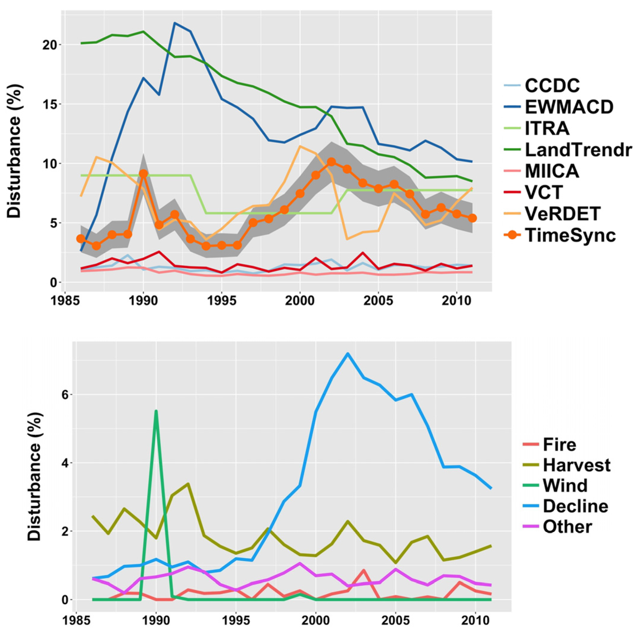
• How do the map products derived from the seven algorithms (Table 1) agree in terms of aggregate area disturbed over six Landsat scenes distributed across diverse forested regions of the conterminous US? Similarly, how do these compare with disturbance area estimates determined from an independent probability sample where disturbance was identified by human interpretation using the TimeSync-based methodology [22]?
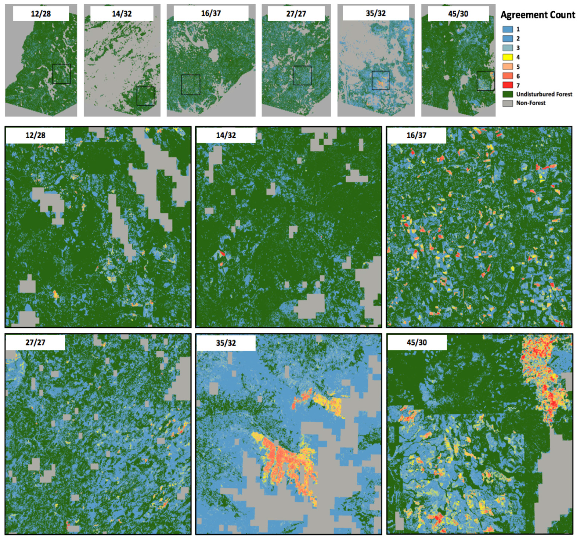
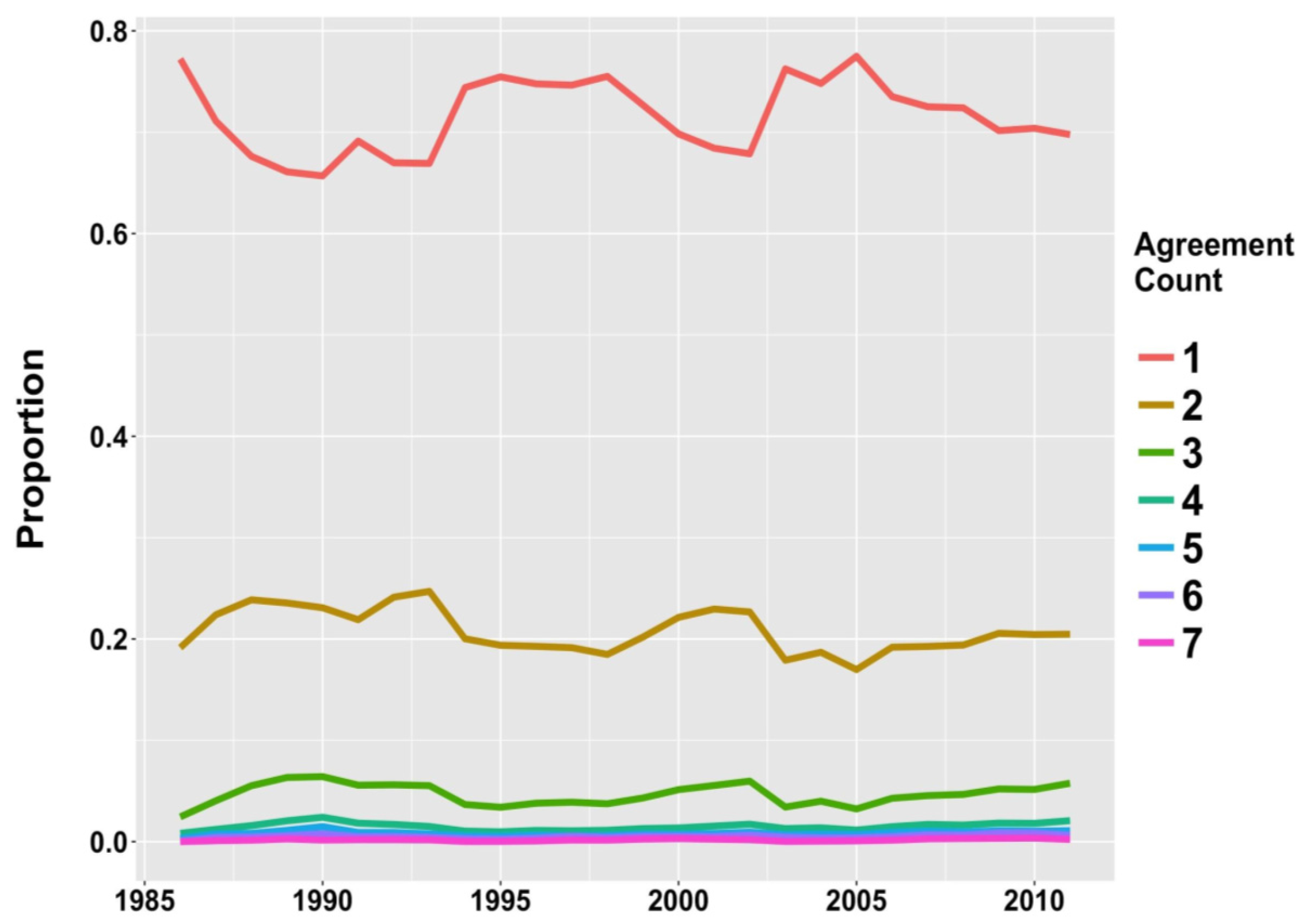
• How much agreement is there at the pixel level among the map products in their spatial depictions of forest disturbance over time?
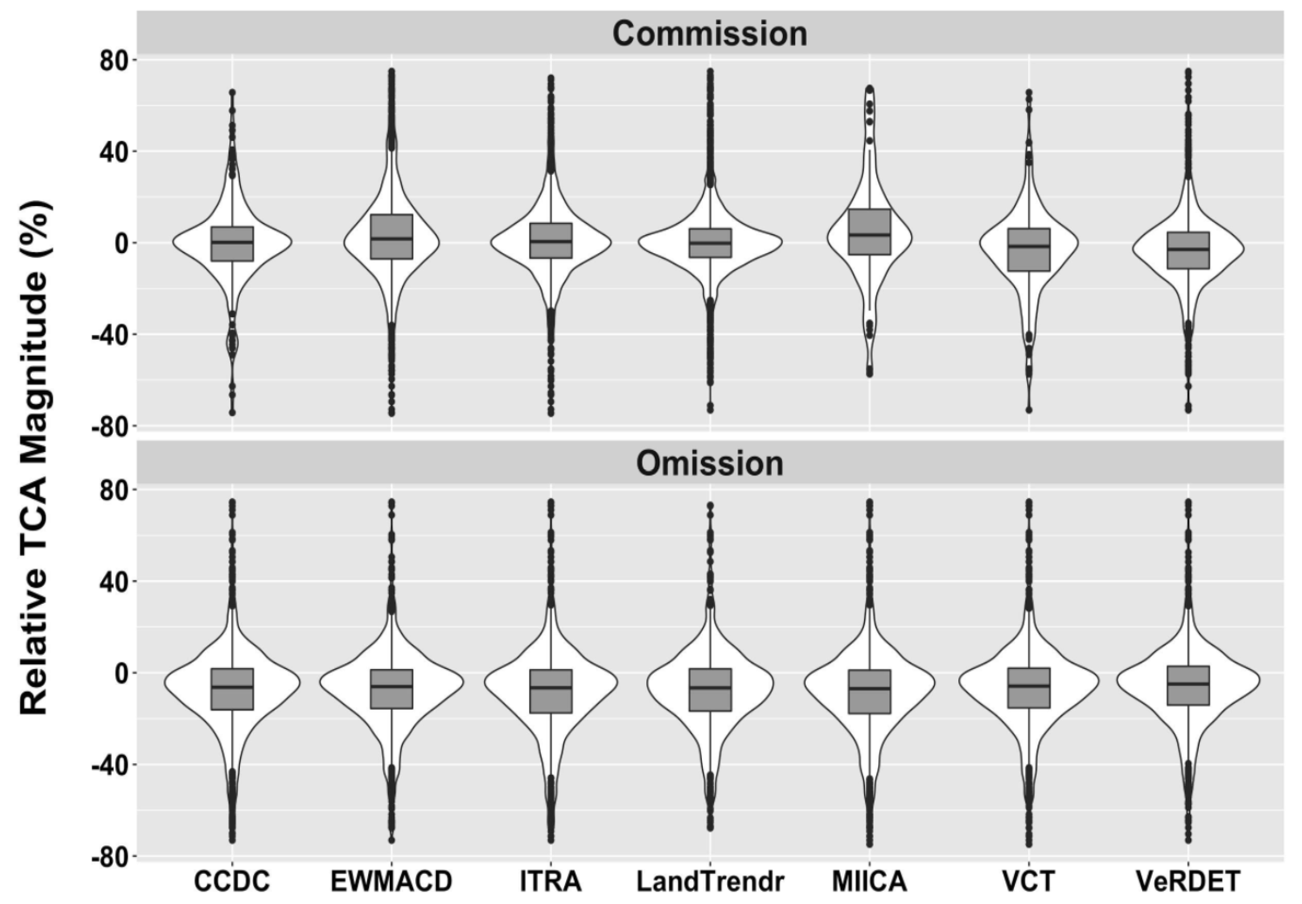
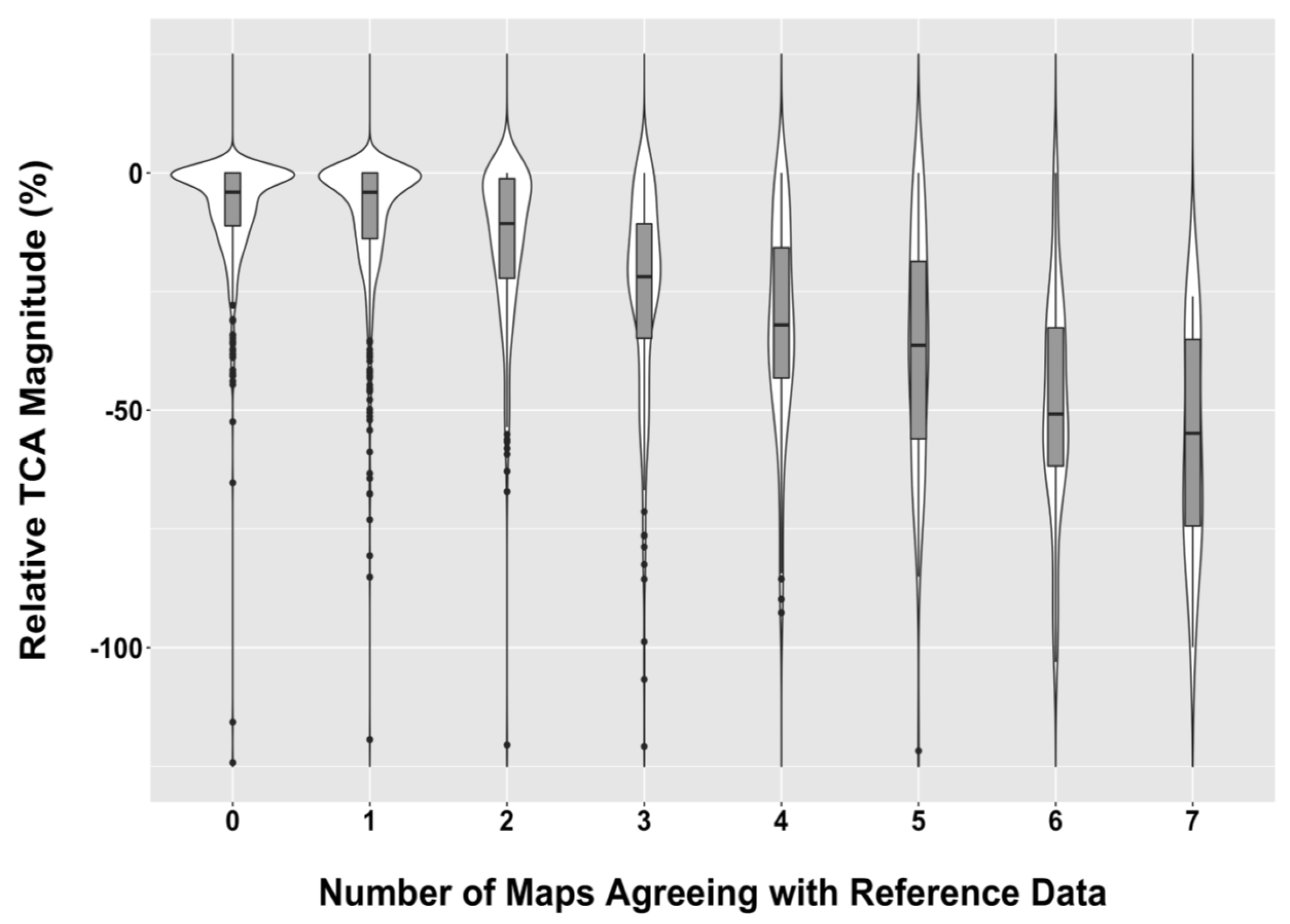
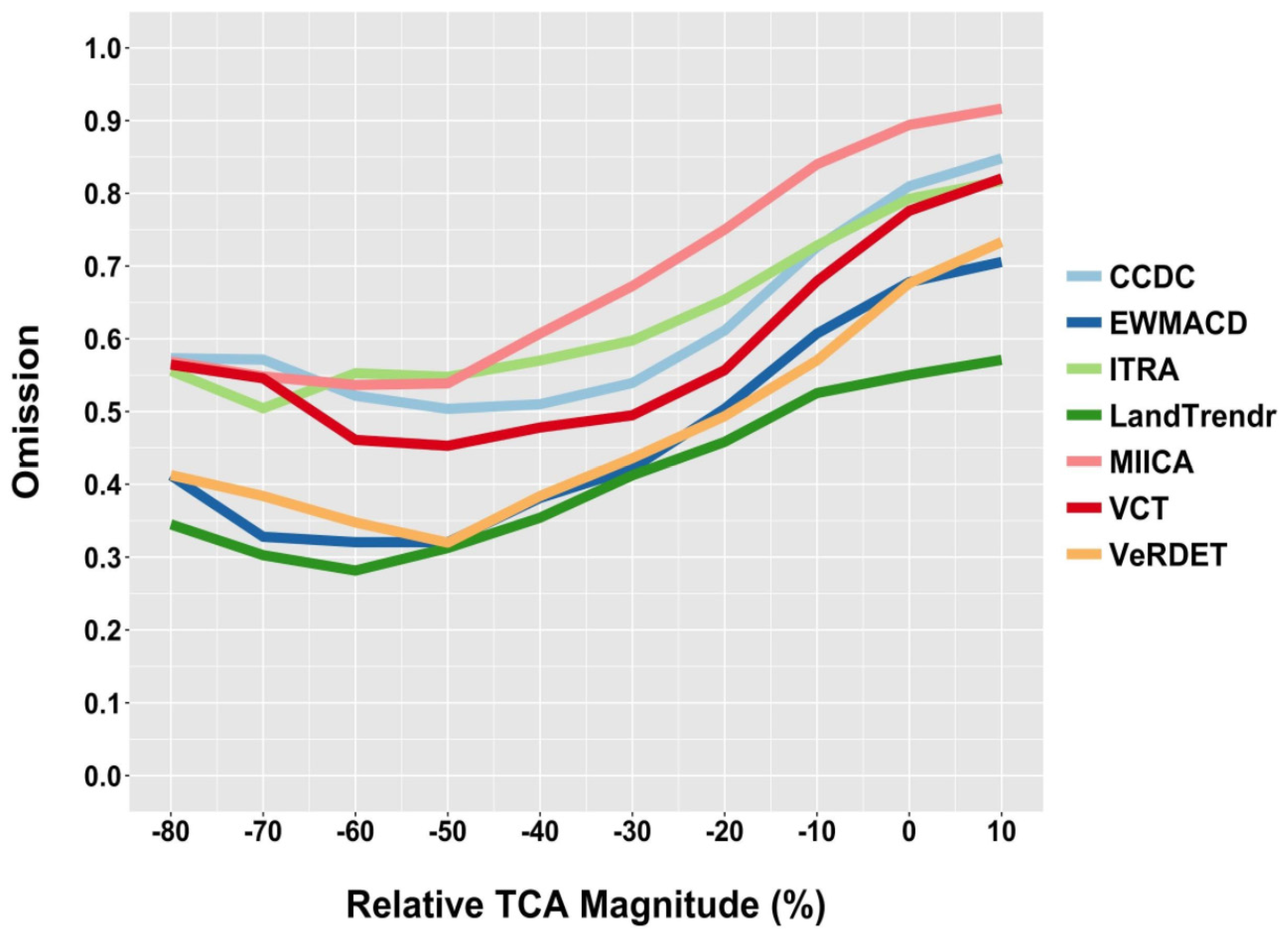
• Compared to a reference dataset, how do mapped disturbance omission and commission differ among the map products, and how closely related are these to the spectral change magnitude?

2. Materials and Methods

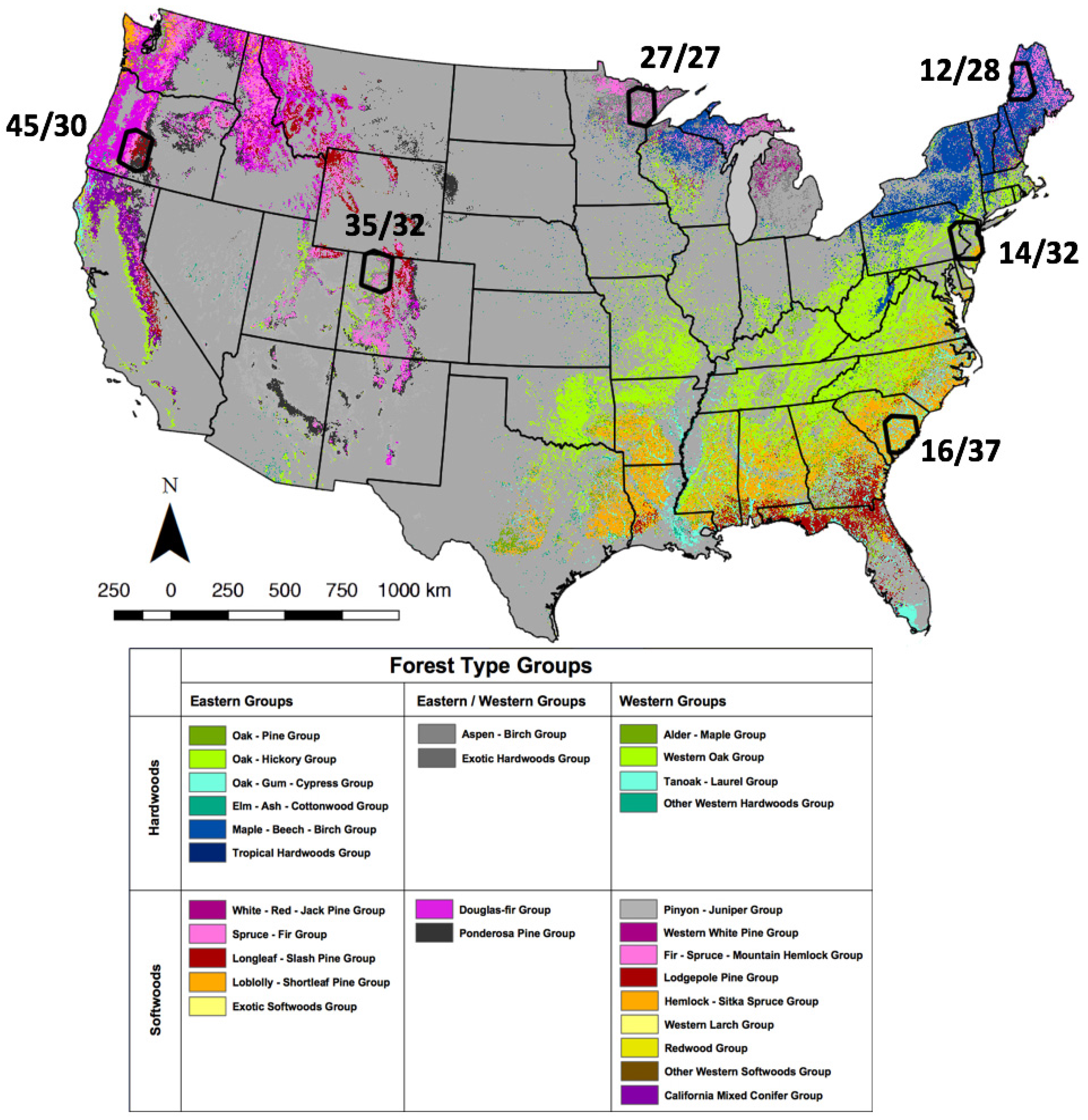
2.1. Study Scenes

Six areas widely dispersed across the conterminous US were the focus of this study (Figure 1). These areas were defined as the non-overlapping portions of six individual, Landsat frames, known as TSAs (Thiessen Scene Areas; [15]), from the second World Reference System (WRS-2) grid. The six scenes (given by numeric WRS-2 Path/Row) included: 12/28 in northern Maine; 14/32 in eastern Pennsylvania and New Jersey; 16/37 in coastal South Carolina; 27/27 in northern Minnesota; 35/32 in northwestern Colorado; and 45/30 in western Oregon. The Canadian portion of scene 12/28 was excluded from the study, as was the significant section of the Atlantic Ocean in 16/37. These scenes were selected to represent a wide range of forest ecosystems, which ensured that a diversity of forest type groups (

Table 2. Area of forest type groups in each Landsat scene (Path/Row). Data from [24].

	Area (ha) per Landsat Path/Row
Forest Type Group	12/28	14/32	16/37	27/27	35/32	45/30	Total
White/Red/Jack Pine Group	644	94	0	35,288	0	0	36,025
Spruce/Fir Group	661,588	19	0	430,213	0	0	1,091,819
Longleaf/Slash Pine Group	0	0	5631	0	0	0	5631
Loblolly/Shortleaf Pine Group	0	163,956	1,069,100	0	0	0	1,233,056
Pinyon/Juniper Group	0	6600	0	0	168,969	8131	183,700
Douglas-fir Group	0	0	0	0	2388	445,938	448,325
Ponderosa Pine Group	0	0	0	0	3119	597,481	600,600
Western White Pine Group	0	0	0	0	0	388	388
Fir/Spruce/Mountain Hemlock Group	0	0	0	0	267,994	401,731	669,725
Lodgepole Pine Group	0	0	0	0	82,356	367,031	449,388
Hemlock/Sitka Spruce Group	0	0	0	0	0	350	350
Other Western Softwood Group	0	0	0	0	94	75	169
California Mixed Conifer Group	0	0	0	0	0	631	631
Exotic Softwoods Group	0	38	0	0	0	0	38
Oak/Pine Group	0	14,231	37,681	38	0	0	51,950
Oak/Hickory Group	0	408,519	41,188	256	0	0	449,963
Oak/Gum/Cypress Group	0	10,625	454,731	0	0	0	465,356
Elm/Ash/Cottonwood Group	81	14,506	10,606	9356	1056	0	35,606
Maple/Beech/Birch Group	673,650	37,350	0	14,581	0	0	725,581
Aspen/Birch Group	24,188	925	0	1,023,113	359,781	231	1,408,238
Alder/Maple Group	0	0	0	0	0	6	6
Western Oak Group	0	0	0	0	120,150	369	120,519
Tanoak/Laurel Group	0	0	0	0	0	19	19
Other Western Hardwoods Group	0	0	0	0	100	0	100
Total Forest Area	1,360,150	656,863	1,618,938	1,512,844	1,006,006	1,822,381	7,977,181
Total Non-Forest Area	121,700	1,407,844	314,000	287,844	1,074,863	164,625	3,370,876
Total Scene Area	1,481,850	2,064,706	1,932,938	1,800,688	2,080,869	1,987,006	11,348,056
Percent Forest	91.8	31.8	83.8	84.0	48.3	91.7	70.3

) and forest change processes (e.g., harvest, fire, insects, and urbanization as depicted in Figure 5 of [23]) were available for comparing map products.

2.2. Landsat Images, Synthetic Images, and Map Products

All map products were based on a common stack of Landsat time series images for each of the six scenes. To construct the stacks, all available TM and ETM+ images (1984–2012) in standard L1T format were downloaded from the archive, after derivation of surface reflectance using LEDAPS [25,26]. Accompanying each image was a LEDAPS-derived cloud mask, and an additional cloud mask derived for each image with Fmask [27]. For map production, two algorithms used all clear pixels from all available images (CCDC, EWMACD) and three used annual image composites with a target date of August 6, based on algorithm-specific techniques (LandTrendr, VCT, VeRDET; see citations, Table 1). Two algorithms (ITRA, MIICA) used synthetic images generated from all available data in L1T stacks, based on the time series model components of the CCDC algorithm [19,20], which is similar to the harmonic regression basis of EWMACD [5]. The time series model incorporated the seasonality, trend, and breaks contained in every clear pixel of the Landsat time series for each spectral band. The predicted images used in this study were for August 6th of every year.

The L1T image stacks and synthetic data were distributed among the algorithm developers, who each ran their respective algorithms on the selected datasets described above and returned basic algorithm output (see citations in Table 1) to a central location. Basic output included, depending on algorithm, multiple discrete disturbances at different times over the time series, and/or multiple consecutive years of change commonly associated with gradual disturbance. To compare the maps on a common basis, we extracted information identifying where and for what years disturbances were detected. For gradual disturbances, all years where consecutive disturbance was identified were included. We then created an annual set of binary time series disturbance maps, labeling all mapped pixels as disturbed or not disturbed for each year. The first two (1984, 1985) and last (2012) years of imagery were used by all algorithms, but as these bounded the time series they were generally unreliable for disturbance detection. Thus, each disturbance map set (one per algorithm) for each scene started with 1986 and ended with 2011. The forest type group map from [24] was used to trim all map sets for each scene to a common forest mask before comparison.

2.3. Reference Data

The TimeSync Landsat time series visualization and change data collection tool [22] was used to collect change reference data for this study. TimeSync enabled accurate disturbance characterizations for pixel-level samples of Landsat time series data, relying on human interpretations of change as viewed in image chip series, spectral index trajectories, high spatial resolution image temporal snapshots from Google Earth, and other ancillary disturbance products. TimeSync and similar approaches have been used or recommended in a variety of settings [6,9,15,28,29,30,31] and the interested reader is directed there for more detailed descriptions of the system and its potential usage.

Within each scene, 300 pixels were selected using simple random sampling, without respect to land cover. Each sampled pixel was interpreted for forest disturbance occurrence, noting for each occurrence the first year of detection (a year between 1986 and 2011), the duration for gradual disturbances (in number of years), and the causal agent class (harvest, fire, decline, wind, other). Disturbance spectral change magnitude was calculated using the Tasseled Cap angle (TCA) index [32], in relative terms, as the difference between the pre-disturbance and post-disturbance TCA values divided by the pre-disturbance value [6]. Dividing this result by duration yielded a relative TCA change per year for each disturbance occurrence. A total of 1303 of the 1800 (300 per scene) sample pixels were forested at some point within the 26-year time period of observation (as determined with TimeSync) and were included in this analysis, yielding 33,878 total observations (1 observation per year per sampled pixel).

2.4. Aggregate Disturbance Rates (Question 1)

Aggregate disturbance rates, across all mapped pixels of all six scenes, were derived from each algorithm’s annual binary disturbance map set. This involved, for each year, summing the area of all disturbed forested pixels across scenes and dividing by the total area of forest in the six scenes (Table 2). To compare the algorithm map products, we plotted the results as annual time series of disturbance rates (proportion of forest area disturbed) for the six-scene collection from each algorithm’s disturbance map sets. For comparison with the map-based forest disturbance rates, sample-based TimeSync forest disturbance rate estimates were plotted on the same graph (with 95% confidence intervals). For the formulas below, the condition of the pixel as being forest or not was determined from the reference sample. Likewise, the total forest area for the six scenes was not known (i.e., the forest type map of [24] was not used here), but was estimated from the sample, creating the need for the ratio estimator below. Note that the forest area derived from the Reufenacht et al. [24] mask (Table 2) used to compare the disturbance map products and the forest area derived from the samples below will be different; but those differences are expected to be small relative to differences in mapped and estimated disturbance rates. This is because the correspondence between the forest mask and TimeSync samples regarding forest versus non-forest was high (i.e., 93%).

To calculate sample-based annual disturbance rate estimates for our population of six scenes, each scene was considered a stratum, and the inclusion probability for a pixel was n_h/N_h, where N_h = number of US land (i.e., non-ocean) pixels in scene h and n_h = 300 is the sample size in each stratum. The proportion of forest area disturbed was estimated as a ratio R = Y/X, where Y is the population total of y_u,

$${\mathit{y}}_{\mathit{u}}=\{\begin{array}{c}1 \mathit{i}\mathit{f} \mathit{p}\mathit{i}\mathit{x}\mathit{e}\mathit{l} \mathit{u} \mathit{i}\mathit{s} \mathit{d}\mathit{i}\mathit{s}\mathit{t}\mathit{u}\mathit{r}\mathit{b}\mathit{e}\mathit{d}\\ 0 \mathit{i}\mathit{f} \mathit{p}\mathit{i}\mathit{x}\mathit{e}\mathit{l} \mathit{u} \mathit{i}\mathit{s} \mathit{n}\mathit{o}\mathit{t} \mathit{d}\mathit{i}\mathit{s}\mathit{t}\mathit{u}\mathit{r}\mathit{b}\mathit{e}\mathit{d}\end{array}$$

(1)

and X is the population total of x_u,

$${\mathit{x}}_{\mathit{u}}=\{\begin{array}{c}1 \mathit{i}\mathit{f} \mathit{p}\mathit{i}\mathit{x}\mathit{e}\mathit{l} \mathit{u} \mathit{i}\mathit{s} \mathit{f}\mathit{o}\mathit{r}\mathit{e}\mathit{s}\mathit{t}\\ 0 \mathit{i}\mathit{f} \mathit{p}\mathit{i}\mathit{x}\mathit{e}\mathit{l} \mathit{u} \mathit{i}\mathit{s} \mathit{n}\mathit{o}\mathit{t} \mathit{f}\mathit{o}\mathit{r}\mathit{e}\mathit{s}\mathit{t}\end{array}$$

(2)

The parameter R is the total area disturbed divided by the total area of forest (or equivalently, the total number of pixels disturbed divided by the total number of forest pixels). The combined ratio estimator denoted $\widehat{R}$ [33] (Section 6.11), was used to estimate R for the stratified random sample (each of the six scenes being a stratum),

$$\widehat{\mathit{R}}=\frac{{\sum }_{h=1}^6{N}_h{\overline{y}}_h}{{\sum }_{h=1}^6{N}_h{\overline{x}}_h}$$

(3)

where ${\overline{x}}_h$ is the sample mean of $x_u$ in stratum h and ${\overline{y}}_h$ is the sample mean of $y_u$ in stratum h. The estimated variance of the combined ratio estimator is

$$\widehat{\mathit{V}}(\widehat{\mathit{R}})=\left(\frac{1}{{\widehat{\mathit{X}}}^2}\right)\left[{\sum }_{\mathit{h}=1}^{\mathit{H}}{\mathit{N}}_{\mathit{h}}^2 (1-{\mathit{n}}_{\mathit{h}}/{\mathit{N}}_{\mathit{h}})({\mathit{s}}_{\mathit{y}\mathit{h}}^2+{\widehat{\mathit{R}}}^2{\mathit{s}}_{\mathit{x}\mathit{h}}^2-2\widehat{\mathit{R}}{\mathit{s}}_{\mathit{x}\mathit{y}\mathit{h}}/{\mathit{n}}_{\mathit{h}})\right]$$

(4)

where $\widehat{X}$ is the denominator of $\widehat{R}$, $s_{yh}^2$ and $s_{xh}^2$ are the sample variances of $y_u$ and $x_u$ for stratum $h$, and $s_{xyh}$ is the sample covariance for $y_u$ and $x_u$ for stratum $h$.

2.5. Map-to-Map Agreement (Question 2)

Direct spatial comparison of the maps at the pixel level required overlaying the original algorithm disturbance map sets for each scene by year. For example, for 27/27, all seven maps for 1986 were extracted from the original map sets and overlaid in a single, new stack, a process that was repeated for each subsequent year. For each pixel, the number of maps having that pixel labeled as disturbance was determined for a given year and these counts were displayed as an agreement map. As a collection across years, for a given scene, these new maps are referred to as agreement map sets, where a given set represents annual series depicting the number of maps that declared a disturbance for each year at the pixel level. Counts varied from zero to seven, with the former meaning that no map declared a disturbance for a given pixel in a given year and the latter meaning that all maps declared a disturbance.

Once created, we summarized each agreement map set to derive annual series of disturbance counts. For each year, the summarization included: (i) calculating unanimous “no disturbance” (count equal to zero) in terms of proportion of total forest area per scene; (ii) calculating proportions of total forest area per scene for counts from one to seven; (iii) and relativizing the disturbance counts (from one to seven) by determining the proportion of total area mapped as disturbed represented by each non-zero count. Summing the relativized proportions of non-zero counts yields 1, accounting for all pixels mapped as disturbed by at least one algorithm at the scene level for each year. Because we might expect as much as one-year offset in timing of mapped disturbances given specific image dates chosen by algorithms that use a single growing season observation per year [22], we repeated the analysis declaring agreement when timing of mapped disturbances was within one year of each other among map sets.

2.6. Map-to-Reference Data Agreement (Question 3)

TimeSync reference data were compared against the original disturbance map sets at the sample pixel locations to quantify map omission and commission for each map set across scenes and time. This was based on the proportion of the total number of observations labeled as disturbed by TimeSync that were not labeled as disturbed by a given map set (omission) and the proportion of total number of observations labeled as disturbed by a given map set that were not labeled as disturbed by TimeSync (commission). This was done once for each original disturbance map set, yielding a pair of map omission and commission values for each map set that we rendered as a scatterplot. To allow for one-year offset, this analysis was repeated by declaring agreement when timing of mapped disturbances was within one year of TimeSync observed disturbance. The one-year offset analysis treated both commission and omission equally.

To examine the relationship between map error and spectral change magnitude we plotted distributions of relative TCA change derived from the TimeSync reference data for all omitted annual observations within the set of original disturbance maps. We repeated this for commission observations after first calculating relative TCA magnitudes for each committed observation from the TimeSync reference data.

3. Results

3.1. Aggregate Disturbance Rates (Question 1)

Across the six study scenes, aggregate disturbance rates derived from the disturbance map sets were highly variable over time, as expressed by the different algorithms and the reference data (Figure 2, top). Algorithms with the lowest mapped disturbance rates included those that targeted the more limited, higher-magnitude disturbances—MIICA, CCDC, and VCT, with across time average rates of 0.82%, 1.24%, and 1.42%, respectively. Those algorithms that targeted the broader range of disturbance magnitudes mapped higher disturbance rates. LandTrendr and EWMACD mapped the highest disturbance rates (cross-time averages of 15.24% and 12.77%, respectively), with the rates from VeRDET and ITRA being more moderate (6.74% and 7.52%, respectively). The latter two mapped disturbance rates closest to those from the reference samples (5.96% per year on average). It should be noted that map products excluding explicit capture of gradual disturbances (VCT, EWMACD, MIICA, and CCDC) might be penalized in this analysis where gradual disturbances were observed in the reference data. In some cases, where gradual disturbances reached (in a given year) a change threshold high enough for detection, these algorithms might have captured the disturbance as a one-year event, even though the reference data and other algorithms might have recorded a multi-year event. EWMACD was less likely to be effected in this way because it targeted a broader range of disturbance magnitudes and was able to represent several successive years of disturbance associated with gradual change.

3.2. Map-to-Map Agreement (Question 2)

As derived from the agreement map sets, there was agreement among all seven original disturbance map sets that the majority of the forest area was not disturbed in any given year. The percentage of forest area where no algorithm detected disturbance ranged from 60.3% (1992) to 74.8% (2009), with a mean of 67.4% (standard deviation of 4.3%) across time. The complement of that, 32.6%, is the average annual area mapped as disturbed by at least one algorithm. Not surprisingly, given the widely varying disturbance rates derived from the disturbance map sets, there was little correspondence at the pixel level in the map sets themselves (Figure 3). For example, in 27/27 most of the pixel-level disturbance for the year 2002 was mapped by just one algorithm, although the specific algorithm mapping disturbance is highly variable among pixels (data not shown).

Of the total amount of disturbance mapped across scenes in any given year, between 66% and 80% (mean of 71.5% across time) of disturbance was mapped by a single algorithm (Figure 4). On average, across time, 20.8% of all mapped disturbance was mapped by two algorithms and 4.7% was mapped by three algorithms at a time. The majority were in agreement about mapped disturbance only 3.0% of the time (1.5%, 0.8%, 0.5%, and 0.2% on average for four, five, six, and seven map sets, respectively). Allowing for a one-year offset between the maps generally improved the agreement, but only moderately, with (on average) well over 60% of all mapped disturbances still being mapped by only one algorithm in any given year.

3.3. Map-to-Reference Data Agreement (Question 3)

TimeSync reference data consisted of 988 unique observed disturbance occurrences (including gradual, multi-year disturbance occurrences) over time across the six study scenes. The largest proportion was harvest events (61.5%), followed by decline (17.9%), other (9.0%), wind (6.2%), and fire (5.4%). All fire and wind occurrences had a one-year duration, as did the vast majority of harvest occurrences. The class “other” had durations that were mostly one year (64%), with the large majority of the remaining occurrences having a duration of two years. Decline was unique, representing a largely gradual change class, with 54% of all occurrences having a duration of five or more years.

Disturbance occurrences had a broad range of TCA change magnitudes (Figure 5). The median values of per-occurrence relative TCA change for each agent class were −33.8% (fire), −22.1% (harvest), −21.9% (other), −12.0% (decline), −11.5% (wind), with an overall across-class value of −19.7%. Because decline was generally a gradual change process, annual change magnitudes for this class were closer to 2% per year. Across the six scenes, harvest was dominant in the first part of the time series until the late 1990s (except for 1990 when wind associated with Hurricane Hugo in 16/37 dominated), when decline (associated largely with tree mortality in 35/32 and 45/30) became the dominant disturbance agent (Figure 2, bottom). This result is similar to that from a recent national-level study [6], confirming that the six scenes used here are representative of national forest type and disturbance regimes.

Relative to TimeSync reference data, map omission ranged from 58.9% (LandTrendr) to 92.6% (MIICA) and commission from 36.5% (CCDC) to 85.3% (ITRA) among the map sets (Figure 6). Those algorithms that exhibited the lowest omission rates (LandTrendr, EWMACD, and VeRDET) also had the highest commission rates. Conversely, those that exhibited the lowest commission rates also had the highest omission rates (VCT, MIICA, and CCDC). ITRA had relatively high rates of both omission and commission. Allowing for a one-year offset between the maps and reference data reduced omission errors by 3% or less for most map products. Commission errors for three map sets were reduced more substantially, allowing for the one-year offset—8% for MIICA, 11% for VCT, and 15% for CCDC—with all other map sets benefitting from commission reductions of 1.4% or less.

The relative TCA change magnitudes among map sets for omitted disturbances were generally quite small, with median values ranging between −5.0% (VeRDET) and −7.0% (MIICA) (Figure 7, bottom). Similarly, the magnitudes for committed disturbances were also quite low, with median values ranging from −3.7% (CCDC) to 4.0% (MIICA) (Figure 7, top). The map omission by reference data disturbance agent class indicates that the agent classes with the highest TCA change magnitudes (fire and harvest, Figure 5) were associated with the lowest omission rates (

Table 3. Map omission by TimeSync disturbance causal agent class.

	Harvest		Fire		Decline		Wind		Other
Map	Omission (%)	Standard Error (%)	Omission (%)	Standard Error (%)	Omission (%)	Standard Error (%)	Omission (%)	Standard Error (%)	Omission (%)	Standard Error (%)
CCDC	63.6	2.7	66.5	6.1	98.2	0.3	86.9	0.6	83.1	4.9
EWMACD	59.9	7.2	53.7	7.4	80.4	6.1	57.3	2.0	60.2	10.6
ITRA	68.8	7.1	62.8	12.8	93.0	2.5	85.2	0.7	64.9	6.6
LandTrendr	53.3	1.2	40.7	4.2	58.7	6.2	70.4	1.4	61.3	8.2
MIICA	82.0	3.2	66.5	13.0	99.5	0.2	96.7	0.2	84.6	6.6
VCT	58.0	1.9	62.8	8.5	97.6	0.8	83.6	0.8	78.1	7.8
VeRDET	53.3	7.8	44.2	4.3	89.3	3.4	64.1	3.0	60.6	9.1
Mean	62.7	4.4	56.7	8.1	88.1	2.8	77.7	1.2	70.4	7.7

). Likewise, decline, which had the lowest (especially on an annual basis) change magnitudes, was also associated with the highest omission rates.

4. Discussion

4.1. Disagreement among Disturbance Maps

The central finding of this study is that maps of forest disturbance derived from seven independent algorithms using the same basic Landsat dataset were quite different. Although the agreement among map products was high concerning areas that were not disturbed in a given year (between 61% and 75%), there was little agreement about the timing and location of disturbances. Relaxing the timing to allow for a one-year offset to be included improved map-to-map agreement, but only by a small amount. In a preliminary analysis (not reported here), we likewise explored the effect of a one-pixel offset, which had the effect of only slightly reducing the omission error, while yielding a corresponding increase in the commission error.

Other studies have compared maps derived with the support of remote sensing and likewise have found significant differences. Reference [34] compared six different forest biomass maps of Uganda with results indicating that the map with the highest country-wide estimates of biomass estimated over six times as much as the map having the lowest estimates. Given the vastly different methods and datasets used in that study, those observed differences should perhaps be expected. Reference [35] compared global land cover maps derived from disparate datasets at six Landsat scene-sized locations distributed across northern Eurasia, and likewise found only fair to moderate agreement. That analysis was challenged by the use of different classification systems associated with land cover. In a pan-tropical study [36], similar remote sensing datasets were used to create two biomass maps, but specific methods and training data were variable. In that study, although mapped biomass densities were similar at the pan-tropical level (within 10%), differences increased dramatically when progressing from the continental scale to a more local scale (where differences of near 200% were observed).

Unlike variables such as aboveground biomass, which may be defined fairly unambiguously, the term “disturbance” leaves substantial room for interpretation. This ambiguity is likely an important factor in our results. Independent validation for each of the algorithms (cited in Table 1) has shown a good ability to detect the kinds of change targeted in algorithm development. Our use of an inclusive (TimeSync) definition of disturbance—ranging from the subtlest and/or most gradual changes perceptible with high-resolution and repeat Landsat imagery to those with high severity—is not necessarily aligned with the disturbance definitions built into each algorithm. For example, References [37,38] targeted stand-replacing disturbances, explicitly excluding other disturbances. Despite good performance when tested against only stand-replacing changes, these efforts would most certainly show high levels of omission if tested against the TimeSync reference data used in this study. This does not invalidate the original error assessment; instead, it points to the importance of defining disturbance a priori.

If the algorithms tested here showed high internal accuracies, yet disagreed frequently with each other and with TimeSync, it is reasonable to conclude that the algorithms are searching for different kinds and/or magnitudes of disturbance. Also, many of the disturbance occurrences observed with TimeSync are not likely resolvable with automated algorithms and may in fact be completely unresolvable using just Landsat data. Our use of Google Earth temporal snapshots, an intentional multi-dimensional view of spectral response over time, and human interpretation of every sample pixel were quite important factors in identifying many of the subtler observed disturbances. It is also worth noting that the seven algorithms examined here have different levels of maturity, with some having little previous exposure to the specific forest systems included in our six scenes. The algorithms were run across these six scenes without substantive calibration for extant conditions within those scenes. This perhaps points to a need for a more thorough examination of the algorithm performance for each new forest system encountered.

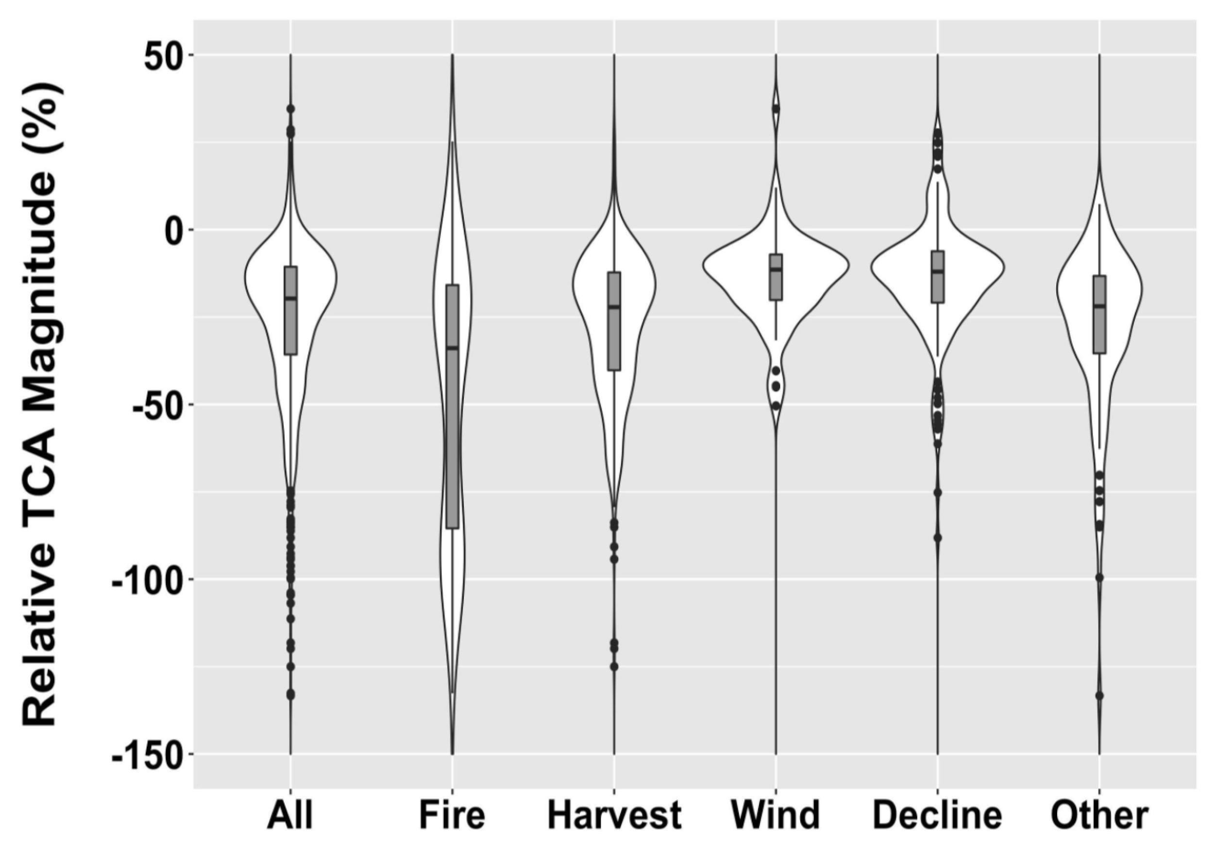
4.2. Disturbance Magnitude

Magnitude of forest disturbance is highly variable, with effects from concentrated tree mortality (or clearcutting) to minor adjustments in community structure and organization [3,39]. Although for a given, local disturbance, high-magnitude occurrences are very important, lower-magnitude disturbances are much more ubiquitous and can have a cumulative effect that is considerably greater [5,6,40]. This is particularly true in the era of climate change, where forest health is declining in many regions around the world [8,10]. Landsat data are at an appropriate spatial resolution for monitoring forest disturbance [7,13,41], and with major improvements in the quality and free availability of Landsat data over the past decade [14], a large number of advanced algorithms have begun to take advantage of dense Landsat time series to characterize and map forest disturbance (e.g., Table 1). However, it remains challenging for many of these algorithms to capture lower-magnitude disturbances, as demonstrated elsewhere (e.g., [22,29]) and in this study.

Our TimeSync reference data revealed a distribution of observed disturbances across the six study scenes that was skewed towards lower spectral change magnitudes (Figure 5), a result consistent with a more thorough, recent study across the conterminous US [6]. Further, we demonstrated here that the large majority of omitted disturbances in the maps derived from all the evaluated algorithms was associated with lower-magnitude disturbances (Figure 7, bottom). Based on this set of findings, it follows that there should be a relationship between the number of map sets that agreed with TimeSync disturbance observations and the magnitude of those observations, which was indeed the case (Figure 8).

By plotting omission rates as a function of magnitude, we can learn if there is commonality among the maps examined here, in terms of a magnitude threshold below which omission rates increase. Although omission rates were highly variable among the maps, their magnitude profiles were quite similar, with sharp declines from very low magnitudes (near zero) to about 50% relative TCA change magnitude, depending on the map set evaluated (Figure 9). This suggests quite notably that disturbances having relative TCA magnitudes below 50% are the more challenging ones for algorithms to capture and map. This is likely due to the fact that Landsat time series can be noisy because of imperfections in georeferencing, atmospheric correction, and calibration coefficients over time. For magnitudes below 50%, there may be a cost, in terms of commission error, to any given algorithm trying to exploit low-magnitude disturbance signals in Landsat time series data. This is somewhat obvious from the fact that most committed errors had very low spectral change magnitude distributions (Figure 7, top), not unlike the magnitude distributions of omitted errors.

Prior to the recent proliferation of algorithms designed to exploit subtle signals in Landsat time series data, the common forest disturbance mapping target was almost exclusively higher-magnitude (i.e., stand replacement) disturbances. Maps that represented only high-magnitude disturbances were compared against reference datasets that represented the same magnitude of disturbance. The definitions of disturbance were essentially the same in both the map and the reference data, only high-magnitude disturbances were targeted, and mapping errors were relatively low. In this new era of dense time series mapping, we have expanded our target population to include subtle disturbances, and to differing degrees the newer crop of algorithms digs deeper into the time series noise to extract disturbance signals. Relative to the inclusive reference dataset in our study, this had the effect of decreasing omission while increasing commission.

Because we used a very broad, inclusive definition of disturbance and evaluated all map products against this high standard, we have learned two important lessons. First, when an independent error assessment using such a highly inclusive reference dataset is conducted, we should expect higher mapping errors than those reported in earlier published results which are based on only subsets of the full range of disturbance magnitudes. Accordingly, mapping projects should clearly define disturbance in terms of either the spectral change magnitude or the percent tree cover affected. This will help map users better understand how to relate the error matrix to the map by taking into consideration the definition of disturbance employed.

Second, using an algorithm with current spatiotemporal densities of freely available remote sensing datasets to extract information about forest disturbances having spectral change magnitudes below a certain threshold (in terms of relative TCA magnitude, that is ~50%) will likely remain challenging and will be attended by increased levels of commission. However, there may be advantages to the use of multiple algorithms that reach into the realm of noise to extract change signals, if the different target populations and approaches are variable. For example, although the algorithms examined here had mixed success in detecting lower-magnitude disturbance, those successes were often non-overlapping, i.e., the majority of detected subtle changes were mapped by one or two algorithms for a given pixel. Despite this commission error (that might be considered the cost of sensitivity), these algorithms show that the Landsat archive does record somewhat subtle ecosystem changes. Thus, a new direction in change detection is the possibility of capitalizing on the collective sensitivities of innovative new algorithms by incorporating them into a learning ensemble (such as Random Forests [42]) using a training dataset (e.g., from TimeSync).

4.3. Why Are the Maps So Different?

Given the very different maps and summary disturbance results derived from the algorithms examined in this study, we now consider the factors that are likely responsible for such differences, including: (i) the basic algorithm logic; (ii) the density of Landsat observations; (iii) the magnitude threshold; (iv) the lack of training or calibration; and (v) the spectral dimensions utilized.

For the algorithms examined, there was a difference in the fundamental algorithm logic that likely had profound effects on the disturbance maps produced. Most algorithms were designed to discover anomalies in data trends over time. The classic example of this was the use of bi-temporal differencing, as represented by MIICA, where annual series of data were compared two sequential years at a time to determine whether a change had occurred in a given pixel over a given two-year period. Although not technically bi-temporal differencing, VCT, CCDC, and EWMACD (as implemented in this study) all specified change in terms of an anomalous departure from a trend in the spectral response over time. This logic for detecting forest change, almost by design, precluded the discovery of slowly trending spectral responses if there was never an observed departure from the overall trend in terms of a more sudden, dramatic disturbance representative of an anomaly. In contrast, ITRA was designed to seek gradual trends in the time series spectral response over approximately 10-year epochs. However, given that the characterization of a trend was based on the slope of a regression line over the epoch under consideration, it was highly likely that an observed trend was also influenced by anomalies. LandTrendr and VeRDET, by conducting an explicit temporal segmentation of the time series, were designed to discover both anomalies and trends in the data. In contrast to ITRA, these two algorithms let the data themselves dictate where to identify breaks in the time series, with anomalies lasting as little as one year and trends lasting as long as the full time-series length.

Density of Landsat observations was a critical difference in the algorithms’ approaches to disturbance characterization. LandTrendr, VeRDET, ITRA, MIICA, and VCT all used one Landsat observation per year, while CCDC and EWMACD used all available clear observations. To fill in for masked clouds and shadows, LandTrendr, VeRDET, and VCT all used image compositing rules with a logic that sought a consistent timing for observations among years, e.g., the peak of the growing season. ITRA and MIICA used synthetic, predicted data for 6 August of each year, based on the time series trend component of the CCDC algorithm. Using all available clear observations enabled CCDC and EWMACD to track phenology and seek anomalous departures from seasonal trends. This approach should be expected to discover changes in trends that occurred at any time of the year, as opposed to discovering only changes that were observable in the peak of the growing season. In theory, this should also have facilitated the detection of more subtle, anomalous changes, as many subtle changes are ephemeral.

Perhaps the most important difference among the algorithms examined here was the use of the spectral change magnitude thresholds. The application of a magnitude threshold to identify change (e.g., two standard deviations’ departure from a forest norming population for VCT) is a straightforward means for distinguishing between a change signal and the ubiquitous low-level spectral noise in a temporal series of Landsat data. Each algorithm used one or more thresholds to identify change, with the selected thresholds being associated with experience gained by algorithm developers during the application of their algorithms. One way to gauge the effect of the threshold on the results in this study was the comparative errors in omission and commission among maps. For example (Figure 2, top), evidence of higher thresholds for change can be found in the lower rates of disturbance mapped by VCT, CCDC, and MIICA. Lower thresholds for change were evident in the higher rates of disturbance associated with LandTrendr and EWMACD.

Calibrating an algorithm can be critical in the pursuit of accurate mapping results. Each algorithm used here, prior to this study, has had a different application domain, with some being limited to a few Landsat scenes from a given forested region of the US, whereas others have been much more widely applied. Regardless of the specific prior application domain, none of the algorithms were specifically calibrated for most of the six scenes used here. The high mapping errors observed during this study suggest strongly that to achieve low error rates, a given algorithm needs to be calibrated for the specific sets of forest type and disturbance regime conditions the algorithm will encounter. Moreover, given the levels of omission and commission observed, one might argue that beyond calibration, more explicit training of an algorithm, where the parameters of an algorithm are tuned to a training dataset, might be advantageous.

Another important consideration is the spectral band or index used by the algorithms. Several of the algorithms use only one spectral band or index (e.g., LandTrendr, EWMACD), whereas others (CCDC, MIICA) used multiple bands or indices. The expression of forest disturbance is band-dependent [15,16,17,18,19,20,21,22], and, regardless, no single band or index will likely optimize omission and commission, because forest disturbance has a multispectral expression.

5. Conclusions

This study tested seven modern change detection algorithms designed to use higher volumes of Landsat data than algorithms of the past. In this context, we compared their forest disturbance map products against a reference dataset that consisted of a highly inclusive set of disturbance observations. From this exercise, several conclusions emerged:

• Spectral change magnitudes associated with forest disturbance are highly variable, with a population likely to be skewed towards lower-magnitude occurrences. Such disturbances are challenging to map because they are often difficult to distinguish from spectral noise common in temporal trajectories of spectral signals.
• Landsat disturbance maps derived from automated algorithms are likely to be quite dissimilar. This is true both of the maps themselves and of aggregate rates of disturbance mapped over time.
• Maps from different algorithms are more likely to agree with each other about the location and timing of forest disturbance as the change magnitude becomes greater.
• Algorithms that target a broader set of disturbance magnitudes are likely to have more commission and less omission errors than algorithms that target mostly greater magnitude disturbances.
• A spectral change magnitude threshold (~50% relative TCA) was identified; for changes with a magnitude smaller than this threshold, the omission error increases. Algorithms that attempt to detect these lesser-magnitude disturbances are likely to exhibit greater levels of mapping commission.
• Users of forest disturbance maps now have choices among several maps, each derived from different algorithms. Given the strengths and weaknesses of each map with respect to the omission and commission errors and target disturbance populations, a user should be cautious and endeavor to understand how well these maps will suit their needs. It would be irresponsible to assume a given map is by default highly accurate and to not consider how errors might influence use in a variety of contexts.

References

1. Seidl, R.; Schelhaas, M.-J.; Rammer, W.; Verkerk, P.J. Increasing forest disturbance in Europe and their impacts on carbon storage. Nat. Clim. Chang. 2014, 4, 806–810. [Google Scholar] [CrossRef] [PubMed]
2. Turner, M.G. Disturbance and landscape dynamics in a changing world. Ecology 2010, 91, 2833–2849. [Google Scholar] [CrossRef] [PubMed]
3. McDowell, N.; Coops, N.C.; Beck, P.S.A.; Chambers, J.Q.; Gongodagamage, C.; Hicke, J.A.; Huang, C.; Kennedy, R.; Krofcheck, D.J.; Litvak, M.; et al. Global satellite monitoring of climate-induced vegetation disturbances. Trends Plant Sci. 2015, 20, 114–123. [Google Scholar] [CrossRef] [PubMed]
4. Schwantes, A.M.; Swenson, J.J.; Jackson, R.B. Quantifying drought-induced tree mortality in the open canopy woodlands of central Texas. Remote Sens. Environ. 2016, 181, 54–64. [Google Scholar] [CrossRef]
5. Brooks, E.B.; Wynne, R.H.; Thomas, V.A.; Blinn, C.E.; Coulston, J.W. On-the-fly massively multitemporal change detection using statistical quality control charts and Landsat data. IEEE Trans. Geosci. Remote Sens. 2014, 52, 3316–3332. [Google Scholar] [CrossRef]
6. Cohen, W.B.; Yang, Z.; Stehman, S.V.; Schroeder, T.A.; Bell, D.M.; Masek, J.G.; Huang, C.; Meigs, G.W. Forest disturbance in the conterminous US from 1985–2012: The emerging dominance of forest decline. For. Ecol. Manag. 2016, 360, 242–252. [Google Scholar] [CrossRef]
7. Cohen, W.B.; Goward, S.N. Landsat’s role in ecological applications of remote sensing. BioScience 2004, 54, 535–545. [Google Scholar] [CrossRef]
8. Allen, C.D.; Breshears, D.D.; McDowell, N.G. On underestimation of global vulnerability to tree mortality and forest die-off from hotter drought in the Anthropocene. Ecosphere 2015, 6, 1–55. [Google Scholar] [CrossRef]
9. Kennedy, R.E.; Yang, Z.; Cohen, W.B.; Pfaff, E.; Braaten, J.; Nelson, P. Spatial and temporal patterns of forest disturbance and regrowth within the area of the Northwest Forest Plan. Remote Sens. Environ. 2012, 122, 117–133. [Google Scholar] [CrossRef]
10. Mildrexler, D.; Yang, Z.; Cohen, W.B. A forest vulnerability index based on drought and high temperatures. Remote Sens. Environ. 2016, 173, 314–325. [Google Scholar] [CrossRef]
11. Sulle-Menashe, D.; Kennedy, R.E.; Yang, Z.; Braaten, J.; Krankina, O.; Friedl, M.A. Detecting forest disturbance in the Pacific Northwest from MODIS time series using temporal segmentation. Remote Sens. Environ. 2014, 151, 114–123. [Google Scholar] [CrossRef]
12. Kennedy, R.E.; Andréfouët, S.; Cohen, W.B.; Gómez, C.; Griffiths, P.; Hais, M.; Healey, S.P.; Helmer, E.; Hostert, P.; Lyons, M.B.; et al. Bringing an ecological view of change to Landsat- based remote sensing. Front. Ecol. Environ. 2014, 12, 339–346. [Google Scholar] [CrossRef]
13. Banskota, A.; Kayastha, N.; Falkowski, M.; Wulder, M.A.; Froese, R.E.; White, J.C. Forest monitoring using Landsat time-series data—A review. Can. J. Remote Sens. 2014, 40, 362–384. [Google Scholar] [CrossRef]
14. Wulder, M.A.; Masek, J.G.; Cohen, W.B.; Loveland, T.R.; Woodcock, C.E. Opening the archive: How free data has enabled the science and monitoring promise of Landsat. Remote Sens. Environ. 2012, 122, 2–10. [Google Scholar] [CrossRef]
15. Kennedy, R.E.; Yang, Z.; Cohen, W.B. Detecting trends in forest disturbance and recovery using yearly Landsat time series: 1. LandTrendr—Temporal segmentation algorithms. Remote Sens. Environ. 2010, 114, 2897–2910. [Google Scholar] [CrossRef]
16. Vogelmann, J.E.; Xian, G.; Homer, C.; Tolk, B. Monitoring gradual ecosystem change using Landsat time series analyses: Case studies in selected forest and rangeland ecosystems. Remote Sens. Environ. 2012, 122, 92–105. [Google Scholar] [CrossRef]
17. Huang, C.; Goward, S.N.; Masek, J.G.; Thomas, N. An automated approach for reconstructing recent forest disturbance history using dense Landsat time series stacks. Remote Sens. Environ. 2010, 114, 183–198. [Google Scholar] [CrossRef]
18. Jin, S.; Yang, L.; Danielson, P.; Homer, C.; Fry, J.; Xian, G. A comprehensive change detection method for updating the National Land Cover Database to circa 2011. Remote Sens. Environ. 2013, 132, 159–175. [Google Scholar] [CrossRef]
19. Zhu, Z.; Woodcock, C.E. Continuous change detection and classification of land cover using all available Landsat data. Remote Sens. Environ. 2014, 144, 152–171. [Google Scholar] [CrossRef]
20. Zhu, Z.; Woodcock, C.E.; Holden, C.; Yang, Z. Generating synthetic Landsat images based on all available Landsat data: Predicting Landsat surface reflectance at any given time. Remote Sens. Environ. 2015, 162, 67–83. [Google Scholar] [CrossRef]
21. Hughes, M.J. New Remote Sensing Methods for Detecting and Quantifying Forest Disturbance and Regeneration in the Eastern United States. Ph.D. Thesis, University of Tennessee, Knoxville, TN, USA, 2014. [Google Scholar]
22. Cohen, W.B.; Yang, Z.; Kennedy, R.E. Detecting trends in forest disturbance and recovery using yearly Landsat time series: 2. TimeSync—Tools for calibration and validation. Remote Sens. Environ. 2010, 114, 2911–2924. [Google Scholar] [CrossRef]
23. Schleeweis, K.; Goward, S.N.; Huang, C.; Masek, J.G.; Moisen, G.G.; Kennedy, R.E.; Thomas, N.E. Regional dynamics of forest canopy change and underlying causal processes in the contiguous U.S. J. Geophys. Res. Biogeosci. 2013, 118, 1035–1053. [Google Scholar] [CrossRef]
24. Reufenacht, B.; Finco, M.V.; Nelson, M.D.; Czaplewski, R.; Helmer, E.H.; Blackard, J.A.; Holden, G.R.; Lister, A.J.; Salajanu, D.; Weyerman, D.; Winterberger, K. Conterminous U.S. and Alaska forest type mapping using forest inventory and analysis data. Photogramm. Eng. Remote Sens. 2008, 74, 1379–1388. [Google Scholar] [CrossRef]
25. United State Geological Survey (USGS). Product Guide: Landsat 4–7 Climate Data Record (CDR) Surface Reflectance. 2016. Available online: http://landsat.usgs.gov/documents/cdr_sr_product_guide.pdf (accessed on 12 December 2016).
26. Masek, J.G.; Vermote, E.F.; Saleous, N.; Wolfe, R.; Hall, F.G.; Huemmrich, F.; Gao, F.; Kutler, J.; Lim, T.K. A Landsat Surface Reflectance Data Set for North America, 1990–2000. Geosci. Remote Sens. Lett. 2006, 3, 68–72. [Google Scholar] [CrossRef]
27. Zhu, Z.; Woodcock, C.E. Object-based cloud and cloud shadow detection in Landsat imagery. Remote Sens. Environ. 2012, 118, 83–94. [Google Scholar] [CrossRef]
28. Pflugmacher, D.; Cohen, W.B.; Kennedy, R.E. Comparison between Landsat-derived disturbance history and lidar to predict current forest structure. Remote Sens. Environ. 2012, 122, 146–165. [Google Scholar] [CrossRef]
29. Masek, J.G.; Goward, S.N.; Kennedy, R.E.; Cohen, W.B.; Moisen, G.G.; Schleeweis, K.; Huang, C. United States forest disturbance trends observed using Landsat time series. Ecosystems 2013, 16, 1087–1104. [Google Scholar] [CrossRef]
30. Olofsson, P.; Foody, G.M.; Herold, M.; Stehman, S.V.; Woodcock, C.E.; Wulder, M.A. Good practices for estimating area and assessing accuracy of land change. Remote Sens. Environ. 2014, 148, 42–57. [Google Scholar] [CrossRef]
31. Schroeder, T.A.; Healey, S.P.; Moisen, G.G.; Frescino, T.; Cohen, W.B.; Huang, C.; Kennedy, R.E.; Yang, Z. Improving estimates of forest disturbance by combining observa-tions from Landsat time series with US Forest Service Forest Inventory and Analysis data. Remote Sens. Environ. 2014, 154, 61–73. [Google Scholar] [CrossRef]
32. Powell, S.L.; Cohen, W.B.; Healey, S.P.; Kennedy, R.E.; Moisen, G.G.; Pierce, K.B.; Ohmann, J.L. Quantification of live aboveground forest biomass dynamics with Landsat time-series and field inventory data: A comparison of empirical modeling approaches. Remote Sens. Environ. 2010, 114, 1053–1068. [Google Scholar] [CrossRef]
33. Cochran, W.G. Sampling Techniques, 3rd ed.; John Wiley & Sons: New York, NY, USA, 1977; p. 428. [Google Scholar]
34. Avitabile, V.; Herold, M.; Henry, M.; Schmullius, C. Mapping biomass with remote sensing: A comparison of methods for the case study of Uganda. Carbon Balance Manag. 2011, 6, 1–14. [Google Scholar] [CrossRef] [PubMed]
35. Pflugmacher, D.; Krankina, O.N.; Cohen, W.B.; Friedl, M.; Sulla-Menashe, D.; Kennedy, R.; Nelson, P.; Loboda, T.; Kuemmerle, T.; Dyukarev, E.; et al. Comparison and assessment of coarse resolution land cover maps for Northern Eurasia. Remote Sens. Environ. 2011, 115, 3539–3553. [Google Scholar] [CrossRef]
36. Mitchard, E.T.A.; Saatchi, S.S.; Baccini, A.; Asner, G.P.; Goetz, S.J.; Harris, N.L.; Brown, S. Uncertainty in the spatial distribution of tropical forest biomass: A comparison of pan-tropical maps. Carbon Balance Manag. 2013, 8, 1–13. [Google Scholar] [CrossRef] [PubMed]
37. Cohen, W.B.; Spies, T.A.; Alig, R.J.; Oetter, D.R.; Maiersperger, T.K.; Fiorella, M. Characterizing 23 years (1972–1995) of stand replacement disturbance in western Oregon forests with Landsat imagery. Ecosystems 2002, 5, 122–137. [Google Scholar] [CrossRef]
38. Healey, S.P.; Cohen, W.B.; Spies, T.A.; Moeur, M.; Pflugmacher, D.; Whitley, M.G.; Lefsky, M.A. The Relative Impact of Harvest and Fire upon Landscape-Level Dynamics of Older Forests: Lessons from the Northwest Forest Plan. Ecosystems 2008, 11, 1106–1119. [Google Scholar] [CrossRef]
39. Dale, V.H.; Joyce, L.A.; McNulty, S.; Neilson, R.P.; Ayres, M.P.; Flannigan, M.D.; Hanson, P.J.; Irland, L.C.; Lugo, A.E.; Peterson, C.J.; et al. Climate change and forest disturbances. BioScience 2001, 51, 723–734. [Google Scholar] [CrossRef]
40. Espírito-Santo, F.D.B.; Gloor, M.; Keller, M.; Malhi, Y.; Saatchi, S.; Nelson, B.; Junior, R.C.O.; Pereira, C.; Lloyd, J.; Frolking, S.; et al. Size and frequency of natural forest disturbances and the Amazon forest carbon balance. Nat. Commun. 2014, 5, 3434. [Google Scholar] [PubMed]
41. Hansen, M.C.; Potapov, P.V.; Moore, R.; Hancher, M.; Turubanova, S.A.; Tyukavina, A.; Thau, D.; Stehman, S.V.; Goetz, S.J.; Loveland, T.R.; et al. High-resolution global maps of 21st-century forest cover change. Science 2013, 342, 850–853. [Google Scholar] [CrossRef] [PubMed]
42. Breiman, L. Random forests. Mach. Learn. 2001, 45, 5–32. [Google Scholar] [CrossRef]
Figure 1. Locations within the United States of the six study scenes (WRS-2 Path/Row). Forest type groups used by the US Forest Service, Forest Inventory and Analysis program are displayed for context (adapted from [24]).
Forests 08 00098 g001
Figure 2. (Top) Aggregate (across scene) disturbance rate trajectories for maps derived from each of the seven algorithms examined in this study, and for the TimeSync reference data (with 95% confidence interval envelope); (Bottom) Aggregate disturbance rate for TimeSync data (top), by causal agent class.
Forests 08 00098 g002
Figure 3. Example map sections for the year 2002 (middle and bottom rows), from each of the study scenes (top row), showing agreement among algorithm disturbance products. Boxes in top row show areas enlarged in middle and bottom rows.
Forests 08 00098 g003
Figure 4. Agreement among seven disturbance map sets over time, as a proportion of total disturbance mapped by all algorithms.
Forests 08 00098 g004
Figure 5. TimeSync reference data summary. Violin plots are based on disturbance occurrence counts across the six study scenes. Note that for subtle disturbances, TCA change values can be expressed in the unexpected direction (i.e., positive values).
Forests 08 00098 g005
Figure 6. Omission and commission rates for each of the seven map product sets. One-year offset allows for agreement between map disturbance and reference data to be off by one year.
Forests 08 00098 g006
Figure 7. Relative magnitude distributions for omission and commission occurrences from each of the seven map products.
Forests 08 00098 g007
Figure 8. Relative magnitude distributions for disturbance occurrences when no map (0) agreed with reference data, and for occurrences where between one and seven maps agreed.
Forests 08 00098 g008
Figure 9. Omission for the seven map product sets as a function of disturbance relative change magnitude.
Forests 08 00098 g009