Product and Residue Biomass Equations for Individual Trees in Rotation Age Pinus radiata Stands under Three Thinning Regimes in New South Wales, Australia

Abstract

Using data from 239 trees that were destructively sampled and completely weighed in the field, four systems of nonlinear additive equations were developed for the estimation of product and residue fresh and dry weight of individual trees in rotation age (28 to 42 years) Pinus radiata stands under three thinning regimes: unthinned (T0), one thinning (T1) and two thinnings (T2). To cater for all practical applications, the four systems of equations included diameter at breast height overbark (DBHOB) as the only independent variable or both DBHOB and total tree height as predictors either with or without the incorporation of dummy variables for stand types. For all systems, the property of additivity was guaranteed by placing constraints on the structural parameters of the system equations. The parameter estimates were obtained by the generalized methods of moments (GMM) following a comparison with weighted nonlinear seemingly unrelated regression (WNSUR). Based on the predicted values from the system that had DBHOB as the predictor and dummy variables for stand types, the percentage of total tree fresh weight accounted for by residues increased from 14.8% to 20.5%, from 15.6% to 22.2% and from 13.9% to 18.7% for trees in the T0, T1 and T2 stands, respectively, as DBHOB increased from 15 to 70 cm. The corresponding changes in the percentage of residue dry weight were from 15.1% to 16.1%, from 15.7% to 17.1% and from 14.9% to 15.8% for the three stand types. In addition, two systems of allocative equations were developed to allocate the predicted product and residue biomass to their respective subcomponents. The system of allocative equations for product biomass predicted that sawlogs with bark accounted for 83% to 85% of product fresh weight and 82% to 87% of product dry weight over the same range of DBHOB. The predicted allocation of total residue dry weight to stump changed little, between 12% and 13%, over the same diameter range, but it was slightly higher for trees with DBHOB between 30 and 45 cm. The predicted allocation of total residue biomass to branches increased from 18% to 65% in fresh weight and from 18% to 57% in dry weight and that to waste decreased from 71% to 27% in fresh weight and from 70% to 32% in dry weight as DBHOB increased from 15 to 70 cm. Among the five biomass components, prediction accuracy was the lowest for pulpwood and waste. The systems of additive and allocative biomass equations developed in this study provided the first example of how the two approaches could be used together for the estimation of total tree, major and sub-component biomass. They will provide forest management with an enhanced capacity to more accurately estimate product and residue biomass of rotation age trees and thus to include the production of biomass for renewable energy generation in their management systems for P. radiata plantations.

1. Introduction

After a plantation is harvested for wood products, there is usually a large amount of residue material left behind on the forest floor. The wood products are generally sawlogs and pulpwood; the residue material mainly consists of stumps, branches and tree tops, short off-cut and waste sections due to stem deformity, defects, damage and breakage. Over much of the latter half of the 20th Century, forest harvest residues represented a source of fuelwood for rural communities in many developing countries [1,2], while they were often windrowed, burned and mostly reduced to ashes to return to the soil as part of site preparation for the establishment of the next rotation in developed countries (e.g., [3,4,5]). With the increasing recognition of the role of bioenergy in climate change mitigation since the turn of the 21st Century (see [6,7,8]), forest harvest and timber processing residues have received a renewed focus as a major potential source of woody biomass that can be used to supplement or replace fossil fuels in order to reduce greenhouse gas emissions of energy production [9,10,11,12,13,14].

To realize this potential, the amount of product and residue biomass of individual trees needs to be estimated before it is scaled up for stands, compartments, the entire plantation or management area as part of growth and yield forecasting and harvest planning (e.g., [15,16]). Although there is a distinction between the measurements of mass and weight in strict terms of physics as noted by Parresol [17], dry weight is commonly used for biomass in scientific papers. Beyond the research community, however, fresh weight is also referred to as biomass in layman’s terms. Throughout the process of forest harvesting, residue collection, transportation and utilization, estimation of both fresh and dry weight of wood products, as well as harvest residues is necessary if research objectives and practical applications are both taken into consideration (see [18,19]). Estimates of product biomass can not only provide a baseline for the calculation of biomass of timber processing residues, but also facilitate the life-cycle-analysis of carbon stored in timber products over the long run (e.g., [11,20]). On the other hand, estimates of harvest residue biomass enable the calculation of its energy content and other material properties during subsequent residue processing as an energy source [21]. More importantly, as demonstrated by Smith et al. [22], Eisenbies et al. [15] and Jones et al. [23], these estimates provide the basis for the estimation of nutrient removals by collecting harvest residues for bioenergy and for the evaluation of the long-term implications of the removals on the nutrient budget, site productivity and the sustainability of plantations.

Pinus radiata D. Don, native to a Californian central coastal environment and to two Mexican islands off Baja California, is the most extensively planted exotic coniferous species in the Southern Hemisphere (see [24,25,26,27]). Because of its growth performance, responsiveness to management and cultivation and the usefulness of its wood for lumber, veneer and pulp, it has become the mainstay of the forest economy in Australia, Chile, New Zealand, Spain and South Africa, serving domestic markets and generating income from export [24,27,28,29,30]. It has also been planted in many other countries in both Hemispheres on eroded lands following deforestation and on degraded marginal agricultural lands to provide catchment protection, slope stabilisation, flood mitigation and erosion control and to generate environmental, ecological and social benefits in addition to timber harvests [24,27,31]. In southwest China in particular, it has emerged to be a suitable species for environmental plantings on steep and degraded mountain slopes for soil and water conservation along the upper reaches of the Yangtze River [32,33,34,35]. Now, the total planted area worldwide has well exceeded 4.2 million hectares and is still expanding [27]. In Australia alone, the current plantation estate is approximately 772,100 ha, and about one-third of this resource is in the State of New South Wales (NSW) [36].

With a rotation length between 18 and 40 years over different site classes among the major growing countries [27], the year-round harvesting of P. radiata plantations in any region of industrial scale production provides a continuous flow of product volume and residue biomass to be utilized for bioenergy generation. The use of end-of-rotation harvesting residues also reduces the amount of post-harvesting debris, eliminates the need to burn them on site and therefore minimises the cost of re-establishment. However, in comparison to the well-developed growth and yield models and prediction systems for product volumes of P. radiata over the last 40 years (see [37,38,39,40,41,42,43]), models for estimating harvest residue yield have so far remained in infancy. In a clear-felled 29-year-old stand with 360 trees/ha in New Zealand, logging residues amounted to about 15 percent of the stem dry weight [44]. In a 35-year-old stand in NSW, Australia, the dry weight of the crown section above the top log ranged from 7% to 33% with an average of 21% of the total aboveground tree dry weight [45]. In south-central Chile, the potential harvest residue biomass of individual trees amounted to an average of 29.2 ± 7.8% of their total aboveground biomass [46]. These results are dependent on the minimum merchantable small end diameter that is specified locally and on whether stem bark is taken as a part of harvest residue, as logs are often not debarked on the logging site, but in the sawmills. Therefore they offer a useful range of reference value for the estimation of product and residual biomass of individual trees, but cannot be generally applied to other rotation-age plantations with different site conditions, silvicultural regimes and merchantable log standards. Quantitatively, there is a lack of a systematic approach to the estimation of product and residual biomass and their respective components among these studies. A system of additive equations that takes into account the correlations among the biomass components and the logical constraints between the component and total tree biomass as demonstrated by Bi et al. [47] for P. radiata stands would be desirable. This study aimed to develop systems of equations for the estimation of product and residue biomass and their respective sub-component biomass in both fresh and dry weight for individual trees in rotation age P. radiata stands under three thinning regimes in NSW, Australia.

2. Material and Methods

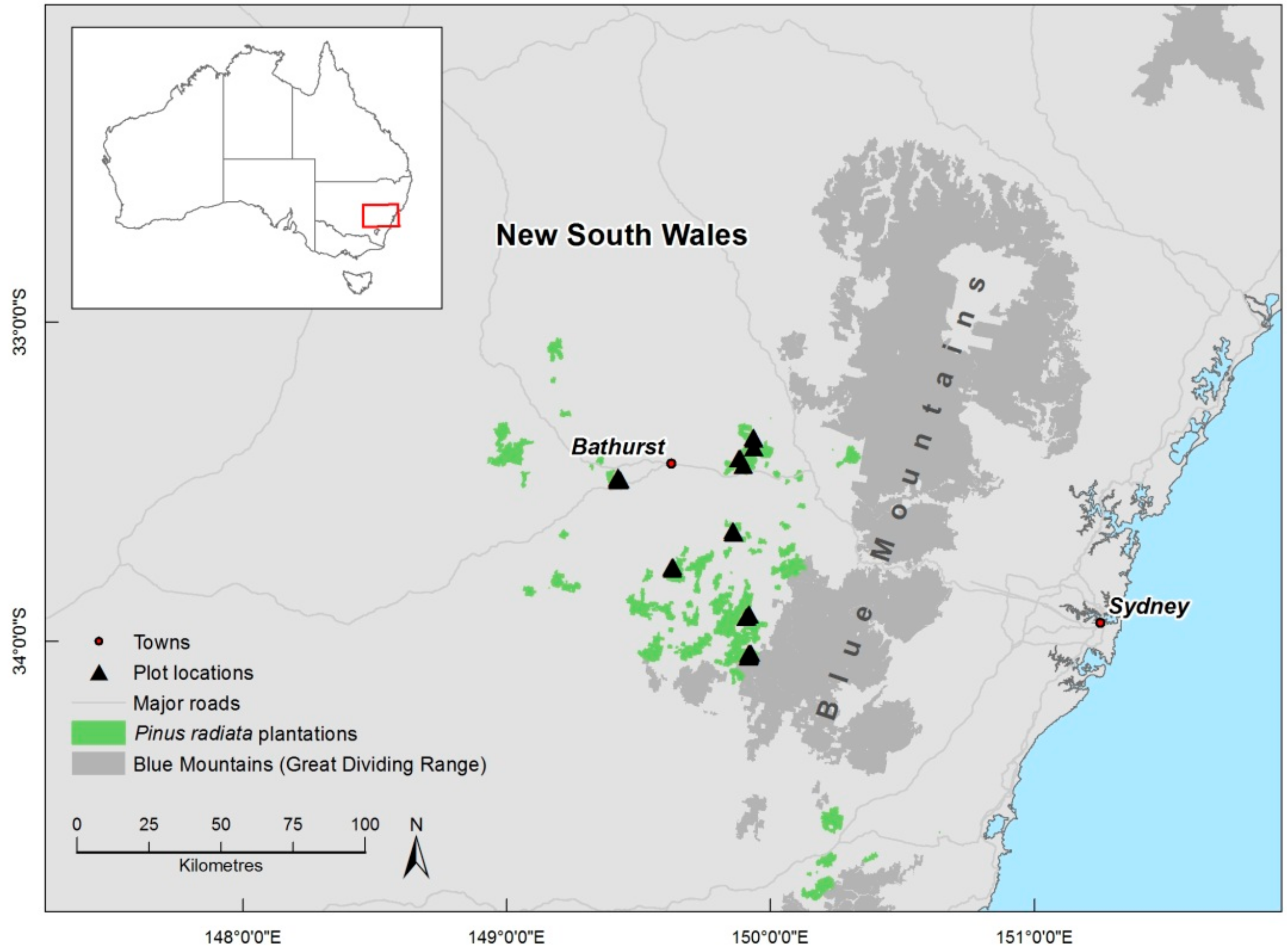
2.1. Study Area

The Bathurst management area of the Northern Softwood Region, Forestry Corporation of NSW (FCNSW), lies within latitudes 33°20′12” S to 34°0′48″ S and longitudes 149°22′57″ E to 149°53′57″ E on the central west slopes of NSW, Australia (Figure 1). Spanning an east-west distance of about 130 km and a north-south distance of about 190 km to the west of the Blue Mountain range, this management area encompasses 18 disjunct State Forest Plantations created by the state government from the 1910s all the way through the 1980s (see [48]). It has a declining altitude from about 1200 m around the mountain fringe in the east sloping down to approximately 750 m in the west. With the declining altitude from east to west, mean annual rainfall generally decreases from 1200 mm to 750 mm with an average about 900 mm, but the distribution of rainfall is relatively even throughout the year. The geology ranges from sandstone in the east, through a range of shales, siltstones, mudstones, greywacke with the odd granite intrusions and, towards the western edge of the management area, a range of acid lavas, dacite, trachyte and basalt areas [48]. Since the first commercial plantation of P. radiata was established in NSW a century ago, the ‘philosophy’ and practice of softwood plantation silviculture has evolved continuously [49]. The practice since the 1980s has been to set the initial planting stocking to 1000 to 1100 trees/ha. For more productive sites, either one or two thinnings are prescribed to reduce stocking down to 500 to 750 trees/ha at the age of first thinning around 15 years and down to 250 to 300 trees/ha at the age of second thinning around 25 years. For poorer sites, no thinning is specified before the final harvest generally at the age of 30 to 35 years. Currently the Bathurst management area has a total of 70,000 ha of P. radiata plantations established mostly after 1980 on ex-plantation, ex-pasture and ex-native forest sites (see [50]). These plantations are managed under the three thinning regimes: no thinning (T0), one thinning (T1) and two thinnings (T2). More than 2000 ha are harvested annually, supplying customers with 0.64 million m³ of sawlogs and 0.38 million m³ of pulpwood through long term wood supply agreements according to FCNSW’s 2016 forest management plan.

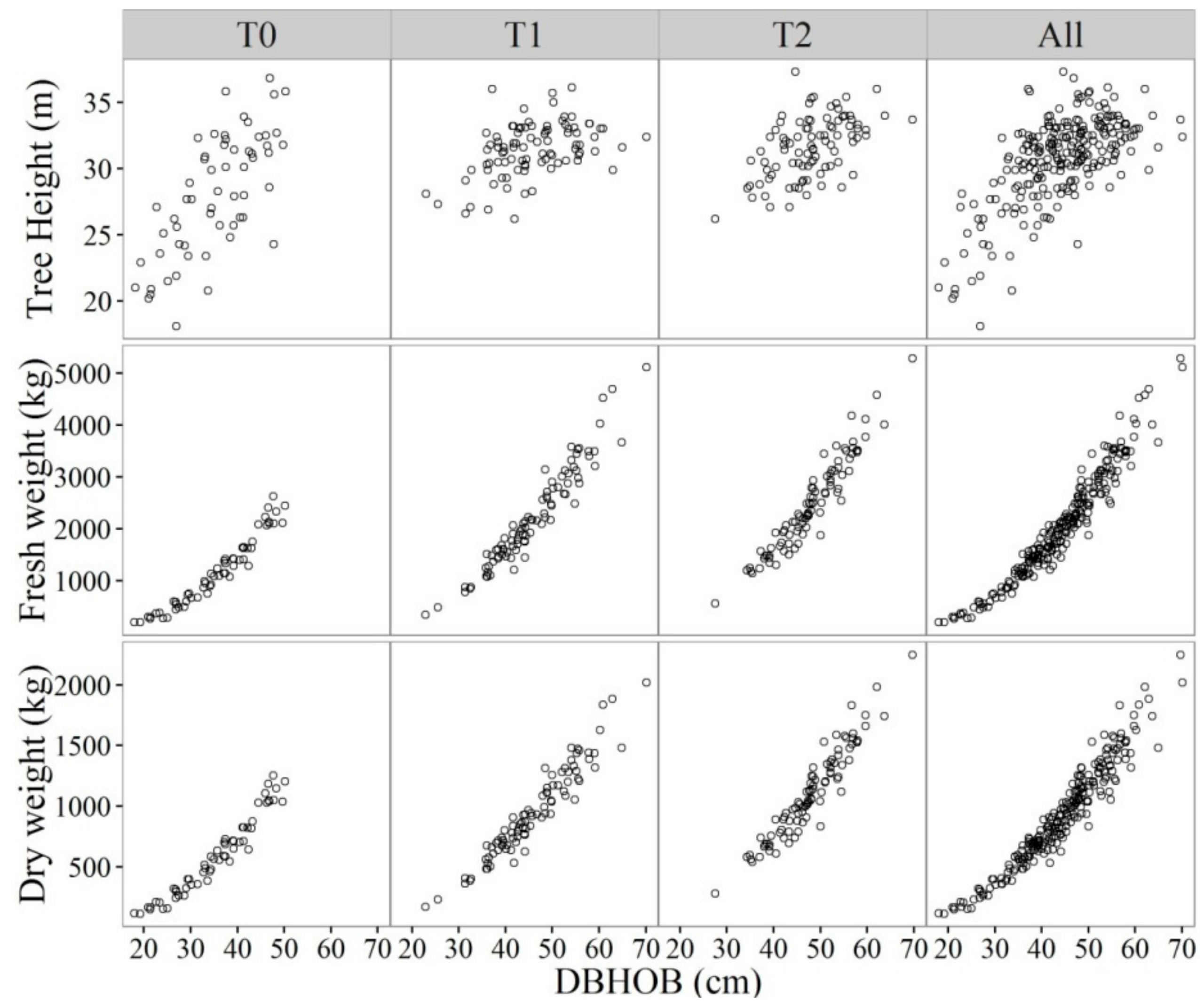
2.2. Plot Measurements and Selection of Sample Trees

Twelve sites with rotation-age stands over a range of site qualities were selected from five State Forests to represent the three thinning regimes for field sampling in 2011 (Figure 1). Their planting years varied from 1969 and 1983, corresponding to an age range between 28 and 42 years. Each site was a compartment with trees planted at the same time and managed under the same silvicultural regime. Five circular plots were established at each site. Plot centres were marked on the compartment map using randomly placed spatial locations in the office and located in the field using a hand-held GPS (Global Positioning System) device. Once a plot was located, a wooden peg was driven into the ground to mark the plot centre. Plot radius was generally 15 m for T0 stands, 20 m for T1 stands, and 25 m for T2 stands. The radius was varied so as to take in at least 30 to 40 trees in all plots across the three stand types. A total of 60 plots were established, including 30 in unthinned stands and 15 in each of the other two stand types (

Table 1. Stand attributes of plots in unthinned (T0), once-thinned (T1) and twice-thinned (T2) stands over the 12 sites. The range of each attribute was given together with its average in brackets. Dominant height was calculated as the average height of the 100 largest diameter trees/ha.

Thinning Type	Number of Plots	Age (Year)	Basal Area (m2/ha)	Dominant Height (m)	Stand Density (trees/ha)
T0	30	33–42 (39)	50.0–89.2 (64.4)	26.6–38.5 (31.5)	424–1188 (740)
T1	15	28–29 (28)	40.8–52.8 (46.8)	29.4–34.1 (31.8)	199–477 (325)
T2	15	28–33 (32)	30.5–46.6 (38.3)	29.3–37.3 (32.6)	163–366 (220)

). In each plot, diameter at breast height overbark (DBHOB) (at 1.3 m above ground level as defined in Australia) and the total tree height of all individual trees, either alive or dead, were measured to the nearest 0.1 cm and 0.1 m respectively using a diameter tape and a Vertex IV Ultrasonic Hypsometer made by Haglöf Sweden. At the same time, the trees were numbered sequentially with spray paint. Double leader trees that forked below breast height were measured in the same way as single leader trees.

Due to the lack of time and resources, destructive sampling was not carried out across all 12 sites, but only in 8 of them, including 2 T0, 3 T1 and 3 T2 sites. The eight sites were selected based on their accessibility by harvesting machinery, safety considerations and other topographical and operational constraints. For each selected site, trees on two out of the five plots were targeted for destructive sampling. Trees in each targeted plot were ranked in ascending order by their DBHOB first, then the cumulative basal area was calculated and then divided by the plot basal area to obtain the corresponding cumulative percentage of basal area, which was then divided into three even intervals, each representing one third of the plot basal area and a nominal dominance class of either suppressed or intermediate or dominant trees. Five trees were selected from each dominance class at random for destructive sampling, resulting in 15 targeted sample trees in each plot. For the 16 plots selected for destructive sampling across the 8 sites, a total of 240 sample trees were targeted, including 60 trees in 4 T0 plots, 90 in 6 T1 plots and the same number of trees in 6 T2 plots.

2.3. Destructive Sampling in the Field

The targeted sample trees were divided into two sampling groups: (1) fresh weight trees for obtaining the fresh weight only and (2) moisture content trees for taking additional subsamples to determine the dry to fresh ratio of biomass components. From the 15 targeted sample trees in each plot, three trees, one from each dominance class, were randomly selected as moisture content samples, except in one T2 plot where five trees were selected. Due to machinery breakdown, one of the 15 targeted trees was not sampled in a T0 plot. After several rounds of field sampling, a total of 239 trees, with DBHOB ranging from 18.0 to 70.1 cm and total tree height from 18.1 to 37.3 m, were destructively sampled from the 16 plots across the 8 sites. In addition to biomass sampling, three trees were selected from each plot for taper measurements, one randomly from each dominance class but avoiding trees with double leaders or deformities. Some of the 48 taper trees were among the trees selected for biomass sampling.

Except for the 48 taper trees, all sample trees were felled by a harvester equipped with a cutting head in a way to minimise breakage and damage to other trees during felling. The stump of each felled sample tree was marked with its corresponding tree number before stump height and diameter were measured. Stump height was measured from ground level on the high side of the stump to a point level with the top of the stump, while stump diameter was measured at or just under the stump height. Each felled tree was cut into logs, purposely without delimbing, by a chainsaw operator according to the commercial product specifications of the Northern Softwood Region where the minimum small end diameter overbark (SEDOB) was 15 cm for small sawlogs and 8 cm for pulpwood. Out of the 239 trees that were destructively sampled, there were 36 trees that produced sawlogs only but not any pulpwood. As often the case in harvesting operations, a small number of logs had to be cut just outside these specifications to minimise wastage and a number of short off-cut or waste sections had to be cut due to damage, deformity and breakage.

The logs with branches that were cut from each stem, including the waste sections if there were any, were picked up individually by a 25-ton excavator with a five finger hydraulic grab and moved to a pre-prepared log dump for delimbing, grading, marking and weighing. Special care was taken to ensure that branches were not lost through the hydraulic grab as the excavator moved from the felling spot through the standing trees to the log dump. However, a practically negligible amount of small twigs and needles might still be lost during this process. After landing at the log dump, branches were removed by chainsaw from individual logs and placed into corresponding piles. Then, the delimbed logs were graded and marked with spray paint to show their tree number, log number and log type before their lengths were measured using a measuring tape to the nearest 0.1 m. Regrettably the log end diameters were not measured just to save some time in the field as the project was under a very tight time constraint. These logs were picked up individually by the excavator and placed on a purpose-built biomass weighing trailer that was set up at the landing bay to obtain their fresh weight without debarking. The trailer was fitted with two weigh bars equipped with two load cells each and has a combined capacity of 5 tonnes and the smallest increment of 0.2 kg on a digital display (see [45]).

After weighing the logs and waste sections, the branches that were removed from the previously delimbed logs were weighed together with their needles. Large branches were picked up by the excavator and placed directly onto the two weigh bars located on both ends of the trailer. Small branches were manually placed on top of a plywood platform placed on the trailer to obtain their total fresh weight. Finally, the top part of the sample tree that was left after log cutting, customarily defined as the “crown” in this study, was sectioned into manageable lengths and sequentially coded before being brought by a forwarder to the landing bay where they were delimbed and weighed in separate bundles on the trailer. Some crown sections that consisted of secondary branches were weighed as a whole without delimbing.

From each of the 50 moisture content trees, three disks of approximately 5 cm in thickness with bark attached were cross-cut to represent the butt, mid and top section of the stem after the logs were weighed. The only exception was one tree in a T2 plot, from which five disks were cut. The butt disk was cut from the large end of the butt log and the top disk was cut from the small end of the top log. The mid-disk was not cut exactly at the mid-point of total tree length or total log length, but from the large end of either the second or the third or the fourth log depending on the number and length of logs cut from the stem. Cutting the disks in this way avoided creating an excessive amount of waste so that all the logs were still merchantable. A total of 152 disks were cut from the 50 moisture content trees. The disks from each tree were coded with their compartment, plot and tree numbers and the cutting positions before being placed into a tightly closed heavy duty plastic bag to avoid the loss of moisture and transported to the laboratory for further measurements, processing and analysis.

For each of the 48 taper trees, the total tree length was measured first by laying a straightened measuring tape from the felling point to the tip of the tree and then adding the stump height to the measurement. Diameter overbark (DOB) along the stem was then measured at pre-marked points starting at ground level or at a height as close to ground level as possible, then at a 0.5 m interval up to 2 m, and thereafter generally at a 2.0 m up to 12 m and from there onwards at about 4 m intervals until a small end diameter less or equal to 5 cm was recorded. When measurements could not be made at the marked measuring points due to swelling, defects, a branching point or whorl formation, the measuring points were moved up or down 0.1 m so that a normal part of the stem was measured.

2.4. Sample Processing and Oven Drying

Following each round of destructive sampling in the field, disk samples were brought back to the laboratory and stored in a cool room below 4 °C until they were processed shortly afterwards. For each disk, DOB and diameter underbark (DUB) were measured. Then the disks were weighed individually on a scale before and after debarking to obtain their fresh weight of wood and bark. Using a bandsaw, two V-shaped wedges were cut from the pith to the outer edge on the opposite sides of each debarked disk. The two wood wedges were weighed separately to obtain their fresh weights. At the same time, one sample of bark was taken and weighed. The two wood wedges and the bark sample were then placed in an aluminium tray labelled with their identification codes and oven-dried at 103 ± 2 °C until constant weight for the determination of moisture content in accordance with Australian/New Zealand Standard 1080.1 [51]. Drying at temperature higher than 80 °C may cause a loss of dry weight due to the decomposition of some organic compounds and volatilisation of some vegetative oils [52].

2.5. Calculating Stump Fresh Weight

As the stump of each sample tree was not extracted from the ground, it could not be weighed in the same way as the other parts of the tree. Therefore its fresh weight had to be calculated from the stump volume estimated using its stump diameter and height. Among the 239 sample trees, there were 13 trees in 5 plots across the three stand types that had missing stump diameter and also missing stump height values due to accidental damage during harvesting. Their diameters were estimated from the DBHOB of the corresponding sample trees using plot-specific linear least squares regression equations. Because there was little correlation between stump height and stump diameter, the missing values of stump height were estimated through multiple imputations by using the method of multivariate imputation by chained equations that was implemented in the R package, mice. A review of the statistical background and practical applications of mice in a wide range of fields could be found in Azur et al. [53] and van Buuren and Groothuis-Oudshoorn [54]. With the imputed missing values included, stump diameter varied from 20.6 to 84.9 cm with an average of 51.8 cm and stump height ranged from 5 to 44 cm with an average of 22.1 cm, except for one stump height of 81 cm in a T1 plot.

For the accurate estimation of stump volume over the butt swell, the trigonometric variable-form taper model of Bi [55] was fitted to the taper data from the 48 sample trees, but separately for T0, T1 and T2 stands. This model is stable in specification yet flexible in its ability of fitting data for species and tree sizes with different stem forms. Its predictive performance was well demonstrated for many native forest and plantation species in Australia [55,56]. For each of the 239 trees that were destructively sampled, an overbark taper curve was derived from its DBHOB and total tree height using the corresponding taper equation for its stand type. Then the predicted taper curve was calibrated using its stump height and diameter to generate a tree-specific overbark stem profile. Finally the stump volume was calculated through numerical integration of the tree-specific stem profile from ground level to stump height with an interval of 1 cm. At the same time, the volume of the butt log above the stump was also calculated by extending the numerical integration from the stump height over the log length. The ratio between the measured fresh weight and the calculated volume of the butt log was then used to convert the calculated stump volume to fresh weight for the sample tree. Following the calculation of stump fresh weight, the total aboveground fresh weight was calculated for each of the 239 sample trees (Figure 2).

2.6. Estimating Dry to Fresh Weight Ratios of Stemwood and Bark by Beta Regression

For every disk taken from each of the 50 moisture content trees, the dry to fresh weight ratio of wood (θ_w) was calculated as the average of that of the two wedges, while the dry to fresh weight ratio of bark (θ_b) was based on one sample. An exploratory analysis of θ_w and θ_b of all 152 disks showed a decreasing trend, albeit a considerable variation, as the sampling position moved up from the butt, through the mid, to the top sections of the stem. This trend and the associated variation suggested that relative height (RH), i.e., the height of the sampling position divided by the total tree height, was a key explanatory variable for both θ_w and θ_b within the tree. The exploratory analysis also indicated DBHOB and stand type might help to explain the variation in θ_w and θ_b between trees. As the logs cut from a stem varied in number and length, they also varied in the range of RH they represented. To convert log fresh weight to dry weight for the 239 sample trees, it would desirable to develop regression models that predict θ_w and θ_b from RH and other tree and stand variables. This approach would be far more accurate than simply using an average θ_w or θ_b for the butt, mid and top logs, but would require the RH of each sample disk be estimated. As the log end diameters were not measured, the RH of each disk was obtained through searching numerically the previously derived tree-specific stem profile for a value of DOB equal to the DOB of the disk. During the analysis, it was found that 6 disks had missing values of DOB. For these disks, DOB was estimated by using a simple linear relationship between DOB and DUB on log scales derived through the least squares regression. The log transformation bias was very small and practically negligible and so no correction was attempted.

As the values of θ_w and θ_b were fractional i.e., between 0 and 1, they were related to RH, DBHOB and the three stand types through beta regression using the R package, betareg (see [57]). Independently introduced by Paolino [58] and Ferrari and Cribari-Neto [59], but coined and popularized by the latter authors, beta regression has been widely adopted and proved to be a flexible approach for modelling continuous dependent variables on the standard unit interval (0,1) and it has also become an area of active research in applied statistics (see inter alia [60,61,62,63]). The beta regression model is based on the assumption that the response variable follows the beta distribution whose probability density function is characterized by two positive shape parameters, which, in combination, can generate very different shapes of distributions defined on the standard unit interval. Consequently beta regression renders itself a convenient and flexible approach for modelling rates and proportions. The two shape parameters were re-parameterized into a mean and a precision parameter for maximum likelihood estimation in betareg (see [57,59]). Consequently, the parameters of a beta regression model are estimated by the maximum likelihood method and the results have essentially the same interpretation as logistic regression [58,59].

Following a careful comparison of alternative variable transformations and equation forms, the following models were specified:

$$g\left({\theta }_w\right)=\left({\mathrm{w}}_1+{\mathrm{w}}_2{T}_2+{\mathrm{w}}_3{T}_0\right)+\left({\mathrm{w}}_4+{\mathrm{w}}_5{T}_2+{\mathrm{w}}_6{T}_0\right)\mathit{cos}\left(\frac{\pi }{2}RH\right) +{\mathrm{w}}_7\mathit{ln}D$$

(1)

and:

$$g\left({\theta }_b\right)=\left({\mathrm{b}}_1+{\mathrm{b}}_2{T}_2+{\mathrm{b}}_3{T}_0\right)+{\mathrm{b}}_4 RH+{\mathrm{b}}_5 lnD$$

(2)

where $g(·)$ is the logit link function i.e., $g\left(\mu \right)=log\left(\mu /\left(1-\mu \right)\right)$, ${\mathrm{w}}_1-{\mathrm{w}}_7$ and ${\mathrm{b}}_1-{\mathrm{b}}_5$ are coefficients, ln represents the natural logarithm, D stands for DBHOB in cm, cos is the cosine function, and RH, the relative height of the sample disk, is between 0 and 1. $T_2$ and $T_0$ in the equations are indicator or dummy variables representing twice thinned and unthinned stands respectively, they equal to one for the stand type they represent and zero otherwise. As described in Ferrari and Cribari-Neto [59], the pseudo-${\mathrm{R}}^2$, defined as the square of the correlation coefficient between observed and predicted logit transformed dependent variables, was computed by the betareg package as a measure of the variation explained by the regression. Once the equations were estimated, the predicted values of ${\theta }_w$ and ${\theta }_b$ were obtained by taking the inverse of the logit.

2.7. Estimating the Percentage of Bark Fresh Weight of Stem Sections

Although ${\theta }_w$ and ${\theta }_b$ were estimated through Equations (1) and (2) for a tree stem, they could not be used directly to convert the fresh weight of any stem section to dry weight because all stem sections and stumps were weighed or calculated in their entirety without debarking. Therefore the total fresh weight of a stem section had to be partitioned into wood and bark first before the estimated values of ${\theta }_w$ and ${\theta }_b$ could be applied for dry weight conversion. To do so, it would be ideal to use the fraction of bark in the fresh weight of each of the 152 sample disks as described in the preceding section. However, the fresh weight of disks before and after debarking was only available for 21 disks from 9 trees due to an unexpected loss of some weighing records. Using the data from these disks, the fraction of bark in the total fresh weight of a disk was related to RH and DBHOB as follows:

$$g\left({\theta }_{fb}\right)=\mathrm{a}+\mathrm{b}RH+\mathrm{c}R{H}^2+\mathrm{d}\mathit{ln}D$$

(3)

where ${\theta }_{fb}$ represents the fraction of bark fresh weight, a, b, c and d were coefficients to be estimated by beta regression. The estimated values of bark fractions were obtained by taking the inverse of the logit and then were converted to percentages by a multiplication of 100.

2.8. Converting Fresh Weight to Dry Weight

The fresh weight of a log was converted to dry weight through numerical integration of a large number of thinly sliced cross sections in the computer as follows:

$$D{W}_L={\displaystyle \sum }_{i=1}^n\left(\frac{V_i}{V_L}F{W}_L{\theta }_{fb}\left(R{H}_i\right){\theta }_b\left(R{H}_i\right)+\frac{V_i}{V_L}F{W}_L\left(1-{\theta }_{fb}\left(R{H}_i\right)\right){\theta }_w\left(R{H}_i\right)\right)$$

(4)

where $D{W}_L$ and $F{W}_L$ are the dry and fresh weight of a log or stem section of a sample tree in kg, $i$ indicates the $i$th step with a specified step size of 0.01 m in the numerical integration, $n$ equals the log length in m divided by the step size, $V_i$ is the corresponding overbark cross sectional volume in ${\mathrm{m}}^3$ calculated using the previously derived stem profile of the sample tree, $V_L={{\displaystyle \sum }}_{i=1}^n{V}_i$ is the overbark volume of the log in ${\mathrm{m}}^3$, $R{H}_i$ is the relative height of the upper surface of the $i$th cross section, ${\theta }_{fb}\left(R{H}_i\right)$ is the estimated fraction of bark at $R{H}_i$ from Equation (3), ${\theta }_b\left(R{H}_i\right)$ and ${\theta }_w\left(R{H}_i\right)$ are the corresponding dry to fresh weight ratios of bark and wood estimated from Equations (2) and (1). The fresh weight of stumps and waste sections were converted to dry weight in the same way.

For all branches of the sample tree, the conversion was not through numerical integration but was made directly as follows:

$$D{W}_B=F{W}_B{\theta }_{fb}\left(0.95\right){\theta }_b\left(0.95\right)+F{W}_B\left(1-{\theta }_{fb}\left(0.95\right)\right){\theta }_w\left(0.95\right)$$

(5)

where $D{W}_B$ and $F{W}_B$ are the dry and fresh weight of all branches of the sample tree in kg, ${\theta }_{fb}\left(0.95\right)$, ${\theta }_b\left(0.95\right)$ and ${\theta }_w\left(0.95\right)$ are the estimated values of ${\theta }_{fb}$, ${\theta }_b$ and ${\theta }_w$ from Equations (3), (2) and (1) at RH = 0.95. This particular value of relative height was selected by comparing the observed range of branch diameter with the distribution of estimated stem DOB at RH = 0.95 for all 239 samples trees using the overbark taper equations for the stand types. The branch diameter of sample trees varied from less than 2 cm to greater than 8 cm and the estimated stem DOB at RH = 0.95 varied from 1.7 cm to 10.8 cm but was mostly (i.e., greater than 95% of the cases) less than 8 cm. The two size ranges had an almost complete overlap.

2.9. Systems of Additive and Allocative Biomass Equations

The total aboveground biomass of a tree in our study consisted of two major components: product and residue biomass. Each major component could be broken down into two or three subcomponents: sawlogs and pulpwood for product biomass, and stumps, branches, short off-cut and waste sections including stem tops for residue biomass. Considering the hierarchical nature of the biomass data and the practical applications of the biomass equations in forest management, a two-step approach was adopted in the development of biomass equations for the major and sub-components. In the first step, systems of additive equations were developed to predict the total biomass of the tree and the biomass of its two major components. In the second step, a system of allocative biomass equations was developed for each major component to predict the biomass of its sub-components. The two systems of equations, when used together, would enable the prediction of the total and all major and sub-component biomass of individual trees.

2.9.1. Additive Biomass Equations

To cater for all practical applications in forest management, four systems of nonlinear additive equations were specified following the approaches of Parresol [64], Bi et al. [65] and Bi et al. [66]. The first system of additive equations had the simplest model form:

$$\begin{gathered} Y_{prod}={\mathsf{\beta }}_{10}{D}^{{\mathsf{\beta }}_{11}}+{\epsilon }_1 \\ {Y}_{res}={\mathsf{\beta }}_{20}{D}^{{\mathsf{\beta }}_{21}}+{\epsilon }_2 \\ {Y}_{total}={\mathsf{\beta }}_{10}{D}^{{\mathsf{\beta }}_{11}}+{\mathsf{\beta }}_{20}{D}^{{\mathsf{\beta }}_{21}}+{\epsilon }_3 \end{gathered}$$

(6)

where $Y_{prod}$, $Y_{res}$ and $Y_{total}$ represent product, residue and total tree biomass, either in fresh or dry weight, in kg respectively, D represents DBHOB in cm, ${\mathsf{\beta }}_{\mathrm{ij}}$ are coefficients, and ${\epsilon }_1$ to ${\epsilon }_3$ are the corresponding error terms. The error terms are inherently correlated and can be expressed as a vector

$$\epsilon ={\left[{\epsilon }_1,{\epsilon }_2,{\epsilon }_3\right]}^{\prime }$$

(7)

with the expectation $E(\epsilon$) = 0 and a variance and covariance matrix $E\left(\epsilon {\epsilon }^{\prime }\right)=\Sigma$. Each coefficient in the model is shared between two equations in order to ensure additivity of biomass estimates. Based on this model specification and some further exploratory analysis, the second system of equations incorporated total tree height as an additional predictor as follows:

$$\begin{gathered} Y_{prod}={\mathsf{\beta }}_{10}{D}^{{\mathsf{\beta }}_{11}}{H}^{{\mathsf{\beta }}_{12}}+{\epsilon }_1 \\ {Y}_{res}={\mathsf{\beta }}_{20}{D}^{{\mathsf{\beta }}_{21}}+{\epsilon }_2 \\ {Y}_{total}={\mathsf{\beta }}_{10}{D}^{{\mathsf{\beta }}_{11}}{H}^{{\mathsf{\beta }}_{12}}+{\mathsf{\beta }}_{20}{D}^{{\mathsf{\beta }}_{21}}+{\epsilon }_3 \end{gathered}$$

(8)

where H represents total tree height in m, ${\mathsf{\beta }}_{\mathrm{ij}}$ are coefficients. H was not incorporated as a predictor for $Y_{res}$ as it was not a statistically significant predictor for the residue component. The third and fourth systems of equations incorporated stand types as dummy variables in model (6) and (8):

$$\begin{gathered} Y_{prod}={\mathsf{\beta }}_{10}{D}^{\left({\mathsf{\beta }}_{11}+{\mathsf{\beta }}_{\mathrm{d}11}{T}_2+{\mathsf{\beta }}_{\mathrm{d}12}{T}_0\right)}+{\epsilon }_1 \\ {Y}_{res}={\mathsf{\beta }}_{20}{D}^{\left({\mathsf{\beta }}_{21}+{\mathsf{\beta }}_{\mathrm{d}21}{T}_2+{\mathsf{\beta }}_{\mathrm{d}22}{T}_0\right)}+{\epsilon }_2 \\ {Y}_{total}={\mathsf{\beta }}_{10}{D}^{\left({\mathsf{\beta }}_{11}+{\mathsf{\beta }}_{\mathrm{d}11}{T}_2+{\mathsf{\beta }}_{\mathrm{d}12}{T}_0\right)}+{\mathsf{\beta }}_{20}{D}^{\left({\mathsf{\beta }}_{21}+{\mathsf{\beta }}_{\mathrm{d}21}{T}_2+{\mathsf{\beta }}_{\mathrm{d}22}{T}_0\right)}+{\epsilon }_3 \end{gathered}$$

(9)

and:

$$\begin{gathered} Y_{prod}={\mathsf{\beta }}_{10}{D}^{\left({\mathsf{\beta }}_{11}+{\mathsf{\beta }}_{\mathrm{d}11}{T}_2+{\mathsf{\beta }}_{\mathrm{d}12}{T}_0\right)}{H}^{{\mathsf{\beta }}_{12}}+{\epsilon }_1 \\ {Y}_{res}={\mathsf{\beta }}_{20}{D}^{\left({\mathsf{\beta }}_{21}+{\mathsf{\beta }}_{\mathrm{d}21}{T}_2+{\mathsf{\beta }}_{\mathrm{d}22}{T}_0\right)}+{\epsilon }_2 \\ {Y}_{total}={\mathsf{\beta }}_{10}{D}^{\left({\mathsf{\beta }}_{11}+{\mathsf{\beta }}_{\mathrm{d}11}{T}_2+{\mathsf{\beta }}_{\mathrm{d}12}{T}_0\right)}{H}^{{\mathsf{\beta }}_{12}}+{\mathsf{\beta }}_{20}{D}^{\left({\mathsf{\beta }}_{21}+{\mathsf{\beta }}_{\mathrm{d}21}{T}_2+{\mathsf{\beta }}_{\mathrm{d}22}{T}_0\right)}+{\epsilon }_3 \end{gathered}$$

(10)

where $T_2$ and $T_0$ are indicator or dummy variables as previously defined in Equation (2). Similar approaches of incorporating dummy variables in a single or a system of biomass equations can be found in Bi et al. [65], Zeng et al. [67] and Fu et al. [68,69]. For residue dry weight in Equations (9) and (10), the dummy variables for stand types were later removed from the model specification because they proved to be statistically non-significant following subsequent model fittings as described below.

Because of the existence of heteroscedasticity in the error terms, the four systems of nonlinear additive biomass equations were fitted to the data using the GMM in the PROC MODEL procedure of SAS/ETS. This method produces efficient parameter estimates under heteroscedastic conditions without any specification of the nature of the heteroscedasticity [70], and so has been used for parameter estimation of system of additive biomass equations (e.g., [47,65,66]). In addition, the four systems of equations were also fitted to the data using WNSUR as demonstrated by Parresol [64]. Comparisons of the two methods of parameter estimation in terms of their mean squared errors for the system equations indicated that GMM was slightly better than WNSUR. Therefore, the parameter estimates obtained using GMM were reported in the paper.

2.9.2. Allocative Biomass Equations

In the four systems of additive equations described above, the total aboveground biomass of a tree was specified to be the sum of the biomass of its two major components i.e., product and residue. This type of model specification represents a bottom-up approach and has been well known and widely applied in the western literature. Once the biomass of the major components was estimated in the first step, a top-down approach was needed in the second step to allocate the estimated biomass of each major component to its subcomponents. Such a top-down approach was developed within the framework of error-in-variable models by Tang et al. [71,72]. Although being predominantly used in China for developing “compatible” biomass equations, it has had only a limited exposure outside China (see [73]). Taking this top-down approach, the following system of equations was specified to allocate the predicted total product biomass from the additive equations in Step 1 to sawlog and pulpwood biomass:

$$\begin{gathered} Y_{saw}=\frac{{\mathrm{a}}_{11}{D}^{{\mathrm{b}}_{11}}}{{\mathrm{a}}_{11}{D}^{{\mathrm{b}}_{11}}+{\mathrm{a}}_{12}{D}^{{\mathrm{b}}_{12}}}{\widehat{Y}}_{prod}+{\epsilon }_{11} \\ {Y}_{pulp}=\frac{{\mathrm{a}}_{12}{D}^{{\mathrm{b}}_{12}}}{{\mathrm{a}}_{11}{D}^{{\mathrm{b}}_{11}}+{\mathrm{a}}_{12}{D}^{{\mathrm{b}}_{12}}}{\widehat{Y}}_{prod}+{\epsilon }_{12} \end{gathered}$$

(11)

where $Y_{saw}$ and $Y_{pulp}$ stands for sawlog and pulpwood biomass in either fresh or dry weight in kg, ${\widehat{Y}}_{prod}$ represents the corresponding predicted total product biomass in kg from any of the systems of additive equations, ${\mathrm{a}}_{\mathrm{ij}}$ and ${\mathrm{b}}_{\mathrm{ij}}$ are coefficients, ${\epsilon }_{11}$ and ${\epsilon }_{12}$ are the error terms. The numerators of the first and the second system equation relate $Y_{saw}$ and $Y_{pulp}$ to D through a simple power function, while the denominator of both equations is the sum of the two numerators. Once the two equations are estimated as one system and summed up, it becomes self-evident that ${\widehat{Y}}_{saw}+{\widehat{Y}}_{pulp}={\widehat{Y}}_{prod}$, i.e., the total product biomass is logically broken down and allocated to its sawlog and pulpwood subcomponents. As the parameters each appeared three times in the two system equations, they were re-parameterized as shown below for parameter estimation:

$$\begin{gathered} Y_{saw}=\frac{1}{1+{\mathrm{r}}_{11}{D}^{{\mathrm{r}}_{12}}}{\widehat{Y}}_{prod}+{\epsilon }_{11} \\ {Y}_{pulp}=\frac{{\mathrm{r}}_{11}{D}^{{\mathrm{r}}_{12}}}{1+{\mathrm{r}}_{11}{D}^{{\mathrm{r}}_{12}}}{\widehat{Y}}_{prod}+{\epsilon }_{12} \end{gathered}$$

(12)

where ${\mathrm{r}}_{11}={\mathrm{a}}_{12}/{\mathrm{a}}_{11}$, and ${\mathrm{r}}_{12}={\mathrm{b}}_{12}-{\mathrm{b}}_{11}$. In the same way, a system of allocative biomass equations was specified to allocate the estimated total residue biomass in Step 1 to the three subcomponents:

$$\begin{gathered} Y_{stump}=\frac{1}{1+{\mathrm{r}}_{21}{D}^{{\mathrm{r}}_{22}}+{\mathrm{r}}_{23}{D}^{{\mathrm{r}}_{24}}}{\widehat{Y}}_{res}+{\epsilon }_{21} \\ {Y}_{branch}=\frac{{\mathrm{r}}_{21}{D}^{{\mathrm{r}}_{22}}}{1+{\mathrm{r}}_{21}{D}^{{\mathrm{r}}_{22}}+{\mathrm{r}}_{23}{D}^{{\mathrm{r}}_{24}}}{\widehat{Y}}_{res}+{\epsilon }_{22} \\ {Y}_{waste}=\frac{{\mathrm{r}}_{23}{D}^{{\mathrm{r}}_{24}}}{1+{\mathrm{r}}_{21}{D}^{{\mathrm{r}}_{22}}+{\mathrm{r}}_{23}{D}^{{\mathrm{r}}_{24}}}{\widehat{Y}}_{res}+{\epsilon }_{23} \end{gathered}$$

(13)

where $Y_{stump}$, $Y_{branch}$ and $Y_{waste}$ represent for stump, branch, and waste biomass in either fresh or dry weight in kg, ${\widehat{Y}}_{res}$ represents the corresponding predicted total residue biomass in kg from any of the systems of additive equations, ${\mathrm{r}}_{21}$, ${\mathrm{r}}_{22}$, ${\mathrm{r}}_{23}$ and ${\mathrm{r}}_{24}$ are coefficients, ${\epsilon }_{21}$, ${\epsilon }_{22}$ and ${\epsilon }_{23}$ are the error terms.

As there were 36 trees that produced sawlogs only but not any pulpwood during destructive sampling, the data for estimating Equation (12) came from the remaining 203 trees that produced both products. The data for estimating Equation (13) came from all 239 sample trees. The two allocative systems were initially fitted to the data as nonlinear error-in-variable models with derived weight functions to overcome heteroscedasticity using ForStat 2.2, the statistical software developed by the Chinese Academy of Forestry in Beijing and documented in detail by Tang et al. [74]. The theoretical background and technical details of the statistical model specification and parameter estimation can be found in Tang et al. [71,72,74] and Dong et al. [73]. When the number of equations is equal to the number of variables with errors in the system, the equations can be regarded as a system of simultaneous equations [74]. In such cases, the system of allocative equations can also be estimated by WNSUR and GMM using the PROC MODEL Procedure of SAS. As demonstrated by Dong et al. [73] with an allocative system of biomass equations, ForStat and the SAS procedure produced almost identical parameter estimates and jackknifing validation statistics. Therefore, Models (12) and (13) were also estimated by WNSUR and GMM using the PROC MODEL procedure. Comparisons of the two methods of parameter estimation in terms of their mean squared errors for the system equations indicated that GMM was slightly better than WNSUR. Therefore, the parameter estimates obtained using GMM were reported in the paper.

2.9.3. Residual Variance and Approximate Confidence Band of Residuals

To quantify the spread of observed values of biomass about their predicted values, residual variance and approximate confidence band containing about 90% of the observed data about the mean curve of predicted biomass were derived for all additive biomass equations using the method of Bi et al. [66]. The residual variance, $Var\left(\epsilon \right)$, was assumed to be a power function of the estimated mean, $\widehat{Y}$, as follows:

$$Var\left(\epsilon \right)\approx {\sigma }^2{\widehat{Y}}^{\mathrm{b}}$$

(14)

where ${\sigma }^2$ is a scale factor and b is a coefficient. The theoretical background of this method is described in detail in the context of estimated generalized least squares in econometric texts [70,75]. Following previous applications in modelling residual heteroscedasticity (e.g., [64,65,66]), the squares of residuals (${\epsilon }^2$) were used as representatives of their variances:

$${\epsilon }^2={\sigma }^2{\widehat{Y}}^{\mathrm{b}}$$

(15)

As in Bi et al. [66], Equation (15) was linearized first by taking logarithmic transformation of both sides and then estimated by using the GENMOD procedure of SAS where an exchangeable correlation matrix was specified as the working correlation structure to take into account the inherent correlation of sample trees from the same plot. For the systems of equations that incorporated the three thinning treatments, two dummy variables were used in the linearized equation to represent the three stand types. As the residual variance function was estimated using log transformed data, it had an inherent bias when back transformed from logarithm. To reduce such bias, Snowdon’s [76] bias correction factor (${\theta }_s$) was calculated for the residual variance function of each system equation. The square root of the variance function with bias correction was used to weigh the residuals. The 5th and 95th percentiles from the distribution of weighted residuals were taken as the approximate lower and upper confidence limits of residual error at the 90% level. For any predicted value of a biomass, $\widehat{Y}$, the approximate 90% confidence band of the observed data were delineated by:

$$\left(\widehat{Y}+p_5\sqrt{{\theta }_S{\sigma }^2{\widehat{Y}}^{\mathrm{b}}}, \widehat{Y}+p_{95}\sqrt{{\theta }_S{\sigma }^2{\widehat{Y}}^{\mathrm{b}}}\right)$$

(16)

where $p_5$ and $p_{95}$ are the 5th and 95th percentiles of the distribution of weighted residuals. Confidence intervals thus obtained were not necessarily symmetric about zero since the distribution of weighted residuals may be skewed.

2.9.4. Evaluating Prediction Accuracy

To evaluate how accurately the systems of biomass equations would perform in practice with an independent dataset, a leave-one-plot-out cross-validation procedure was carried out for both fresh and dry weight of all biomass components. In doing so, all previously specified systems of additive and allocative equations were fitted 16 times. Each time, sample trees from one of the 16 plots were left out from the fitting process and the predicted values of total tree biomass, all major and sub-component biomass were obtained from the systems of equations estimated using the remaining data from the other 15 plots. Using the observed and predicted values of all 239 sample trees following the repeated fitting, six benchmarking statistics, including the mean error of prediction (MEP), the mean percentage error of prediction (MPEP), the mean absolute error of prediction (MAEP), the mean percentage absolute error of prediction (MPAEP), the mean squared error of prediction (MSEP) and the prediction coefficient of determination (${\mathrm{R}}_{\mathrm{p}}^2$), were calculated as follows:

$$\mathrm{MEP} ={\displaystyle \sum }_{i=1}^n(y_i-{\widehat{y}}_i)/n$$

(17)

$$\mathrm{MPEP}=100\times {\displaystyle \sum }_{i=1}^n\left(\frac{y_i-{\widehat{y}}_i}{{\widehat{y}}_i}\right)/n$$

(18)

$$\mathrm{MAEP} ={\displaystyle \sum }_{i=1}^n|y_i-{\widehat{y}}_i|/n$$

(19)

$$\mathrm{MPAEP} =100\times {\displaystyle \sum }_{i=1}^n\left|\frac{y_i-{\widehat{y}}_i}{{\widehat{y}}_i}\right|/n$$

(20)

$$\mathrm{MSEP} ={\displaystyle \sum }_{i=1}^n\left(y_i-{\widehat{y}}_i{)}^2\right)/n$$

(21)

$${\mathrm{R}}_p^2 = 1 -\left({\displaystyle \sum }_{i=1}^n{\left(y_i-{\widehat{y}}_i\right)}^2/{\displaystyle \sum }_{i=1}^n{\left(y_i-\overline{y}\right)}^2\right)$$

(22)

where $y_i$ represents the observed value of total or component biomass of the i-th tree in kg, ${\widehat{y}}_i$ stands for the predicted value of $y_i$, $\overline{y} = {{\displaystyle \sum }}_{i=1}^n{y}_i/n$ is the mean of the observed values, and n equals 239, the total number of sample trees. As reviewed by Huang et al. [77], these benchmarking statistics have been commonly used in evaluating the predictive performance of forest models as they assess the size, direction and dispersion of the prediction error.

3. Results

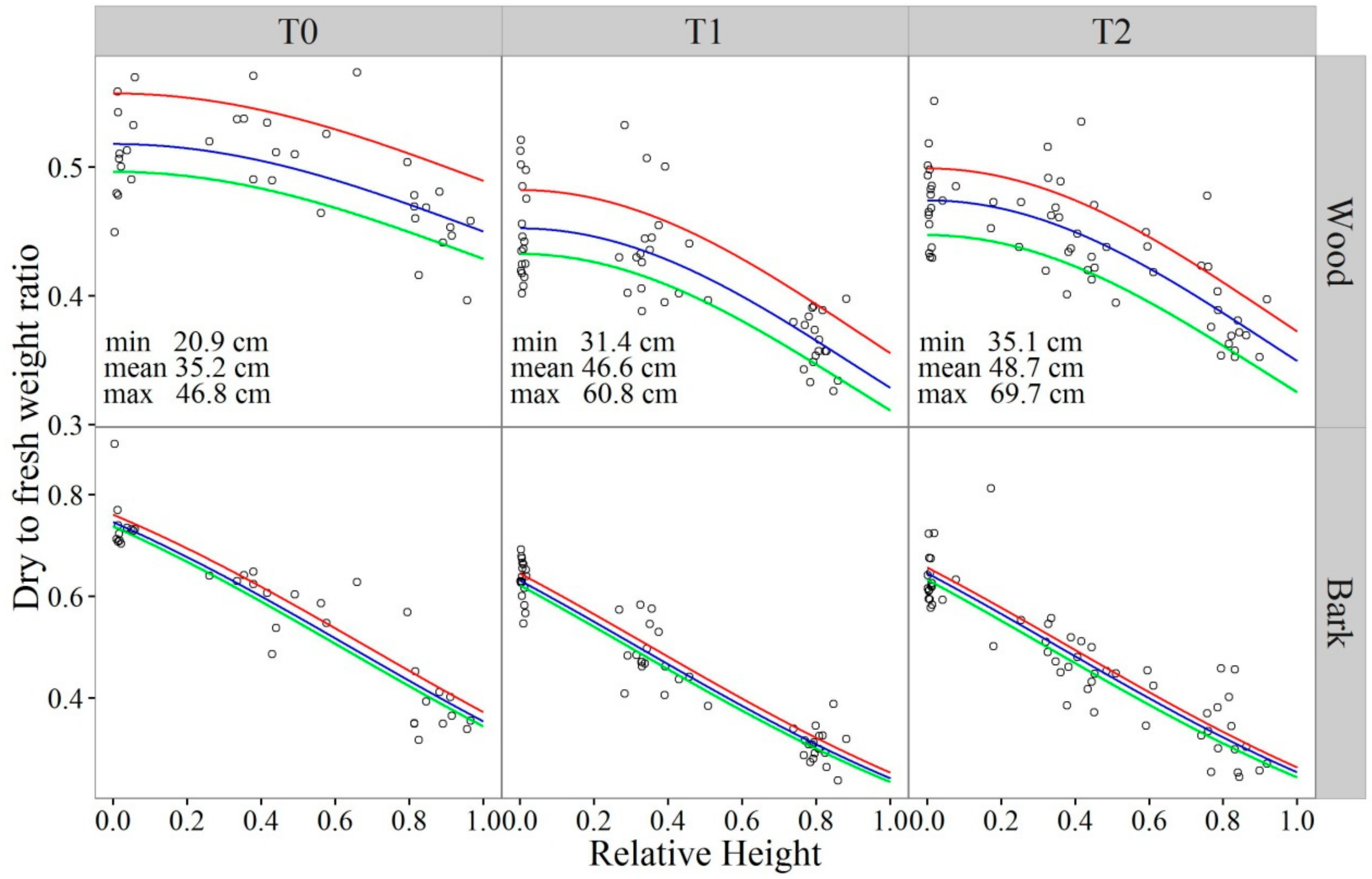
3.1. Dry to Fresh Weight Ratios

The dry to fresh weight ratio of stemwood (${\theta }_w$) varied not only within a tree but also among trees of difference sizes in the same stand and across the three stand types (Figure 3). It decreased systematically from the butt and lower stem, through the mid and upper stem to the top of the tree. The beta regression model in Equation (1) explained about 74% of the variation in logit transformed ${\theta }_w$ among the sample disks as indicated by the value of the pseudo-${\mathrm{R}}^2$ in

Table 2. Estimated parameters, their standard errors (SE) and pseudo-R² of the dry to fresh weight ratio Equations (1) and (2) which were fitted using beta regression for stemwood and bark.

Stemwood			Bark
Parameter	Estimate	SE	Parameter	Estimate	SE
w1	0.4497	0.2009	b1	1.1161	0.3867
w2	0.1063	0.0595	b2	0.0696	0.0438
w3	0.4290	0.0607	b3	0.4982	0.0584
w4	0.5233	0.0540	b4	−1.6781	0.0591
w5	−0.0054	0.0759	b5	−0.1512	0.1008
w6	−0.2514	0.0785
w7	−0.3031	0.0513
pseudo-R2	0.74		pseudo-R2	0.88

. The estimated value of ${\mathrm{w}}_7$, the parameter associated with the log transformed DBHOB in Equation (1), was negative, indicating that large trees tended to have smaller dry to fresh weight ratios. The estimated values of the first three parameters in Equation (1) showed that the ratio was much higher for unthinned stands than for the thinned stands and it was similar between the T1 and T2 stands. As depicted by the curves in Figure 3, the estimated ratio was the highest when relative height (RH) was zero i.e., at ground level. It ranged between 0.50 and 0.56 for unthinned (T0) stands, between 0.43 and 0.48 for T1 stands, and between 0.45 and 0.50 for T2 stands as the DBHOB of the moisture content sample trees decreased from 47 to 21 cm, from 61 to 31 cm and from 70 to 35 cm in the three types of stands respectively.

Like stemwood, the dry to fresh weight ratio of bark (${\theta }_b$) varied along the stem, among trees of difference sizes in the same stand and across the three stand types (Figure 3). It also decreased with RH but more rapidly in a closer to linear way. The beta regression model in Equation (2) explained about 88% of the variation in the observed logit transformed data as indicated by the value of the pseudo-${\mathrm{R}}^2$ in Table 2. The estimated values of the first three parameters in Equation (2) showed that ${\theta }_b$ was also much higher for unthinned (T0) stands than for the thinned stands, but it was about the same for T1 and T2 stands. The ratio also decreased as tree size increased, but to a much less extent in comparison to that of stemwood (Figure 3). Corresponding to the curves for stemwood in Figure 3, the estimated ${\theta }_b$ at RH = 0 ranged between 0.74 and 0.76 for unthinned (T0) stands, between 0.62 and 0.64 for T1, and between 0.63 and 0.66 for T2 stands as the DBHOB of the moisture content sample trees decreased. At RH = 0.5, the corresponding range decreased to 0.55 to 0.58, 0.41 to 0.44 and 0.43 to 0.45 for the T0, T1 and T2 stands respectively. When RH reached 0.95, the range became 0.36 to 0.39, 0.25 to 0.27 and 0.26 to 0.28 for the three respective stand types (Figure 3).

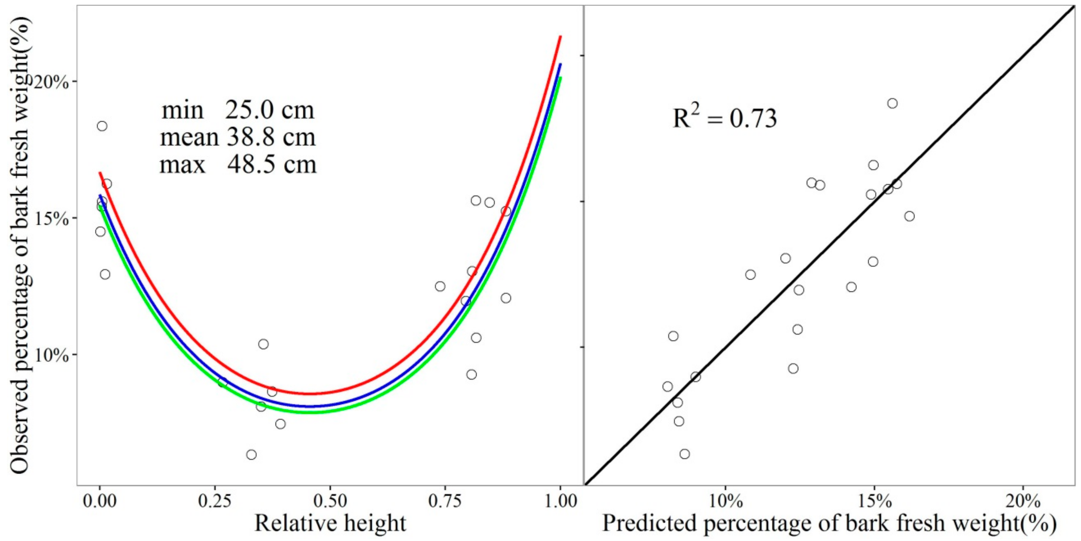
3.2. The Percentage of Bark in the Total Fresh Weight of a Stem Cross-Section

The observed percentage of bark fresh weight of the sample disks varied from 6% to 18% among the disk samples. It initially decreased with RH to reach a minimum about mid stem and then became increasingly larger as RH further increased from mid stem to the tip of the tree (Figure 4). The beta regression model in Equation (3) explained about 73% of the variation in the observed logit transformed data as indicated by the value of the pseudo-${\mathrm{R}}^2$ in

Table 3. Estimated parameters, their standard errors (SE) and pseudo-R² of the percentage of bark fresh weight Equation (3) that was fitted using beta regression.

Parameter	Estimate	SE	Pseudo-R2
a	−1.1667	0.7349	0.73
b	−3.3327	0.4540
c	3.6565	0.5137
d	−0.1374	0.1981

. As depicted by the curves in Figure 4, the estimated percentage of bark at RH = 0 ranged from 15% to 17% as the DBHOB of sample trees decreased from 49 to 25 cm. The range reached its minimum of 8% to 9% at about mid stem when RH = 0.46 and became 17 to 19% at RH = 0.95, close to the tip of the tree (Figure 4).

3.3. Converting Fresh Weight to Dry Weight

Total tree fresh weight ranged from 200 to 5285 kg among the 239 sample trees as their DBHOB varied from 18.0 to 70.1 cm (Figure 2). It had a much narrower range, between 200 and 2633 kg, for unthinned stands where the largest sample tree had a DBHOB of 50.2 cm. Sample trees from T1 and T2 stands had similar ranges of tree size and total tree fresh weight. The converted total tree dry weight varied from 112 to 2249 kg among the 239 sample trees over the same range of tree size, but it fell into a much narrower range of 112 to 1253 kg for unthinned stands.

3.4. Additive Biomass Equations

The estimated values of ${\beta }_{11},$ the exponent of D for product biomass in the four systems of equations (Equations (6), (8), (9) and (10)), varied from 2.06 to 2.30 for fresh weight and from 1.89 to 2.09 for dry weight (

Table 4. Estimated parameters, their standard errors (SE) and R² for the four systems of additive equations for fresh and dry weight prediction. The one-variable model used DBHOB as the only predictor and the two-variable model involved both DBHOB and total tree height. ${\widehat{Y}}_{prod}$ and ${\widehat{Y}}_{res}$ represent the predicted values of $Y_{prod}$ and $Y_{res}$. For all systems of equations in the table, ${\widehat{Y}}_{total}={\widehat{Y}}_{prod}+{\widehat{Y}}_{res}$, i.e., the predicted value of total tree biomass is equal to the sum of the predicted values of its components.

Tree	Parameter	Fresh Weight			Dry Weight
Component		Estimate	SE	R2	Estimate	SE	R2
Equation (6), ${\widehat{Y}}_{prod}={\mathsf{\beta }}_{10}{D}^{{\mathsf{\beta }}_{11}}$, ${\widehat{Y}}_{res}={\mathsf{\beta }}_{20}{D}^{{\mathsf{\beta }}_{21}}$
Product ($Y_{prod}$)	${\mathsf{\beta }}_{10}$	0.2587	0.0283	0.92	0.2761	0.0455	0.90
	${\mathsf{\beta }}_{11}$	2.2997	0.0288		2.0817	0.0433
Residue ($Y_{res})$	${\mathsf{\beta }}_{20}$	0.0255	0.0122	0.60	0.0386	0.0191	0.51
	${\mathsf{\beta }}_{21}$	2.5203	0.1257		2.1674	0.1295
Total ($Y_{total}$)				0.94			0.93
Equation (8), ${\widehat{Y}}_{prod}={\mathsf{\beta }}_{10}{D}^{{\mathsf{\beta }}_{11}}{H}^{{\mathsf{\beta }}_{12}}$, ${\widehat{Y}}_{res}={\mathsf{\beta }}_{20}{D}^{{\mathsf{\beta }}_{21}}$
Product ($Y_{prod}$)	${\mathsf{\beta }}_{10}$	0.0370	0.0117	0.93	0.0378	0.0103	0.92
	${\mathsf{\beta }}_{11}$	2.1122	0.0400		1.8930	0.0505
	${\mathsf{\beta }}_{12}$	0.7740	0.1086		0.7880	0.1012
Residue ($Y_{res})$	${\mathsf{\beta }}_{20}$	0.0248	0.0103	0.60	0.0372	0.0169	0.51
	${\mathsf{\beta }}_{21}$	2.5275	0.1077		2.1755	0.1190
Total ($Y_{total}$)				0.95			0.94
Equation (9), ${\widehat{Y}}_{prod}={\mathsf{\beta }}_{10}{D}^{\left({\mathsf{\beta }}_{11}+{\mathsf{\beta }}_{\mathrm{d}11}{T}_2+{\mathsf{\beta }}_{\mathrm{d}12}{T}_0\right)}$, ${\widehat{Y}}_{res}={\mathsf{\beta }}_{20}{D}^{\left({\mathsf{\beta }}_{21}+{\mathsf{\beta }}_{\mathrm{d}21}{T}_2+{\mathsf{\beta }}_{\mathrm{d}22}{T}_0\right)}$
Product ($Y_{prod}$)	${\mathsf{\beta }}_{10}$	0.3543	0.0406	0.93	0.2535	0.0443	0.92
	${\mathsf{\beta }}_{11}$	2.2140	0.0297		2.0922	0.0461
	${\mathsf{\beta }}_{\mathrm{d}11}$	0.0148	0.0034		0.0223	0.0042
	${\mathsf{\beta }}_{\mathrm{d}12}$	−0.0175	0.0062		0.0171	0.0051
Residue ($Y_{res})$	${\mathsf{\beta }}_{20}$	0.0310	0.0163	0.62	0.0392	0.0176	0.51
	${\mathsf{\beta }}_{21}$	2.4914	0.1353		2.1606	0.1163
	${\mathsf{\beta }}_{\mathrm{d}21}$	−0.0359	0.0136
	${\mathsf{\beta }}_{\mathrm{d}22}$	−0.0404	0.0242
Total ($Y_{total}$)				0.95			0.94
Equation (10), ${\widehat{Y}}_{prod}={\beta }_{10}{D}^{\left({\mathsf{\beta }}_{11}+{\mathsf{\beta }}_{\mathrm{d}11}{T}_2+{\mathsf{\beta }}_{\mathrm{d}12}{T}_0\right)}{H}^{{\mathsf{\beta }}_{12}}$, ${\widehat{Y}}_{res}={\mathsf{\beta }}_{20}{D}^{\left({\mathsf{\beta }}_{21}+{\mathsf{\beta }}_{\mathrm{d}21}{T}_2+{\mathsf{\beta }}_{\mathrm{d}22}{T}_0\right)}$
Product ($Y_{prod}$)	${\mathsf{\beta }}_{10}$	0.0516	0.0168	0.94	0.0326	0.0086	0.93
	${\mathsf{\beta }}_{11}$	2.0562	0.0449		1.9163	0.0495
	${\mathsf{\beta }}_{12}$	0.7339	0.1198		0.7900	0.0958
	${\mathsf{\beta }}_{\mathrm{d}11}$	0.0148	0.0036		0.0228	0.0037
	${\mathsf{\beta }}_{\mathrm{d}12}$	−0.0114	0.0068		0.0262	0.0051
Residue ($Y_{res})$	${\mathsf{\beta }}_{20}$	0.0295	0.0136	0.62	0.0374	0.0148	0.51
	${\mathsf{\beta }}_{21}$	2.5040	0.1186		2.1722	0.1019
	${\mathsf{\beta }}_{\mathrm{d}21}$	−0.0359	0.0123
	${\mathsf{\beta }}_{\mathrm{d}22}$	−0.0399	0.0241
Total ($Y_{total}$)				0.95			0.95

). In comparison, the estimated values of ${\mathsf{\beta }}_{21}$, the exponent of D for residue biomass in the four systems of equations, varied from 2.49 to 2.52 for fresh weight and from 2.16 to 2.18 for dry weight. The estimates of ${\mathsf{\beta }}_{\mathrm{d}11}$ for dummy variable T2 in Equations (9) and (10) for product fresh weight were small positive values but significantly greater than the estimates of ${\mathsf{\beta }}_{\mathrm{d}12}$ for unthinned stands. For product dry weight, the differences between the two parameter estimates became much smaller and non-significant. The estimates of ${\mathsf{\beta }}_{\mathrm{d}21}$ and ${\mathsf{\beta }}_{\mathrm{d}22}$ in Equation (9) for residue fresh weight were similar to those in Equation (10). The estimates of ${\mathsf{\beta }}_{12}$, the exponent of H in Equations (8) and (10) for product biomass, varied narrowly between 0.73 and 0.79 among the equations for both fresh and dry weight. The value of ${\mathrm{R}}^2$ ranged between 0.92 to 0.94 for product fresh weight and between 0.90 and 0.93 for product dry weight among the four systems of equations. It varied between 0.60 and 0.62 for residue fresh weight and was 0.51 for residue dry weight. As expected, the value of ${\mathrm{R}}^2$ was the highest for total tree biomass than for the product and residue components in all fresh and dry weight equations (Table 4).

The estimates of b, the exponent of $\widehat{Y}$ in the residual variance function Equations (14) and (15), ranged from 1.36 to 1.70 for residue fresh and dry weight among the four systems of equations (

Table 5. Estimated scale factors ${\widehat{\mathit{\sigma }}}_{}^2$ and exponents of the residual variance functions for product, residue and total tree fresh and dry weight predicted by the system of additive equations without the incorporation of dummy variables for stand types, firstly using D as the independent variable (Equation (6)) and secondly using D and H as the predictors (Equation (8)). θ_s is Snowdon’s bias correction factor, p₅ and p₉₅ are the fifth and ninety-fifth percentiles of the weighted residuals.

Tree Component	Predictor	${\widehat{\mathit{\sigma }}}_{}^2{\widehat{\mathit{Y}}}^{\mathit{b}}$		${\mathit{\theta }}_{\mathit{s}}$	p5	p95
		${\widehat{\mathit{\sigma }}}_{}^2$	b
Fresh weight
D	15.3344	0.8764	5.1923	−1.6947	1.3512
Residue	D	0.3872	1.6312	3.5267	−1.3098	1.6301
Total	D	0.1950	1.4607	3.9601	−1.6560	1.5318
Dry weight
Product	D	1.3190	1.1296	4.7699	−1.7473	1.3031
Residue	D	0.9646	1.4208	3.4076	−1.1757	1.8415
Total	D	1.1391	1.1534	3.8866	−1.5161	1.3727
Fresh weight
Product	D, H	10.7596	0.9171	4.5895	−1.5781	1.2667
Residue	D, H	0.4047	1.6220	3.5703	−1.3150	1.6298
Total	D, H	0.2604	1.4009	4.0150	−1.4839	1.6155
Dry weight
Product	D, H	7.6822	0.8563	4.3787	−1.5936	1.3505
Residue	D, H	1.0377	1.4068	3.4324	−1.1673	1.8546
Total	D, H	0.0919	1.4749	4.2767	−1.5239	1.4914

,

Table 6. Estimated scale factors ${\widehat{\mathit{\sigma }}}_{}^2$ and exponents of the residual variance functions for product, residue and total tree fresh and dry weight predicted by the system of additive equations with the incorporation of dummy variables for stand types, using D as the independent variable (Equation (9)). θ_s is Snowdon’s bias correction factor, p₅ and p₉₅ are the fifth and ninety-fifth percentiles of the weighted residuals.

Tree Component	Stand	${\widehat{\mathit{\sigma }}}_{}^2{\widehat{\mathit{Y}}}^{\mathit{b}}$		θs	p5	p95
	Type	${\widehat{\mathit{\sigma }}}_{}^2$	b
Fresh weight
Product	T0	6.7815	0.9458	4.4141	−1.6618	1.5271
	T1	9.7562	0.9458	5.6492	−1.5033	1.3586
	T2	7.3155	0.9458	4.6826	−1.3650	1.5189
Residue	T0	0.3675	1.7025	2.6791	−1.0969	1.6872
	T1	0.1773	1.7025	4.3380	−1.3152	1.6022
	T2	0.2290	1.7025	3.7288	−1.2699	1.8052
Total	T0	0.0588	1.6768	2.3100	−1.8942	1.3194
	T1	0.0475	1.6768	3.1247	−1.4882	1.4235
	T2	0.0328	1.6768	3.6697	−1.8579	1.7139
Dry weight
Product	T0	3.4018	0.9605	3.6655	−1.8418	1.3759
	T1	3.8532	0.9605	5.5436	−1.6111	1.1995
	T2	3.1352	0.9605	4.1343	−1.2882	1.6791
Residue	T0, T1, T2	1.2607	1.3621	3.5896	−1.1511	1.8664
Total	T0	0.1218	1.5100	2.5433	−1.9707	1.3969
	T1	0.1134	1.5100	3.0902	−1.4408	1.4230
	T2	0.0760	1.5100	3.8888	−1.7484	1.6971

and

Table 7. Estimated scale factors ${\widehat{\mathit{\sigma }}}_{}^2$ and exponents of the residual variance functions for product, residue and total tree fresh and dry weight predicted by the system of additive equations with the incorporation of dummy variables for stand types, using D and H as the independent variables Equation (10). θ_s is Snowdon’s bias correction factor, p₅ and p₉₅ are the fifth and ninety-fifth percentiles of the weighted residuals.

Tree Component	Stand	${\widehat{\mathit{\sigma }}}_{}^2{\widehat{\mathit{Y}}}^{\mathit{b}}$		${\mathit{\theta }}_{\mathit{s}}$	p5	p95
	Type	${\widehat{\mathit{\sigma }}}_{}^2$	b
Fresh weight
Product	T0	3.3324	1.1226	3.3611	−1.6399	1.2789
	T1	1.9472	1.1226	5.6202	−1.7525	1.2699
	T2	1.8473	1.1226	4.0394	−1.4824	1.4159
Residue	T0	0.4529	1.6645	2.6948	−1.0964	1.6950
	T1	0.2260	1.6645	4.3267	−1.3056	1.5984
	T2	0.2765	1.6645	3.9167	−1.2788	1.8020
Total	T0	0.0042	2.0262	3.0365	−1.8946	1.3323
	T1	0.0023	2.0262	3.2479	−1.8056	1.6948
	T2	0.0021	2.0262	2.9956	−1.5580	1.6932
Dry weight
Product	T0	5.7190	0.9349	3.5573	−1.8767	1.0616
	T1	3.0913	0.9349	5.9595	−1.6808	1.1194
	T2	3.5089	0.9349	3.5960	−1.3641	1.5202
Residue	T0, T1, T2	1.2744	1.3586	3.6255	−1.1495	1.8714
Total	T0	0.0078	1.9280	2.9966	−2.0387	1.3830
	T1	0.0040	1.9280	3.4928	−1.8257	1.6743
	T2	0.0035	1.9280	3.3492	−1.4458	1.6745

). They were much greater than the estimates for product fresh and dry weight which varied from 0.86 to 1.13 across the four systems of equations. Correspondingly, the spread of residuals about $\widehat{Y}$ as delineated by Equation (16) expanded much faster for residue than for product fresh and dry weight across all systems of equations as $\widehat{Y}$ increased (Figure 5). Comparing to Equations (6) and (9) where diameter was the only independent variable, the incorporation of H as an additional predictor in Equations (8) and (10) led to slightly narrower confidence bands for product biomass but not so for residue biomass. For Equations (9) and (10) where dummy variables were used to represent stand types, the confidence bands that contained approximately 90% of the observed data of product, residue and total tree fresh weight were wider for T1 stands than for the other two stand types as shown by graphical plotting of the residual variance functions in Table 6 and Table 7.

3.5. Allocative Biomass Equations

The 36 trees that produced sawlogs only but not any pulpwood represented 15% of all the trees that were destructively sampled. An extensive exploratory analysis suggested that the occurrence of these trees could be regarded as at random because it did not relate to or associate with any tree and stand attributes including DBHOB, total tree height, stand type and particular plots or sites.

Four sets of parameter estimates were obtained for each of the two systems of allocative equations (Equations (12) and (13)) using the predicted product and residue fresh weight from Equations (6), (8), (9) and (10) respectively. Similarly, another four sets of parameter estimates were obtained using the predicted product and residue dry weight from the four equations. For both fresh and dry weight, there were very small and practically negligible differences among the four equations in the proportional allocation of product biomass to its sawlog and pulpwood components and in the proportional allocation of residue biomass to its stump, branch and waste components for a given value of DBHOB. For the sake of parsimony, the parameters of the two allocative systems of equations estimated using the predicted product and residue biomass from Equation (10) were reported in this paper (

Table 8. Estimated parameters, their standard errors (SE) and R² for the two systems of allocative equations (Equations (12) and (13)) for product and residue fresh and dry weight as displayed in the footnote. All variables with a hat in the footnote denote the predicted values of biomass components that they represent.

Equation (12): ${\widehat{Y}}_{saw}=\frac{1}{1+{\mathrm{r}}_{11}{D}^{{\mathrm{r}}_{12}}}{\widehat{Y}}_{prod}$, ${\widehat{Y}}_{pulp}=\frac{{\mathrm{r}}_{11}{D}^{{\mathrm{r}}_{12}}}{1+{\mathrm{r}}_{11}{D}^{{\mathrm{r}}_{12}}}{\widehat{Y}}_{prod}$; Equation (13): ${\widehat{Y}}_{stump}=\frac{1}{1+{\mathrm{r}}_{21}{D}^{{\mathrm{r}}_{22}}+{\mathrm{r}}_{23}{D}^{{\mathrm{r}}_{24}}}{\widehat{Y}}_{res}$, ${\widehat{Y}}_{branch}=\frac{{\mathrm{r}}_{21}{D}^{{\mathrm{r}}_{22}}}{1+{\mathrm{r}}_{21}{D}^{{\mathrm{r}}_{22}}+{\mathrm{r}}_{23}{D}^{{\mathrm{r}}_{24}}}{\widehat{Y}}_{res}$, ${\widehat{Y}}_{waste}=\frac{{\mathrm{r}}_{23}{D}^{{\mathrm{r}}_{24}}}{1+{\mathrm{r}}_{21}{D}^{{\mathrm{r}}_{22}}+{\mathrm{r}}_{23}{D}^{{\mathrm{r}}_{24}}}{\widehat{Y}}_{res}$.

).

Using these parameter estimates in Equations (12) and (13), the predicted allocation of total product biomass to sawlogs increased from 83% to 85% in fresh weight and from 82% to 87% in dry weight and that to pulpwood decreased from 17% to 15% in fresh weight and 18% to 13% in dry weight as DBHOB increased from 15 to 70 cm (

Table 9. Fractions of the sub-components in the product and residue fresh and dry weight as predicted by the two systems of allocative Equations (12) and (13) using the parameter estimates in Table 8.

DBHOB (cm)	Product		Residue
	Sawlog	Pulpwood	Stump	Branch	Waste
Fresh weight
15	0.8283	0.1717	0.1074	0.1797	0.7129
20	0.8329	0.1671	0.1112	0.2467	0.6421
25	0.8363	0.1637	0.1117	0.3088	0.5794
30	0.8391	0.1609	0.1104	0.3651	0.5244
35	0.8414	0.1586	0.1081	0.4157	0.4763
40	0.8434	0.1566	0.1051	0.4608	0.4341
45	0.8452	0.1548	0.1017	0.5011	0.3972
50	0.8467	0.1533	0.0983	0.5370	0.3647
55	0.8481	0.1519	0.0949	0.5690	0.3361
60	0.8494	0.1506	0.0915	0.5978	0.3108
65	0.8505	0.1495	0.0882	0.6235	0.2883
70	0.8516	0.1484	0.0851	0.6467	0.2682
Dry weight
15	0.8209	0.1791	0.1225	0.1758	0.7017
20	0.8313	0.1687	0.1288	0.2314	0.6398
25	0.8390	0.1610	0.1318	0.2820	0.5862
30	0.8450	0.1550	0.1328	0.3276	0.5396
35	0.8500	0.1500	0.1325	0.3687	0.4988
40	0.8542	0.1458	0.1313	0.4058	0.4629
45	0.8579	0.1421	0.1297	0.4393	0.4311
50	0.8611	0.1389	0.1276	0.4696	0.4028
55	0.8639	0.1361	0.1254	0.4971	0.3775
60	0.8664	0.1336	0.1231	0.5221	0.3548
65	0.8687	0.1313	0.1207	0.5450	0.3344
70	0.8708	0.1292	0.1182	0.5659	0.3158

). The predicted allocation of total residue biomass to stump varied between 9% and 11% in fresh weight and between 12% and 13% in dry weight over the diameter range. In comparison, the predicted allocation of total residue biomass to branches increased from 18% to 65% in fresh weight and from 18% to 57% in dry weight, and that to waste decreased from 71% to 27% in fresh weight and from 70% to 32% in dry weight. Among the five subcomponents, the residual variation about the predicted values was comparatively larger for pulpwood and waste as their ${\mathrm{R}}^2$ values were less than 0.3 and 0.15 respectively (Table 8).

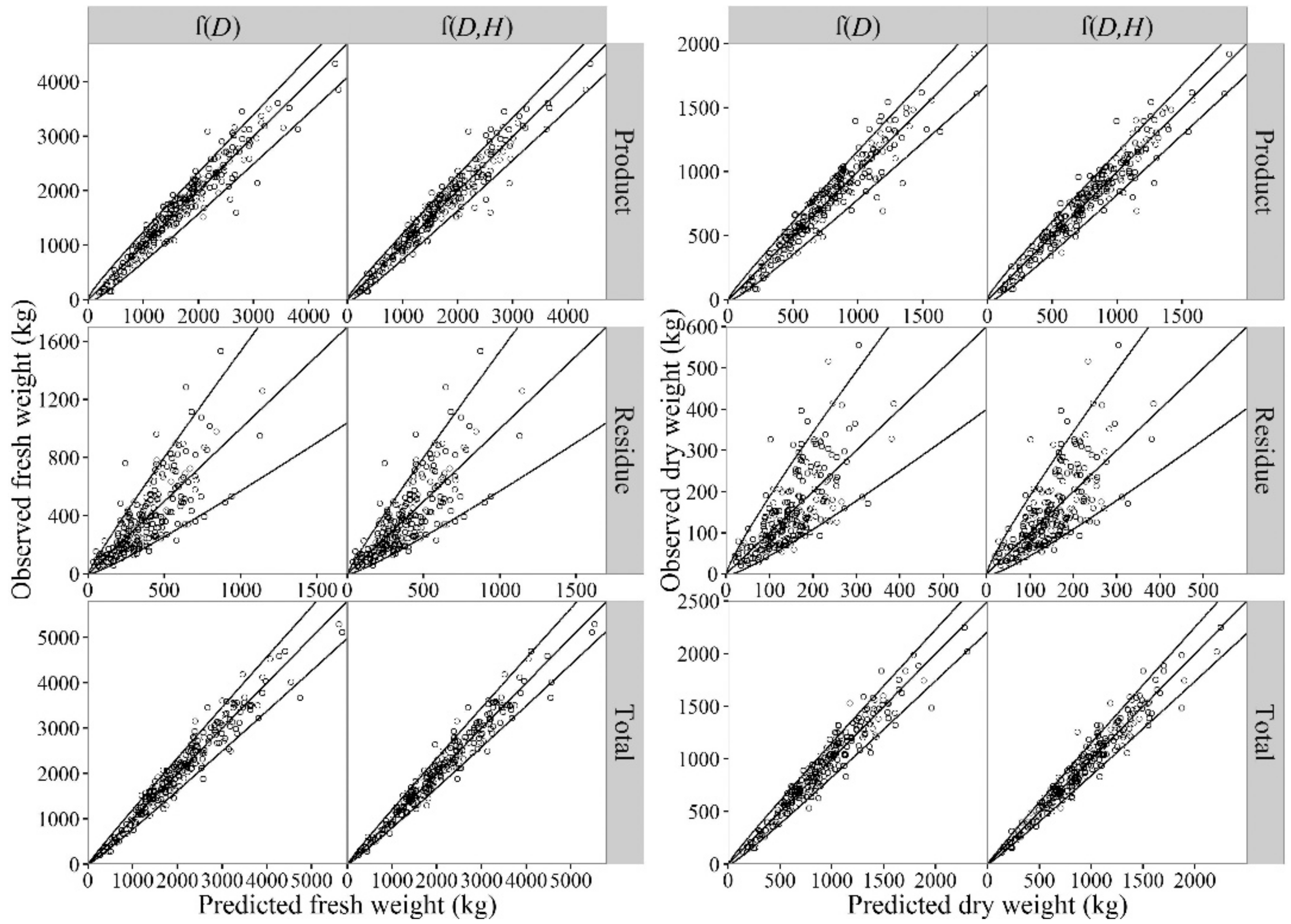
3.6. Prediction Accuracy

The MEP from the leave-one-plot-out cross-validation was very small for the product, residue and total tree biomass in both fresh and dry weight across all four systems of additive equations (

Table 10. Benchmarking statistics for component and total tree fresh and dry weight predictions calculated following the leave-one-plot-out cross-validation procedure: the mean error of prediction (MEP), the mean percentage error of prediction (MPEP), the mean absolute error of prediction (MAEP), the mean percentage absolute error of prediction (MPAEP) and the mean squared error of prediction (MSEP).

Tree	Fresh Weight						Dry Weight
Component	MEP (kg)	MPEP (%)	MAEP (kg)	MPAEP (%)	MSEP	${\mathbf{R}}_{\mathbf{p}}^2$	MEP (kg)	MPEP (%)	MAEP (kg)	MPAEP (%)	MSEP	${\mathbf{R}}_{\mathbf{p}}^2$
Equation (6), one-variable model, without dummy variable
Product	−2.4	−1.5	167.7	11	57,964	0.91	−0.3	−1.3	79.7	11	13,146	0.89
Residue	0.1	1.8	120.6	33	27,043	0.58	0.1	1.8	49.4	35	4439	0.49
Total	−2.3	−1.1	181.0	9	61,220	0.94	−0.2	−0.9	82.5	10	12,908	0.92
Sawlog	9.6	−1.8	216.4	18	83,420	0.84	4.2	−1.5	98.9	17	17,690	0.82
Pulpwood	4.4	6.2	140.6	58	41,820	0.25	2.1	6.0	62.9	61	8269	0.18
Stump	−0.3	−1.9	9.0	24	188	0.60	−0.1	−1.2	4.6	25	46	0.57
Branch	−3.4	1.0	63.7	33	8529	0.63	−1.4	1.3	20.5	32	838	0.62
Waste	3.8	4.6	100.1	68	18,990	0.13	1.6	4.3	44.1	71	3645	0.09
Equation (8), two-variable model, without dummy variable
Product	−1.5	−1.1	155.8	10	48,356	0.93	0.0	−0.8	74.9	11	11,005	0.91
Residue	−0.5	1.8	120.5	33	27,000	0.58	0.6	2.2	49.3	35	4435	0.49
Total	−2.1	−0.6	166.7	9	51,909	0.95	0.6	−0.3	74.9	9	10,724	0.94
Sawlog	10.4	−1.5	203.7	17	75,537	0.85	4.4	−1.2	93.0	16	15,845	0.84
Pulpwood	4.7	8.0	142.3	60	41,976	0.25	2.2	7.9	63.7	63	8315	0.18
Stump	−0.4	−1. 9	9.0	24	188	0.60	−0.1	−0.8	4.5	25	46	0.57
Branch	−3.8	1.0	63.7	33	8511	0.64	−1.1	1.7	20.4	32	836	0.62
Waste	3.6	4.6	100.1	68	18,986	0.13	1.8	4.7	44.1	72	3645	0.09
Equation (9), one-variable model, with dummy variables
Product	−2.3	−1.3	163.0	11	53,112	0.92	−2.8	−1.4	74.4	11	10,924	0.91
Residue	−0.1	2.2	118.9	33	26,172	0.60	1.3	2.6	49.3	35	4466	0.49
Total	−2.4	−0.9	179.6	9	60,194	0.94	−1.5	−0.9	79.5	9	11,409	0.93
Sawlog	10.6	−1.5	208.1	17	78,969	0.84	2.5	−1.6	95.8	17	16,226	0.83
Pulpwood	4.7	6.4	140.3	58	41,393	0.26	1.8	6.0	62.7	61	8164	0.19
Stump	−0.3	−1.3	9.4	25	197	0.59	−0.1	−1.4	4.6	25	46	0.57
Branch	−3.3	0.9	60.5	33	7388	0.68	0.1	2.5	20.3	32	832	0.63
Waste	3.6	5.6	101.6	69	19,361	0.11	1.3	4	44.2	72	3636	0.09
Equation (10), two-variable model, with dummy variables
Product	−3.7	−1.0	152.2	10	45,046	0.93	−3.9	−1.2	68.4	10	9036	0.92
Residue	0.6	2.6	118.8	33	26,159	0.60	1.9	3.1	49.2	35	4462	0.49
Total	−3.1	−0.6	166.2	9	51,575	0.95	−1.9	−0.6	71.6	8	9395	0.94
Sawlog	9.5	−1.3	199.5	17	73,535	0.85	1.6	−1.6	90.8	16	14,813	0.85
Pulpwood	4.6	8.0	141.5	60	41,439	0.26	1.7	7.4	63.5	63	8198	0.19
Stump	−0.3	−1.0	9.4	25	197	0.59	0.0	−1.0	4.6	25	46	0.57
Branch	−3.0	1.3	60.4	33	7366	0.68	0.4	3.0	20.3	32	831	0.63
Waste	3.9	6.0	101.5	70	19,368	0.11	1.6	4.8	44.2	72	3635	0.09

). The MPEP for product and total tree biomass lied between −1.5% and −0.3%, but that for residue biomass was slightly larger, falling between 1.8% and 3.1%. The MPAEP was 10 to 11% for product, 33 to 35% for residue and 8 to 10% for total tree biomass predictions. The values of ${\mathrm{R}}_{\mathrm{p}}^2$ for product and total tree biomass prediction were mostly between 0.91 and 0.95, and that for residue biomass were much lower, in the range of 0.49 to 0.60. In comparison to the four systems of additive equations, the MEP was larger for the two allocative systems of equations. The MPEP was between −1.8% and −1.2% for sawlog biomass, between 6.0% and 8.0% for pulpwood biomass, between −1.9% and −0.8% for stump biomass, between 0.9% and 3.0% for branch biomass, and between 4.0% and 6.0% for waste biomass in fresh and dry weight (Table 10). The MPAEP was 16% to 18% for sawlog, 58 to 63% for pulpwood, 24% to 25% for stump, 32 to 33% for branch, 68 to 72% for waste biomass in fresh as well as dry weight. The values of ${\mathrm{R}}_{\mathrm{p}}^2$ were 0.82 to 0.85 for sawlog, 0.18 to 0.26 for pulpwood, 0.57 to 0.60 for stump, 0.62 to 0.68 for branch and 0.09 to 0.13 for waste biomass prediction. In general, ${\mathrm{R}}_{\mathrm{p}}^2$ was higher for fresh weight than for dry weight predictions across all additive and allocative equations.

In comparison with Equation (6) where D was the only predictor, including total tree height as an additional predictor in Equation (8) resulted in a 15 to 17% reduction in MSEP for product and total tree biomass prediction, 9 to 10% reduction in the MSEP for sawlog biomass prediction in both fresh and dry weight, and almost no reduction for all other components (Table 10). Incorporating dummy variables for stand types in Equation (9) led to a reduction in the MSEP of 8% and 17% for product fresh and dry weight predictions, 3% and −1% for residue, 2% and 12% for total tree, 5% and 8% for sawlog, 13% and 0% for branch fresh and dry weight predictions. The reduction in the MSEP for other components (i.e., pulpwood, stump and waste) was generally less than 3%. When both total tree height and dummy variables were incorporated in Equation (10) as predictors, the reduction in the MSEP was 22% and 31% for product fresh and dry weight predictions, 3% and −1% for residue, 16% and 27% for total tree, 12% and 16% for sawlog, 14% and 1% for branch fresh and dry weight predictions. For stump and waste fresh weight, the MSEP was slightly larger, but for their dry weight, it had little or no reduction.

4. Discussion

It has long been recognised that there is a systematic variation of moisture content in the wood of living trees (e.g., [18,78,79,80]). Such variations would have implications on tree-based estimates of biomass [81], and in the case of this study, on the estimation of stem biomass using the dry to fresh wood ratios from disks subsampled from the stems of sample trees in particular. The vertical variation of moisture content in the stemwood of planted P. radiata trees have been well observed for more than 60 years [18,19,45,82]. However, there is still a lack of quantitative models for the systematic variation apart from a simple quadratic function used by Tian et al. [83] to describe the change in basic density of stemwood with height above ground level. Our results showed that this vertical variation in the dry to fresh weight ratio of stemwood could best be modelled by a cosine curve between zero and $\frac{\pi }{2}$ over the whole stem from ground to tip with a logit link function through beta regression as in Equation (1). As relative height (RH) increased from zero to one, i.e., from ground level to the tip of the tree, the estimated dry to fresh weight ratio decreased from a maximum to a minimum value that were determined by the estimated parameters in the equation (Figure 3). The pattern of change also varied with stand type and tree size in a way consistent with that previously reported by Fielding [18] and Moreno Chan [82] for plantation-grown P. radiata in Australia. The former showed that the moisture content increased with height above ground within a tree and large dominant trees tended to have higher moisture content than the small suppressed ones. The latter found that the green sapwood of rotation age trees in unthinned stands had lower moisture content than that of trees in thinned stands and the moisture content also increased with height above around. Furthermore, trees in unthinned stands had consistently lower sapwood percentages than the thinned stands.

Despite the numerous studies on the biomass of P. radiata trees (see [84]), the systematic change in the moisture content of bark along the stem from ground to tip has not been modelled as far as the literature we reviewed. The model specified in Equation (2) not only served as a good starting point for doing so but also linked the systematic change to stand type and tree size. The dry to fresh weight ratio of bark decreased more rapidly and covered a wider range than that of stemwood as RH increased (Figure 3). The pattern of change varied with stand type, with trees in unthinned stands having drier bark than in thinned stands, and it also varied with tree size, but to a lesser extent as suggested by the ratio of parameter estimate associated with D and its standard error in Table 2. In comparison to Equation (2), Equation (3) for describing the fraction of bark in the total fresh weight of a stem cross-section was estimated with a much smaller number of sample disks from nine trees. The U-shaped pattern of change in the estimated fraction of bark fresh weight with increasing RH was consistent with the findings for mature P. radiata reported in Young et al. [85] and Murphy and Crown [86] and with the log weight data before and after debarking used in Ximenes et al. [45]. The estimated percentages of bark fresh weight along the stem of trees as depicted by the curves in Figure 4 were also within the range of previously reported or obtained data. They were higher than the 7 to 8% reported for mature trees in New Zealand [85,86], but somewhat lower than the values calculated using the log weight data of Ximenes et al. [45]. The data contained a total of 149 logs from 54 sample trees with DBHOB ranging from 36 to 55 cm in Greenhill State Forest of NSW. Each tree was cut into logs about 6 m in length and sequentially coded from butt to top. The logs were then transported to the local sawmill and weighed before and after debarking. The percentage of bark ranged from 10.3% to 18.2% with a median of 15.6% for the butt logs, from 11.1% to 17.3% with a median of 13.9% for the second logs, from 12.5% to 18.6% with a median of 15.0% for the third logs and from 16.1% to 22.3% with a median of 19.2% for the top logs. The inevitable loss of some moisture from logs during the transportation and weighing process at the local sawmill might lead to slightly higher bark percentages.

The systems of additive and allocative biomass equations developed in this study provided the first example of how the bottom-up and the top down approaches could be used together for the estimation of total tree, major and sub-component biomass. Such a combined use of the two approaches is particularly useful when a sub-component is not always present in a major component, leading to unbalanced data where the number of observations is not the same for all equations. In the case of this study, 15% of the sample trees produced sawlogs only, leaving 36 trees without the pulpwood subcomponent for product biomass. In such cases, it is presently problematic or impossible to estimate both major and sub-components in one system of additive biomass equations with cross-equational parameter constraints through seemingly unrelated regression without any loss of information, although some progress in this regard has been made in econometrics [87,88]. This problem was avoided by developing additive equations for the major components first and then breaking each major component into subcomponents through allocative biomass equations. However, when the systems of additive and allocative equations are used together to estimate the biomass of all components of individual trees, random numbers need to be generated from the binomial distribution with $p=0.15$ to set aside trees for producing sawlogs only.

For all systems of additive equations, the fitting statistics, the estimated residual variance and skedastic functions and the benchmarking statistics from the leave-one-plot-out cross-validation showed that product and total tree biomass could be estimated with a much higher degree of accuracy than residue biomass. The systems of equations explained over 90% of the variations in product and total tree biomass, but only about 60% and 50% of the variations in residue dry and fresh weight (Table 4 and Table 10). Including total tree height as an additional predictor in the systems of equations made no improvement in the accuracy of residue biomass prediction. Incorporating dummy variables for stand types led to a small improvement for residue fresh weight but not for dry weight prediction. However, the percentage of residue in the predicted total tree fresh and dry weight differed slightly among the three stand types. Based on the predicted values from Equation (9), the percentage of residue fresh weight increased from 14.8% to 20.5%, from 15.6% to 22.2%, from 13.9% to 18.7% for trees in the unthinned, T1 and T2 stands respectively, as DBHOB increased from 15 to 70 cm. The corresponding changes in the percentage of residue dry weight were from 15.1% to 16.1%, from 15.7% to 17.1%, and from 14.9% to 15.8% for the three stand types. It should be noted that trees in T2 stands had lower percentages of residue biomass than those in unthinned and T1 stands. These percentages were within the broad range of values reported by Madgwick and Webber [44], Ximenes et al. [45] and Cartes-Rodríguez et al. [46] for rotation age P. radiata, although there were some differences in the definition of residue biomass, and in the age and stand conditions among the studies.

The system of allocative equations for product biomass Equation (12) predicted that sawlogs with bark accounted for 83% to 85% of product fresh weight and 82% to 87% of product dry weight over a range of DBHOB from 15 to 70 cm (Table 9). These results were comparable with the range of 80% to 90% over three diameter classes reported by Ximenes et al. [45] for sawlogs without bark harvested from 54 sample trees in Greenhill State Forests of NSW. The predicted allocation of total residue dry weight to stump changed little, between 12% and 13%, over the same diameter range, but it was slightly higher for trees with DBHOB between 30 and 45 cm (Table 9). When these values were converted to percentages of total tree dry weight, they ranged between 1.8% and 2.1% for trees in unthinned stands, between 1.9% and 2.2% for trees in T1 stands, and between 1.8% and 2.0% for trees in T2 stands. The proportion of stump in total tree biomass was 2.1% on average for the 54 trees sampled by Ximenes et al. [45]. The increasing allocation of residue biomass to branches and decreasing allocation to waste as DBHOB increased was expected as larger dominant trees tended to have bigger crowns with large branches. However, it should be kept in mind that there was a great degree of variation in the amount of waste produced during harvesting among individual trees. The system of allocative equations only explained a small part of this variation (Table 10).

The systems of additive and allocative biomass equations developed in this study for individual trees in rotation age P. radiata stands under three thinning regimes represented a significant step forward from the initial preliminary study of Ximenes et al. [45]. They represented a much enhanced capacity to more accurately estimate product and residue biomass of rotation age trees in P. radiata plantations. In addition, the uncertainty associated with the product, residue and total tree biomass were quantified by the residual variance and skedastic functions. These systems of equations can be used together with pre-harvesting inventory data to estimate product and residue biomass at an individual tree level or at a stand level after scaling up. They can also be readily used with harvester data for the spatial mapping of residual biomass once the DBHOB and total height of the harvested stems contained in the harvester data are estimated as in Lu et al. [89]. The current renewable energy target of the Australian Government requires more than 23.5% of Australia’s electricity to be derived from renewable sources by 2020. The target includes biomass as an eligible form of renewable energy generation. This allows harvest residues that would otherwise be burnt or left to rot on the forest floor to generate power and reduce greenhouse gas emissions. The systems of equations will provide forest management with a much enhanced capacity to more accurately estimate product and residue biomass of rotation age trees in P. radiata plantations and thus to include the production of biomass for renewable energy generation in their management systems.

5. Conclusions

Harvest residues in P. radiata plantations have been increasingly recognised and utilized as a source of woody biomass for renewable energy generation in Australia and other major growing countries. However, there is a lack of a systematic approach to the estimation of product and residue biomass and their respective components for individual trees. This study developed four systems of nonlinear additive equations for the estimation of product and residue fresh and dry weight of individual trees in rotation age stands under three thinning regimes. To allocate the predicted product and residue biomass to their respective subcomponents, two systems of allocative equations were developed. Such a combined use of the additive and allocative systems of equations provided the first example of how the two approaches could be used together for the estimation of total tree, major and sub-component biomass. Besides their applications in the management and planning of P. radiata plantations, these systems of equations for individual trees will provide the basis for the further development of stand level systems of equations for product and residue biomass estimation in the future.

References

1. Arnold, J.E.M.; Jongma, J. Fuelwood and charcoal in developing countries. South Asia 1977, 267, 0–38. [Google Scholar]
2. Bhattacharya, S.C.; Salam, P.A. Low greenhouse gas biomass options for cooking in the developing countries. Biomass Bioenergy 2002, 22, 305–317. [Google Scholar] [CrossRef]
3. Flinn, D.W. Comparison of establishment methods for Pinus radiata on a former P. pinaster site. Aust. For. 1978, 41, 167–176. [Google Scholar] [CrossRef]
4. Pye, J.M.; Vitousek, P.M. Soil and nutrient removals by erosion and windrowing at a southeastern U.S. Piedmont site. For. Ecol. Manag. 1985, 11, 145–155. [Google Scholar] [CrossRef]
5. Dyck, W.J.; Beets, P.N. Managing for long-term site productivity. N. Z. For. Nov. 1987, 32, 23–26. [Google Scholar]
6. Creutzig, F.; Ravindranath, N.H.; Berndes, G.; Bolwig, S.; Bright, R.; Cherubini, F.; Chum, H.; Corbera, E.; Delucchi, M.; Faaij, A.; et al. Bioenergy and climate change mitigation: An assessment. Glob. Chang. Biol. Bioenergy 2015, 7, 916–944. [Google Scholar] [CrossRef] [Green Version]
7. Röder, M.; Thornley, P. Bioenergy as climate change mitigation option within a 2 °C target—Uncertainties and temporal challenges of bioenergy systems. Energy Sustain. Soc. 2016, 6, 6–12. [Google Scholar] [CrossRef]
8. Souza, G.M.; Ballester, M.V.R.; De Brito Cruz, C.H.; Chum, H.; Dale, B.; Dale, V.H.; Fernandes, E.C.M.; Foust, T.; Karp, A.; Lynd, L.; et al. The role of bioenergy in a climate-changing world. Environ. Dev. 2017, 23, 57–64. [Google Scholar] [CrossRef]
9. Hoogwijk, M.; Faaij, A.; Van Den Broek, R.; Berndes, G.; Gielen, D.; Turkenburg, W. Exploration of the ranges of the global potential of biomass for energy. Biomass Bioenergy 2003, 25, 119–133. [Google Scholar] [CrossRef]
10. Parikka, M. Global biomass fuel resources. Biomass Bioenergy 2004, 27, 613–620. [Google Scholar] [CrossRef]
11. Mckechnie, J.; Colombo, S.; Chen, J.; Mabee, W.; Maclean, H.L. Forest bioenergy or forest carbon? Assessing trade-offs in greenhouse gas mitigation with wood-based fuels. Environ. Sci. Technol. 2011, 45, 789–795. [Google Scholar] [CrossRef] [PubMed]
12. Repo, A.; Känkänen, R.; Tuovinen, J.P.; Antikainen, R.; Tuomi, M.; Vanhala, P.; Liski, J. Forest bioenergy climate impact can be improved by allocating forest residue removal. Glob. Chang. Biol. Bioenergy 2012, 4, 202–212. [Google Scholar] [CrossRef]
13. Gustavsson, L.; Haus, S.; Ortiz, C.A.; Sathre, R.; Truong, N.L. Climate effects of bioenergy from forest residues in comparison to fossil energy. Appl. Energy 2015, 138, 36–50. [Google Scholar] [CrossRef]
14. Zhang, C.; Zhang, L.; Xie, G. Forest biomass energy resources in China: Quantity and distribution. Forests 2015, 6, 3970–3984. [Google Scholar] [CrossRef]
15. Eisenbies, M.H.; Vance, E.D.; Aust, W.M.; Seiler, J.R. Intensive utilization of harvest residues in southern pine plantations: Quantities available and implications for nutrient budgets and sustainable site productivity. Bioenergy Res. 2009, 2, 90–98. [Google Scholar] [CrossRef]
16. Kizha, A.R.; Han, H.-S. Forest residues recovered from whole-tree timber harvesting operations. Eur. J. For. Eng. 2015, 1, 46–55. [Google Scholar]
17. Parresol, B.R. Assessing tree and stand biomass: A review with examples and critical comparisons. For. Sci. 1999, 45, 573–593. [Google Scholar]
18. Fielding, J.M. The moisture content of the trunks of Monterey pine trees. Aust. For. 1952, 16, 3–21. [Google Scholar] [CrossRef]
19. Moreno Chan, J.; Walker, J.C.F.; Raymond, C.A. Variation in green density and moisture content of radiata pine trees in the Hume region of New South Wales. Aust. For. 2012, 75, 31–42. [Google Scholar] [CrossRef]
20. Perez-Garcia, J.; Lippke, B.; Comnick, J.; Manriquez, C. An assessment of carbon pools, storage, and wood products market substitution using life-cycle analysis results. Wood Fiber Sci. J. Soc. Wood Sci. Technol. 2005, 37, 140–148. [Google Scholar]
21. Mckendry, P. Energy production from biomass. (Part 1): Overview of biomass. Bioresour. Technol. 2002, 83, 37–46. [Google Scholar] [CrossRef]
22. Smith, C.T.; Lowe, A.T.; Skinner, M.F.; Beets, P.N.; Schoenholtz, S.H.; Fang, S. Response of radiata pine forests to residue management and fertilisation across a fertility gradient in New Zealand. For. Ecol. Manag. 2000, 138, 203–223. [Google Scholar] [CrossRef]
23. Jones, H.S.; Beets, P.N.; Kimberley, M.O.; Garrett, L.G. Harvest residue management and fertilisation effects on soil carbon and nitrogen in a 15-year-old Pinus radiata plantation forest. For. Ecol. Manag. 2011, 262, 339–347. [Google Scholar] [CrossRef]
24. Lavery, P.B.; Mead, D.J. Pinus radiata: A narrow endemic from North America takes on the world. In Ecology and Biogeography of Pinus; Cambridge University Press: Cambridge, UK, 1998. [Google Scholar]
25. Rogers, D.L. In situ genetic conservation of a naturally restricted and commercially widespread species, Pinus radiata. For. Ecol. Manag. 2004, 197, 311–322. [Google Scholar] [CrossRef]
26. Rogers, D.L.; Matheson, A.C.; Vargas-Hernández, J.J.; Guerra-Santos, J.J. Genetic conservation of insular populations of Monterey pine (Pinus radiata D. Don). Biodivers. Conserv. 2006, 15, 779–798. [Google Scholar] [CrossRef]
27. Mead, D.J. Sustainable Management of Pinus Radiata Plantations; Food and Agriculture Organization of the United Nations: Room, Italy, 2013. [Google Scholar]
28. Lewis, N.B.; Ferguson, I.S.; Sutton, W.R.J.; Donald, D.G.M.; Lisboa, H.B. Management of Radiata Pine; Inkata Press Pty Ltd., Butterworth-Heinemann: Oxford, UK, 1993. [Google Scholar]
29. Toro, J.; Gessel, S.P. Radiata pine plantations in Chile. New For. 1999, 18, 33–44. [Google Scholar] [CrossRef]
30. Turner, J.; Gessel, S.P.; Lambert, M.J. Sustainable management of native and exotic plantations in Australia. New For. 1999, 18, 17–32. [Google Scholar] [CrossRef]
31. Rogers, D.L. In Situ Genetic Conservation of Monterey Pine (Pinus Radiata D. Don): Information and Recommendations; Report 26; University of California Division of Agriculture and Natural Resources, Genetic Resources Conservation Program: Davis, CA, USA, 2002; pp. 1–80. [Google Scholar]
32. Bi, H.; Simpson, J.; Li, R.; Yan, H.; Wu, Z.; Cai, S.; Eldridge, R. Introduction of Pinus radiata for afforestation: A review with reference to Aba, China. J. For. Res. 2003, 14, 311–322. [Google Scholar]
33. Yan, H.; Bi, H.; Li, R.; Eldidge, R.; Wu, Z.; Li, Y.; Simpson, J. Assessing climatic suitability of Pinus radiata for summer rainfall environment of southwest China for ecological plantings. For. Ecol. Manag. 2006, 234, 199–208. [Google Scholar] [CrossRef]
34. Bi, H.; Simpson, J.; Eldridge, R.; Sullivan, S.; Li, R.; Xiao, Y.; Zhou, J.; Wu, Z.; Yan, H.; Huang, Q.; et al. Survey of damaging pests and preliminary assessment of forest health risks to the long term success of Pinus radiata introduction in Sichuan, southwest China. J. For. Res. 2008, 19, 85–100. [Google Scholar] [CrossRef]
35. Bi, H.; Li, R.; Wu, Z.; Huang, Q.; Liu, Q.; Zhou, Y.; Li, Y. Early performance of Pinus radiata provenances in the earthquake-ravaged dry river valley area of Sichuan, southwest China. J. For. Res. 2013, 24, 619–632. [Google Scholar] [CrossRef]
36. Downham, R.; Gavran, M. Australian Plantation Statistics 2017 Update; Australian Government Department of Agriculture and Water Resources: Canberra, Australia, 2017; p. 12.
37. Ferguson, I.S.; Leech, J.W. Generalized least squares estimation of yield functions. For. Sci. 1978, 24, 27–42. [Google Scholar]
38. García, O. New class of growth models for even-aged stands: Pinus radiata in golden downs forest. N. Z. J. For. Sci. 1984, 14, 65–88. [Google Scholar]
39. Horne, R.; Robinson, G.L. Development of Basal Area Thinning Prescriptions and Predictive Yield Models for Pinus Radiata Plantations in New South Wales, 1962–1988; Forestry Commission of New South Wales: Sydney, Australia, 1988. [Google Scholar]
40. Candy, S.G. Growth and yield models for Pinus radiata in Tasmania. N. Z. J. For. Sci. 1989, 19, 112–133. [Google Scholar]
41. Goulding, C.J. Development of growth models for Pinus radiata in New Zealand—Experience with management and process models. For. Ecol. Manag. 1994, 69, 331–343. [Google Scholar] [CrossRef]
42. Castedo-Dorado, F.; Diéguez-Aranda, U.; Álvarez-González, J.G. A growth model for Pinus radiata D. Don stands in north-western Spain. Ann. For. Sci. 2007, 64, 453–465. [Google Scholar] [CrossRef]
43. Guzmán, G.; Pukkala, T.; Palahí, M.; De-Miguel, S. Predicting the growth and yield of Pinus radiata in Bolivia. Ann. For. Sci. 2012, 69, 335–343. [Google Scholar] [CrossRef]
44. Madgwick, H.A.I.; Webber, B. Nutrient removal in harvesting mature Pinus radiata. N. Z. J. For. 1987, 15–18. [Google Scholar]
45. Ximenes, F.A.; Gardner, W.D.; Kathuria, A. Proportion of above-ground biomass in commercial logs and residues following the harvest of five commercial forest species in Australia. For. Ecol. Manag. 2008, 256, 335–346. [Google Scholar] [CrossRef]
46. Cartes-Rodríguez, E.; Rubilar-Pons, R.; Acuña-Carmona, E.; Cancino-Cancino, J.; Rodríguez-Toro, J.; Burgos-Tornería, Y. Potential of Pinus radiata plantations for use of harvest residues in characteristic soils of south-central Chile. Revista Chapingo Serie Ciencias Forestales y del Ambiente 2016, 22, 221–233. [Google Scholar] [CrossRef]
47. Bi, H.; Long, Y.; Turner, J.; Lei, Y.; Snowdon, P.; Li, Y.; Harper, R.; Zerihun, A.; Ximenes, F. Additive prediction of aboveground biomass for Pinus radiata (D. Don) plantations. For. Ecol. Manag. 2010, 259, 2301–2314. [Google Scholar] [CrossRef]
48. Johnson, I.G.; Cotterill, I.M.; Raymond, C.A.; Henson, M. Half a century of Pinus radiata tree improvement in New South Wales. N. Z. J. For. 2008, 52, 7–13. [Google Scholar]
49. Horne, R. The ‘Philosophy’ and Practice of P. Radiata Plantation Silviculture in New South Wales; Forestry Commission of NSW: Sydney, Australia, 1986. [Google Scholar]
50. Raymond, C.A. Influence of prior land use on wood quality of Pinus radiata in New South Wales, Australia. For. Ecol. Manag. 2008, 255, 2626–2633. [Google Scholar] [CrossRef]
51. Standards Association of Australia; Standards New Zealand. Timber—Methods of Test; Method 1: Moisture Content; AS/NZS 1080.1:1997; Standards Association of Australia: Sydney, Australia; Standards New Zealand: Wellington, New Zealand, 1997. [Google Scholar]
52. Reuter, D.J.; Robinson, J.B.; Peverill, K.I.; Price, G.H.; Lambert, M.J. Guidelines for collecting, handling and analysing plant material. In Plant Analysis: An Interpretation Manual, 2nd ed.; Reuter, D.J., Robinson, J.B., Eds.; CSIRO Publishing: Clayton, Australia, 1997; pp. 53–80. [Google Scholar]
53. Azur, M.J.; Stuart, E.A.; Frangakis, C.; Leaf, P.J. Multiple imputation by chained equations: What is it and how does it work? Int. J. Methods Psychiatr. Res. 2011, 20, 40–49. [Google Scholar] [CrossRef] [PubMed]
54. Van Buuren, S.; Groothuis-Oudshoorn, K. Mice: Multivariate imputation by chained equations in R. J. Stat. Softw. 2011, 45, 67. [Google Scholar] [CrossRef]
55. Bi, H. Trigonometric variable-form taper equations for Australian eucalypts. For. Sci. 2000, 46, 397–409. [Google Scholar]
56. Bi, H.; Long, Y. Flexible taper equation for site-specific management of Pinus radiata in New South Wales, Australia. For. Ecol. Manag. 2001, 148, 79–91. [Google Scholar] [CrossRef]
57. Cribari-Neto, F.; Zeileis, A. Beta regression in R. J. Stat. Softw. 2010, 34, 24. [Google Scholar] [CrossRef]
58. Paolino, P. Maximum likelihood estimation of models with beta-distributed dependent variables. Political Anal. 2001, 9, 325–346. [Google Scholar] [CrossRef]
59. Ferrari, S.L.P.; Cribari-Neto, F. Beta regression for modelling rates and proportions. J. Appl. Stat. 2004, 31, 799–815. [Google Scholar] [CrossRef]
60. Ramalho, E.A.; Ramalho, J.J.S.; Murteira, J.M.R. Alternative estimating and testing empirical strategies for fractional regression models. J. Econ. Surv. 2011, 25, 19–68. [Google Scholar] [CrossRef]
61. Schmid, M.; Wickler, F.; Maloney, K.O.; Mitchell, R.; Fenske, N.; Mayr, A. Boosted beta regression. PLoS ONE 2013, 8, e61623. [Google Scholar] [CrossRef] [PubMed] [Green Version]
62. Cepeda-Cuervo, E. Beta regression models: Joint mean and variance modeling. J. Stat. Theory Pract. 2015, 9, 134–145. [Google Scholar] [CrossRef]
63. Barreto-Souza, W.; Simas, A.B. Improving estimation for beta regression models via em-algorithm and related diagnostic tools. J. Stat. Comput. Simul. 2017, 87, 2847–2867. [Google Scholar] [CrossRef]
64. Parresol, B.R. Additivity of nonlinear biomass equations. Can. J. For. Res. 2001, 31, 865–878. [Google Scholar] [CrossRef]
65. Bi, H.; Turner, J.; Lambert, M.J. Additive biomass equations for native eucalypt forest trees of temperate Australia. Trees 2004, 18, 467–479. [Google Scholar] [CrossRef]
66. Bi, H.; Murphy, S.; Volkova, L.; Weston, C.; Fairman, T.; Li, Y.; Law, R.; Norris, J.; Lei, X.; Caccamo, G. Additive biomass equations based on complete weighing of sample trees for open eucalypt forest species in south-eastern Australia. For. Ecol. Manag. 2015, 349, 106–121. [Google Scholar] [CrossRef]
67. Zeng, W.S.; Zhang, H.R.; Tang, S.Z. Using the dummy variable model approach to construct compatible single-tree biomass equations at different scales—A case study for Masson pine (Pinus massoniana) in southern China. Can. J. For. Res. 2011, 41, 1547–1554. [Google Scholar] [CrossRef]
68. Fu, L.; Zeng, W.; Tang, S.; Sharma, R.P.; Li, H. Using linear mixed model and dummy variable model approaches to construct compatible single-tree biomass equations at different scales—A case study for Masson pine in southern China. J. For. Sci. 2012, 58, 101–115. [Google Scholar]
69. Fu, L.; Lei, Y.; Sun, W.; Tang, S.; Zeng, W. Development of compatible biomass models for trees from different stand origin. Acta Ecol. Sin. 2014, 34, 1461–1470. [Google Scholar]
70. Greene, W.H. Econometric Analysis: Fourth Edition; Prentice Hall: Upper Saddle River, NJ, USA, 1999. [Google Scholar]
71. Tang, S.; Zhang, H.; Xu, H. Study on establish and estimate method of compatible biomass model. Sci. Silvae Sin. 2000, 36, 19–27. [Google Scholar]
72. Tang, S.; Li, Y.; Wang, Y. Simultaneous equations, error-in-variable models, and model integration in systems ecology. Ecol. Model. 2001, 142, 285–294. [Google Scholar] [CrossRef]
73. Dong, L.; Zhang, L.; Li, F. A three-step proportional weighting system of nonlinear biomass equations. For. Sci. 2015, 61, 35–45. [Google Scholar] [CrossRef]
74. Tang, S.; Lang, K.; Li, H. Statistics and Computation of Biomathematical Models (ForStat Course); Science Press: Beijing, China, 2008. [Google Scholar]
75. Amemiya, T. Advanced Econometrics; Harvard University Press: Cambridge, MA, USA, 1985; p. 536. [Google Scholar]
76. Snowdon, P. A ratio estimator for bias correction in logarithmic regressions. Can. J. For. Res. 1991, 21, 720–724. [Google Scholar] [CrossRef]
77. Huang, S.; Yang, Y.; Wang, Y.; Amaro, A.; Reed, D.; Soares, P. A Critical Look at Procedures for Validating Growth and Yield Models. In Modelling Forest Systems. Workshop on the Interface between Reality, Modelling and the Parameter Estimation Processes, Sesimbra, Portugal, 2–5 June 2002; CABI Publishing: Wallingford, UK, 2003; p. 293. [Google Scholar]
78. Chalk, L.; Bigg, J.M. The distribution of moisture in the living stem in Sitka Spruce and Douglas fir. For. Int. J. For. Res. 1956, 29, 5–21. [Google Scholar] [CrossRef]
79. Stewart, C.M. Moisture content of living trees. Nature 1967, 214, 138–140. [Google Scholar] [CrossRef]
80. Nakada, R. Within-stem water distribution in living trees of some conifers. IAWA J. 2006, 27, 313–327. [Google Scholar]
81. Paul, K.I.; Roxburgh, S.H.; Larmour, J.S. Moisture content correction: Implications of measurement errors on tree- and site-based estimates of biomass. For. Ecol. Manag. 2017, 392, 164–175. [Google Scholar] [CrossRef]
82. Moreno Chan, J. Moisture Content in Radiata Pine Wood: Implications for Wood Quality and Water-Stress Response; University of Canterbury: Christchurch, New Zealand, 2007. [Google Scholar]
83. Tian, X.; Cown, D.J.; McConchie, D.L. Modelling of Pinus radiata wood properties—Part 2: Basic density. N. Z. J. For. Sci. 1995, 25, 214–230. [Google Scholar]
84. Madgwick, H.A.I. Pinus Radiata—Biomass, Form and Growth; Madgwick: Rotorua, New Zealand, 1994. [Google Scholar]
85. Young, G.D.; McConchie, D.L.; McKinley, R.B. Utilisation of 25-year-old Pinus radiata—Part 1: Wood properties. N. Z. J. For. Sci. 1991, 21, 217–227. [Google Scholar]
86. Murphy, G.; Cown, D. Within-tree, between-tree, and geospatial variation in estimated Pinus radiata bark volume and weight in New Zealand. N. Z. J. For. Sci. 2015, 45, 18. [Google Scholar] [CrossRef]
87. Biørn, E. Regression systems for unbalanced panel data: A stepwise maximum likelihood procedure. J. Econ. 2004, 122, 281–291. [Google Scholar] [CrossRef]
88. Biørn, E. Estimating SUR system with random coefficients: The unbalanced panel data case. Empir. Econ. 2014, 47, 451–468. [Google Scholar] [CrossRef]
89. Lu, K.; Bi, H.; Watt, D.; Strandgard, M.; Li, Y. Reconstructing the size of individual trees using log data from cut-to-length harvesters in Pinus radiata plantations: A case study in NSW, Australia. J. For. Res. 2017, 1–21. [Google Scholar] [CrossRef]
Figure 1. Locations of sampling sites and field plots in the Bathurst management area of the Northern Softwood Region, the Forestry Corporation of NSW on the central west slopes of NSW in Australia (small scale map positioned in the top left-hand corner).
Forests 08 00439 g001
Figure 2. Total height, fresh and dry weight of sample trees plotted against their diameter at breast height overbark (DBHOB) for unthinned (T0), once- and twice-thinned (T1 and T2) stands and for all data combined (ALL).
Forests 08 00439 g002
Figure 3. Dry to fresh weight ratios in relation to relative height for stemwood and bark of sample discs from stands under the three thinning regimes. The three curves from top down in each panel represent the estimated values from Equations (1) and (2) for stemwood and bark for the minimum, mean and maximum DBHOB of sample trees from which discs were sampled in each stand type.
Forests 08 00439 g003
Figure 4. Observed percentage of bark fresh weight in relation to relative height (left) and to the predicted values (right). The three curves on the left-hand side from top down represent values estimated using Equation (3) for the minimum, mean and maximum DBHOB among the nine trees. The diagonal line on the right-hand side is the line of unity.
Forests 08 00439 g004
Figure 5. Multi-panel display of observed product, residue and total tree fresh and dry weight plotted against their predicted values from Equations (6) and (8), the one- and two-variable systems of additive equations without incorporating dummy variables for stand types. The diagonal line of unity was shown together with the 90% upper and lower confidence limits of prediction error in each panel.
Forests 08 00439 g005