
REDD+: Quick Assessment of Deforestation Risk Based on Available Data

 , and
, and
Abstract
:1. Introduction
2. Materials and Methods
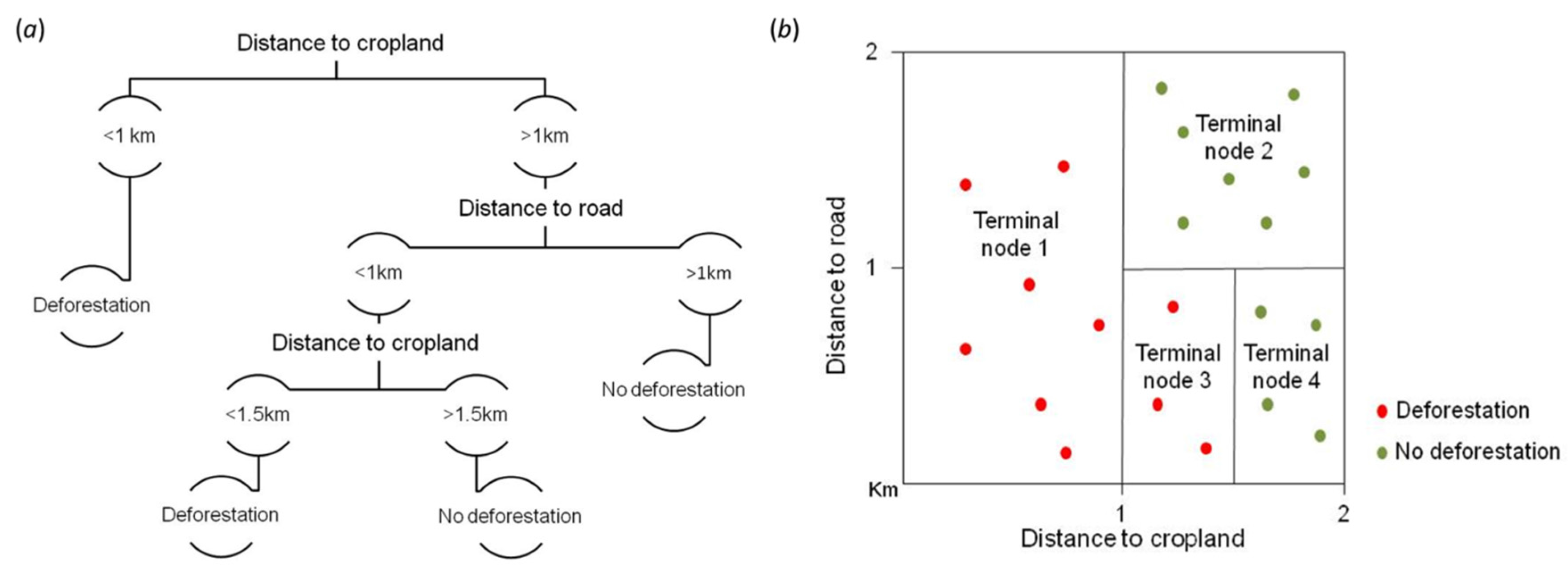
2.1. Random Forests
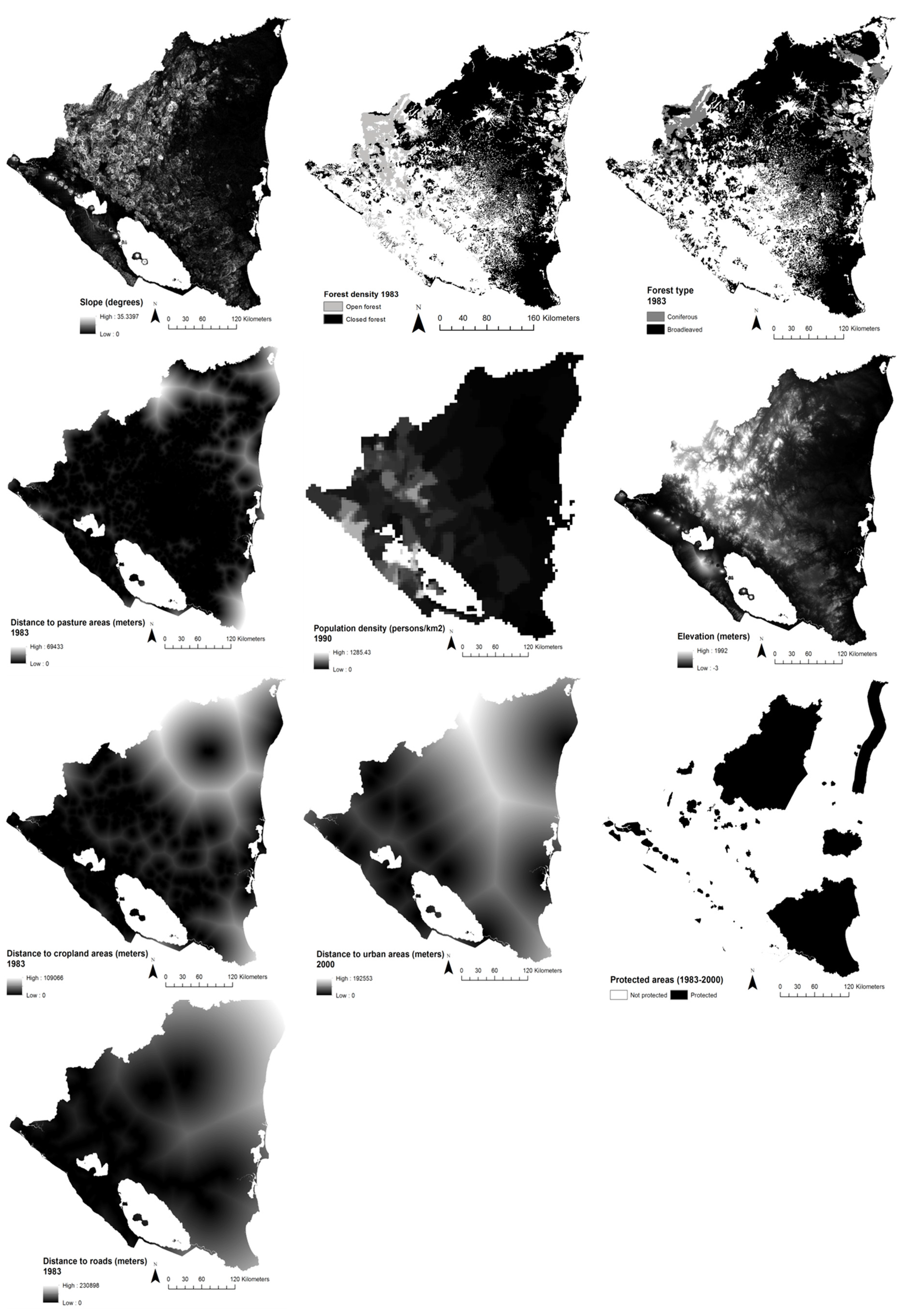
2.2. Data Used and Variable Selection
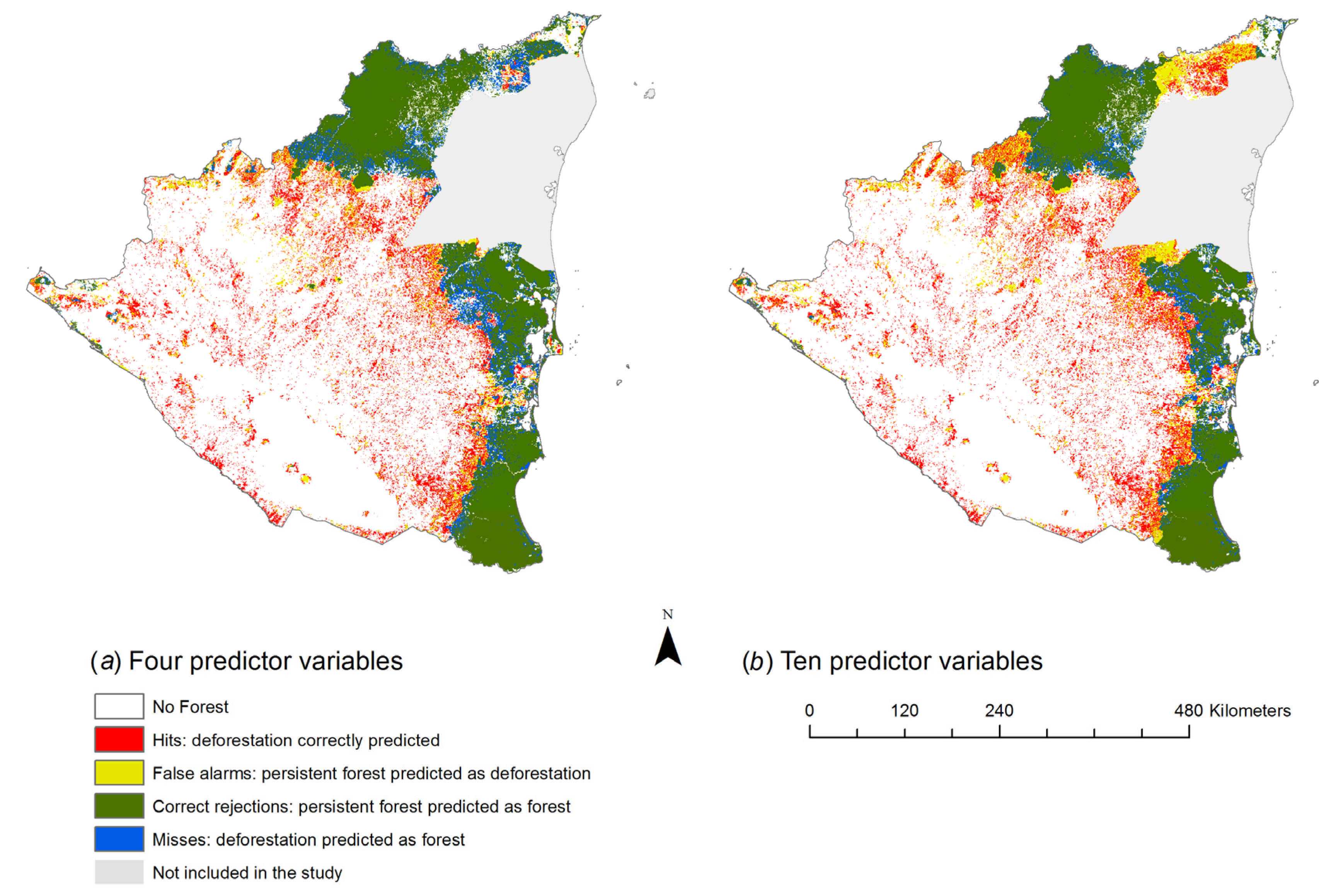
2.3. Modeling Using 10 and Four Predictors
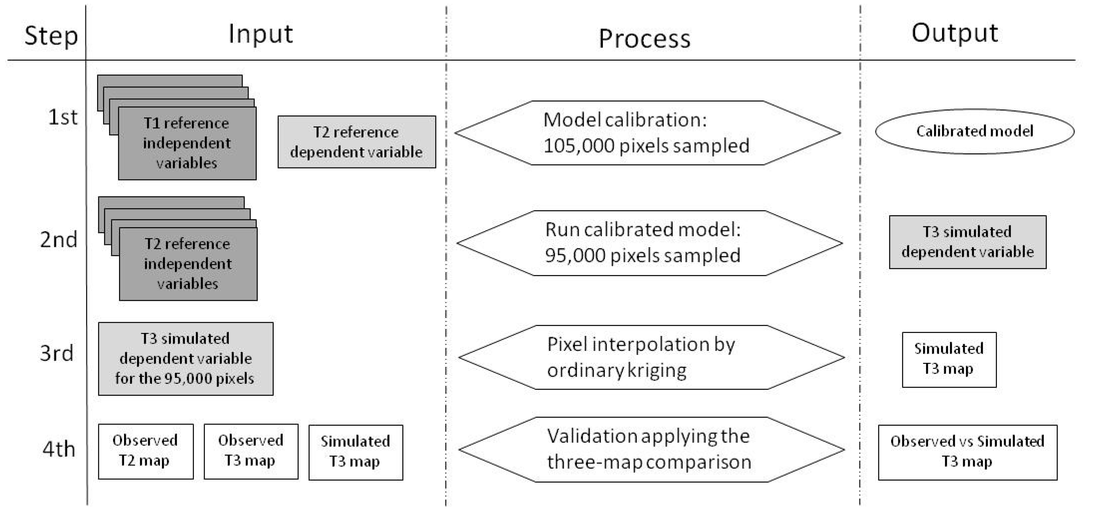
2.4. Model Calibration
2.5. Model Validation
- Approximately 95,000 sample pixels were generated by adopting a random sampling from the class “forest” at time t2.
- For each pixel randomly selected, the corresponding value from every map of the independent variables at t2 was extracted.
- The calibrated model and the fitted parameters used in the calibration procedure were used to predict the dependent variable at time t3 for the 95,000 pixels.
- The t3-simulated map, which displays the predicted risk of deforestation, was created by interpolating the entire set of pixels using kriging.
- The performance of the model was assessed by applying the three-map comparison technique and other statistical indicators [46].
2.6. Study Area
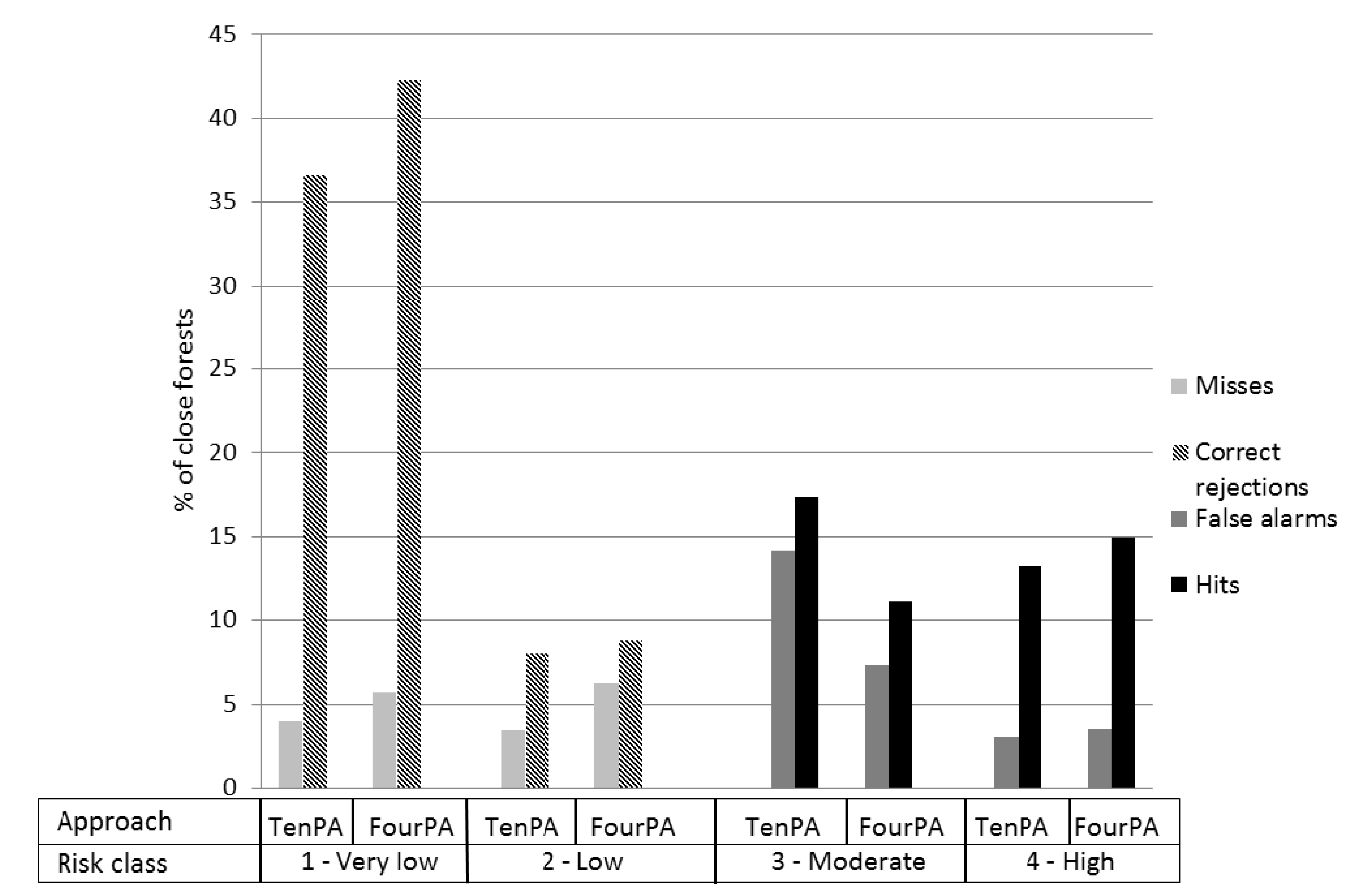
3. Results
4. Discussion
5. Conclusions
Acknowledgments
Author Contributions
Conflicts of Interest
References
- Intergovernmental Panel on Climate Change. Summary for Policymakers. In Climate Change 2013: The Physical Science Basis; Contribution of Working Group I to the Fifth Assessment Report of the IPCC; Stocker, T.F., Qin, D., Plattner, G.-K., Tignor, M., Allen, S.K., Boschung, J., Nauels, A., Xia, Y., Bex, V., Midgley, P.M., Eds.; Cambridge University Press: Cambridge, UK; New York, NY, USA, 2013. [Google Scholar]
- Bonan, G.B. Forests and Climate Change: Forcings, Feedbacks, and the Climate Benefits of Forests. Science 2008, 320, 1444–1449. [Google Scholar] [CrossRef] [PubMed]
- Van der Werf, G.R.; Morton, D.C.; DeFries, R.S.; Olivier, J.G.; Kasibhatla, P.S.; Jackson, R.B.; Collatz, G.J.; Randerson, J.T. CO2 emissions from forest loss. Nat. Geosci. 2009, 2, 737–738. [Google Scholar] [CrossRef]
- Intergovernmental Panel on Climate Change. Carbon and Other Biogeochemical Cycles. In Climate Change 2013: The Physical Science Basis; Contribution of Working Group I to the Fifth Assessment Report of the IPCC; Stocker, T.F., Qin, D., Plattner, G.-K., Tignor, M., Allen, S.K., Boschung, J., Nauels, A., Xia, Y., Bex, V., Midgley, P.M., Eds.; Cambridge University Press: Cambridge, UK; New York, NY, USA, 2013. [Google Scholar]
- United Nations Framework Convention on Climate Change. Report of the Conference of the Parties on Its Sixteenth Session, Held in Cancun from 29 November to 10 December 2010 Addendum Part Two: Action Taken by the Conference of the Parties 2007 at Its Thirteenth Session; Distributed 15 March 2011; United Nations Office at Geneva: Geneva, Switzerland, 2011. [Google Scholar]
- Streck, C. Financing REDD+: Matching needs and ends. Curr. Opin. Environ. Sustain. 2012, 4, 628–637. [Google Scholar] [CrossRef]
- Lin, L.; Sills, E.; Cheshire, H. Targeting areas for Reducing Emissions from Deforestation and Forest Degradation (REDD+) Projects in Tanzania. Glob. Environ. Chang. 2014, 24, 277–286. [Google Scholar] [CrossRef]
- Wendland, K.J.; Honzák, M.; Portela, R.; Vitale, B.; Rubinoff, S.; Randrianarisoa, J. Targeting and implementing payments for ecosystem services: Opportunities for bundling biodiversity conservation with carbon and water services in Madagascar. Ecol. Econ. 2010, 69, 2093–2107. [Google Scholar] [CrossRef]
- Kim, O.S. An Assessment of Deforestation Models for Reducing Emissions from Deforestation and Forest Degradation (REDD): An Assessment of Deforestation Models for REDD. Trans. GIS 2010, 14, 631–654. [Google Scholar] [CrossRef]
- Köhl, M.; Baldauf, T.; Plugge, D.; Krug, J. Reduced emissions from deforestation and forest degradation (REDD): A climate change mitigation strategy on a critical track. Carbon Balance Manag. 2009, 4, 10. [Google Scholar] [CrossRef] [PubMed]
- Harris, N.L.; Petrova, S.; Stolle, F.; Brown, S. Identifying optimal areas for REDD intervention: East Kalimantan, Indonesia as a case study. Environ. Res. Lett. 2008, 3, 035006. [Google Scholar] [CrossRef]
- Plugge, D.; Baldauf, T.; Köhl, M. The global climate change mitigation strategy REDD: Monitoring costs and uncertainties jeopardize economic benefits. Clim. Chang. 2013, 119, 247–259. [Google Scholar] [CrossRef]
- Romijn, E.; Lantican, C.B.; Herold, M.; Lindquist, E.; Ochieng, R.; Wijaya, A.; Murdiyarso, D.; Verchot, L. Assessing change in national forest monitoring capacities of 99 tropical countries. For. Ecol. Manag. 2015, 352, 109–123. [Google Scholar] [CrossRef]
- Boyd, D.S. A review of “Modelling Deforestation Processes:” A review. Trees Series B Report n° l. By E.F. Lambin. Int. J. Remote Sens. 1996, 17, 1061–1062. [Google Scholar] [CrossRef]
- Dudley, R.G. A little REDD model to quickly compare possible baseline and policy scenarios for reducing emissions from deforestation and forest degradation. Mitig. Adapt. Strateg. Glob. Chang. 2010, 15, 53–69. [Google Scholar] [CrossRef]
- Gutierrez-Velez, V.H.; Pontius, R.G. Influence of carbon mapping and land change modelling on the prediction of carbon emissions from deforestation. Environ. Conserv. 2012, 39, 325–336. [Google Scholar] [CrossRef]
- Jong, B.H.J.; Hellier, A.; Castillo-Santiago, M.A.; Tipper, R. Application of the “Climafor” Approach to Estimate Baseline Carbon Emissions of a Forest Conservation Project in the Selva Lacandona, Chiapas, Mexico. Mitig. Adapt. Strateg. Glob. Chang. 2005, 10, 265–278. [Google Scholar] [CrossRef]
- Veldkamp, A.; Fresco, L.O. CLUE-CR: An integrated multi-scale model to simulate land use change scenarios in Costa Rica. Ecol. Model. 1996, 91, 231–248. [Google Scholar] [CrossRef]
- Kamusoko, C.; Oono, K.; Nakazawa, A.; Wada, Y.; Nakada, R.; Hosokawa, T.; Tomimura, S.; Furuya, T.; Iwata, A.; Moriike, H.; et al. Spatial Simulation Modelling of Future Forest Cover Change Scenarios in Luangprabang Province, Lao PDR. Forests 2011, 2, 707–729. [Google Scholar] [CrossRef]
- Aguilar-Amuchastegui, N.; Forrest, J.L. A Review of Tools and Approaches to Compare Business-as-Usual to REDD+ Scenarios. Available online: http://wwf.panda.org/?209271/REDD-MRV-tools (accessed on 20 January 2017).
- Aguilar-Amuchastegui, N.; Riveros, J.C.; Forrest, J.L. Identifying areas of deforestation risk for REDD+ using a species modeling tool. Carbon Balance Manag. 2014, 9, 10. [Google Scholar] [CrossRef] [PubMed]
- Huettner, M.; Leemans, R.; Kok, K.; Ebeling, J. A comparison of baseline methodologies for “Reducing Emissions from Deforestation and Degradation”. Carbon Balance Manag. 2009, 4, 4. [Google Scholar] [CrossRef] [PubMed]
- Breiman, L. Random forests. Mach. Learn. 2001, 45, 5–32. [Google Scholar] [CrossRef]
- James, G.; Witten, D.; Hastie, T.; Tibshirani, R. An Introduction to Statistical Learning; Springer Texts in Statistics; Springer: New York, NY, USA, 2013; Volume 103. [Google Scholar]
- Kuhn, M.; Johnson, K. Applied Predictive Modeling; Springer: New York, NY, USA, 2013. [Google Scholar]
- Prasad, A.M.; Iverson, L.R.; Liaw, A. Newer Classification and Regression Tree Techniques: Bagging and Random Forests for Ecological Prediction. Ecosystems 2006, 9, 181–199. [Google Scholar] [CrossRef]
- Ministerio Agropecuario y Forestal. Cobertura Forestal, Shapefile, Scale 1:250000; Ministerio Agropecuario y Forestal: Managua, Nicaragua, 1983. [Google Scholar]
- Ministerio Agropecuario y Forestal. Cobertura Forestal, Shapefile, Scale 1:250000; Ministerio Agropecuario y Forestal: Managua, Nicaragua, 2000. [Google Scholar]
- Ministerio Agropecuario y Forestal. Valoración Forestal Nicaragua, 2000, 1st ed.; Ministerio Agropecuario y Forestal: Managua, Nicaragua, 2005. [Google Scholar]
- Ministerio del Ambiente y Recursos Naturales-Ministerio Agropecuario y Forestal. Mapa de Uso Actual, Shapefile, Scale 1:250000; Ministerio del Ambiente y Recursos Naturales-Ministerio Agropecuario y Forestal: Managua, Nicaragua, 2011. [Google Scholar]
- Lehner, B.; Verdin, K.; Jarvi, A. HydroSHEDS Technical Documentation; World Wildlife Fund US: Washington, DC, USA, 2006. [Google Scholar]
- Center for International Earth Science Information Network; Columbia University; Centro Internacional de Agricultura Tropical. Gridded Population of the World, Version 3 (GPWv3): Population Density Grid; NASA Socioeconomic Data and Applications Center (SEDAC): Palisades, NY, USA, 2005. [Google Scholar]
- International Union for Conservation of Nature and Natural Resources; United Nations Environment Programme World Conservation Monitoring Centre; United Nations Environment Programme. The World Database on Protected Areas; World Conservation Monitoring Centre: Cambridge, UK, 2014. [Google Scholar]
- Instituto Nacional de Estudios Territoriales. Red Nacional de Caminos (Shapefile); Instituto Nacional de Estudios Territoriales: Managua, Nicaragua, 1983. [Google Scholar]
- Instituto Nacional de Estudios Territoriales. Red Nacional de Caminos (Shapefile); Instituto Nacional de Estudios Territoriales: Managua, Nicaragua, 2000. [Google Scholar]
- Instituto Nacional de Estudios Territoriales. Ciudades y Comarcas (Shapefile); Instituto Nacional de Estudios Territoriales: Managua, Nicaragua, 2000. [Google Scholar]
- Food and Agricultural Organization. Global Forest Resources Assessment 2000; Food and Agricultural Organization: Rome, Italy, 2000. [Google Scholar]
- United Nations Framework Convention on Climate Change. Report of the Conference of the Parties serving as the meeting of the Parties to the Kyoto Protocol on its first session, held at Montreal from 28 November to 10 December 2005 Addendum. Part Two: Action taken by the Conference of the Parties serving as the meeting of the Parties to the Kyoto Protocol at its first session. Available online: http://unfccc.int/resource/docs/2005/cmp1/eng/08a04.pdf (accessed on 20 January 2017).
- Hosonuma, N.; Herold, M.; De Sy, V.; De Fries, R.S.; Brockhaus, M.; Verchot, L.; Angelsen, A.; Romijn, E. An assessment of deforestation and forest degradation drivers in developing countries. Environ. Res. Lett. 2012, 7, 44009. [Google Scholar] [CrossRef]
- Instituto Nacional Forestal. Resultados del Inventario Nacional Forestal: Nicaragua 2007–2008; Instituto Nacional Forestal: Managua, Nicaragua, 2009. [Google Scholar]
- Zeledon, E.B.; Kelly, N.M. Understanding large-scale deforestation in southern Jinotega, Nicaragua from 1978 to 1999 through the examination of changes in land use and land cover. J. Environ. Manag. 2009, 90, 2866–2872. [Google Scholar] [CrossRef] [PubMed]
- Gourdji, S.; Läderach, P.; Valle, A.M.; Martinez, C.Z.; Lobell, D.B. Historical climate trends, deforestation, and maize and bean yields in Nicaragua. Agric. For. Meteorol. 2015, 200, 270–281. [Google Scholar] [CrossRef]
- Ministerio del Ambiente y Recursos Naturales. Readiness Preparation Proposal, Formal Version 7; Ministerio del Ambiente y Recursos Naturales: Managua, Nicaragua, 2013. [Google Scholar]
- Redo, D.J.; Grau, H.R.; Aide, T.M.; Clark, M.L. Asymmetric forest transition driven by the interaction of socioeconomic development and environmental heterogeneity in Central America. Proc. Natl. Acad. Sci. USA 2012, 109, 8839–8844. [Google Scholar] [CrossRef] [PubMed]
- R Core Team. R: A Language and Environment for Statistical Computing; R Foundation for Statistical Computing: Vienna, Austria, 2015. [Google Scholar]
- Pontius, R.G.; Boersma, W.; Castella, J.-C.; Clarke, K.; de Nijs, T.; Dietzel, C.; Duan, Z.; Fotsing, E.; Goldstein, N.; Kok, K.; et al. Comparing the input, output, and validation maps for several models of land change. Ann. Reg. Sci. 2008, 42, 11–37. [Google Scholar] [CrossRef]
- Webster, R.; Oliver, M.A. Geostatistics for Environmental Scientists (Statistics in Practice), 2nd ed.; Wiley: Chichester, UK, 2007. [Google Scholar]
- Pontius, R.G.; Millones, M. Death to Kappa: Birth of quantity disagreement and allocation disagreement for accuracy assessment. Int. J. Remote Sens. 2011, 32, 4407–4429. [Google Scholar] [CrossRef]
- Committee on Needs and Research Requirements for Land Change Modeling; Geographical Sciences Committee; Board on Earth Sciences and Resources; Division on Earth and Life Studies; National Research Council. Advancing Land Change Modeling: Opportunities and Research Requirements; National Academies Press: Washington, DC, USA, 2014. [Google Scholar]
- Ministerio del Ambiente y Recursos Naturales; International Union for Conservation of Nature and Natural Resources. Estado de la Gestion Compartida de Areas Protegidas en Nicaragua, 1st ed.; IUCN Mesoamérica: San José, Costa Rica, 2005. [Google Scholar]
- Food and Agricultural Organization. Global Forest Resources Assessment; Food and Agricultural Organization: Rome, Italy, 2015. [Google Scholar]
- Maldidier, C. Tendencias Actuales de la Frontera Agrícola en Nicaragua; Nitlapan-UCA: Managua, Nicaragua, 1993. [Google Scholar]
- Pacheco, P.; Aguilar-Støen, M.; Börner, J.; Etter, A.; Putzel, L.; Diaz, M.D.C.V. Landscape Transformation in Tropical Latin America: Assessing Trends and Policy Implications for REDD+. Forests 2010, 2, 1–29. [Google Scholar] [CrossRef]
- Cutler, D.R.; Edwards, T.C., Jr.; Beard, K.H.; Cutler, A.; Hess, K.T.; Gibson, J.; Lawler, J.J. Random forests for classification in ecology. Ecology 2007, 88, 2783–2792. [Google Scholar] [CrossRef] [PubMed]
- Griffith, D.A.; Peres-Neto, P.R. Spatial modeling in ecology: The flexibility of eigenfunction spatial analyses. Ecology 2006, 87, 2603–2613. [Google Scholar] [CrossRef]
- Pirard, R.; Karsenty, A. Climate Change Mitigation: Should “Avoided Deforestation” Be Rewarded? J. Sustain. For. 2009, 28, 434–455. [Google Scholar] [CrossRef]
- Sloan, S.; Pelletier, J. How accurately may we project tropical forest-cover change? A validation of a forward-looking baseline for REDD. Glob. Environ. Chang. 2012, 22, 440–453. [Google Scholar] [CrossRef]
- Angelsen, A.; Rudel, T.K. Designing and Implementing Effective REDD + Policies: A Forest Transition Approach. Rev. Environ. Econ. Policy 2013, 7, 91–113. [Google Scholar] [CrossRef]
- Patel, T.; Dhiaulhaq, A.; Gritten, D.; Yasmi, Y.; De Bruyn, T.; Paudel, N.; Luintel, H.; Khatri, D.; Silori, C.; Suzuki, R. Predicting Future Conflict under REDD+ Implementation. Forests 2013, 4, 343–363. [Google Scholar] [CrossRef]
- Angelsen, A.; Ainembabazi, J.H.; Bauch, S.C.; Herold, M.; Verchot, L.; Hänsel, G.; Schueler, V.; Toop, G.; Gilbert, A.; Eisbrenner, K. Testing Methodologies for REDD+: Deforestation Drivers, Costs and Reference Levels; ECOFYS: London, UK, 2013. [Google Scholar]
- United Nations Framework Convention on Climate Change. Report of the Conference of the Parties on its seventeenth session, held in Durban from 28 November to 11 December 2011 Addendum Part Two: Action taken by the Conference of the Parties at its seventeenth session. Available online: http://unfccc.int/resource/docs/2011/cop17/eng/09a01.pdf (accessed on 20 January 2017).
- Herold, M.; Angelsen, A.; Verchot, L.V.; Wijaya, A.; Ainembabazi, J.H. A stepwise framework for developing REDD+ reference levels. In Analysing REDD+: Challenges and Choices; Angelsen, A., Brockhaus, M., Sunderlin, W.D., Verchot, L.V., Eds.; Center for International Forestry Research: Bogor, Indonesia, 2012; pp. 279–299. [Google Scholar]


| Source Map | Data Format | Years Covered | Variable Extracted | Reference Unit | Sources |
|---|---|---|---|---|---|
| Land cover | Vector | 1983 | - Distance to pasture areas | Meters | [27] |
| - Distance to cropland areas | Meters | ||||
| - Forest type | Broadleaved/coniferous | ||||
| - Forest density | Closed forest/open forest | ||||
| Land cover | Vector | 2000 | - Distance to pasture areas | Meters | [28] |
| - Distance to cropland areas | Meters | ||||
| - Forest type | Broadleaved/coniferous | ||||
| - Forest density | Closed forest/open forest | ||||
| - Forest cover change | Forest/deforestation | ||||
| Land cover | Vector | 2011 | - Forest cover change | Forest/deforestation | [30] |
| Digital Elevation Model | Raster | - | - Altitude | Meters above sea level | [31] |
| Gridded Population of the World | Raster | 1990, 2000 | - Population density | Persons/km2 | [32] |
| - Slope | Degrees | ||||
| Protected areas | Raster | From 1980 to 2000 | - Presence/absence of protected areas | Protected/No protected | [33] |
| Road network | Vector | 1983, 2000 | - Distance to road | Meters | [34,35] |
| Urban settlement | Vector | - | - Distance to urban areas | Meters | [36] |
| Screened Predictor Variables | |
|---|---|
| Used in TenPA | Used in FourPA |
| Forest density | Altitude |
| Population density | Distance to cropland areas |
| Distance to cropland areas | Slope |
| Protected areas | Distance to pasture areas |
| Forest type | |
| Altitude | |
| Distance to roads | |
| Distance to urban areas | |
| Slope | |
| Distance to pasture areas | |
| Reference | ||||||
|---|---|---|---|---|---|---|
| TenPA | FourPA | |||||
| Forest | Deforestation | Simulated Total | Forest | Deforestation | Simulated Total | |
| Forest | 44.7 | 7.5 | 52.2 | 51.2 | 12 | 63.2 |
| Deforestation | 17.3 | 30.5 | 47.8 | 10.8 | 26 | 36.8 |
| Reference Total | 62 | 38 | 100 | 62 | 38 | 100 |
| Ten Predictors (TenPA) | Four Predictors (FourPA) | |
|---|---|---|
| Overall accuracy | 76% | 76% |
| Producer’s accuracy | 0.80 | 0.69 |
| User’s accuracy | 0.64 | 0.71 |
| Figure of merit | 55% | 53% |
© 2017 by the authors; licensee MDPI, Basel, Switzerland. This article is an open access article distributed under the terms and conditions of the Creative Commons Attribution (CC BY) license (http://creativecommons.org/licenses/by/4.0/).
Share and Cite
Di Lallo, G.; Mundhenk, P.; Zamora López, S.E.; Marchetti, M.; Köhl, M. REDD+: Quick Assessment of Deforestation Risk Based on Available Data. Forests 2017, 8, 29. https://doi.org/10.3390/f8010029
Di Lallo G, Mundhenk P, Zamora López SE, Marchetti M, Köhl M. REDD+: Quick Assessment of Deforestation Risk Based on Available Data. Forests. 2017; 8(1):29. https://doi.org/10.3390/f8010029
Chicago/Turabian StyleDi Lallo, Giulio, Philip Mundhenk, Sheila Edith Zamora López, Marco Marchetti, and Michael Köhl. 2017. "REDD+: Quick Assessment of Deforestation Risk Based on Available Data" Forests 8, no. 1: 29. https://doi.org/10.3390/f8010029