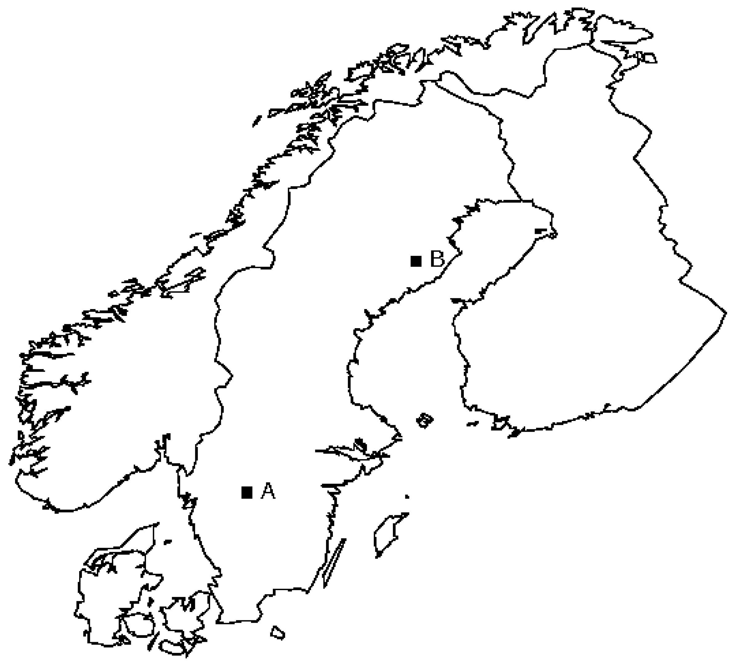
Figure 1.
Location of the test sites in Sweden. A: Remningstorp test site; B: Svartberget test site.
Figure 1.
Location of the test sites in Sweden. A: Remningstorp test site; B: Svartberget test site.
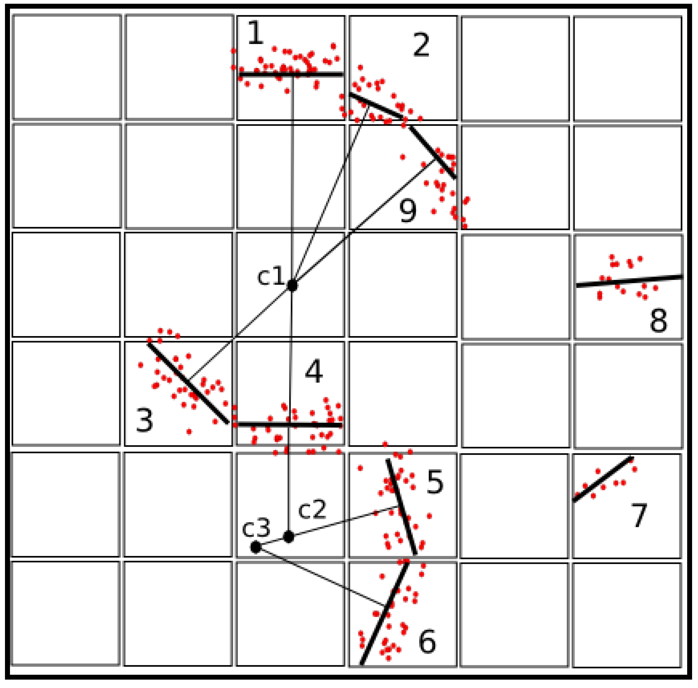
Figure 2.
Two-dimensional view of the three-dimensional grid. Cells 1–9 contain laser data points. In each grid cell, a plane (thick line) is derived from the laser data points using the eigenvectors and eigenvalues. The centers c1–c3 are derived from the normals (thin lines) of two connected planes. The plane in Cell 4 is connected to two centers. Planes with several possible centers are connected to the center with the highest weight. The planes in Cells 7 and 8 are not connected to any neighbor and, therefore, not connected to possible tree stem centers.
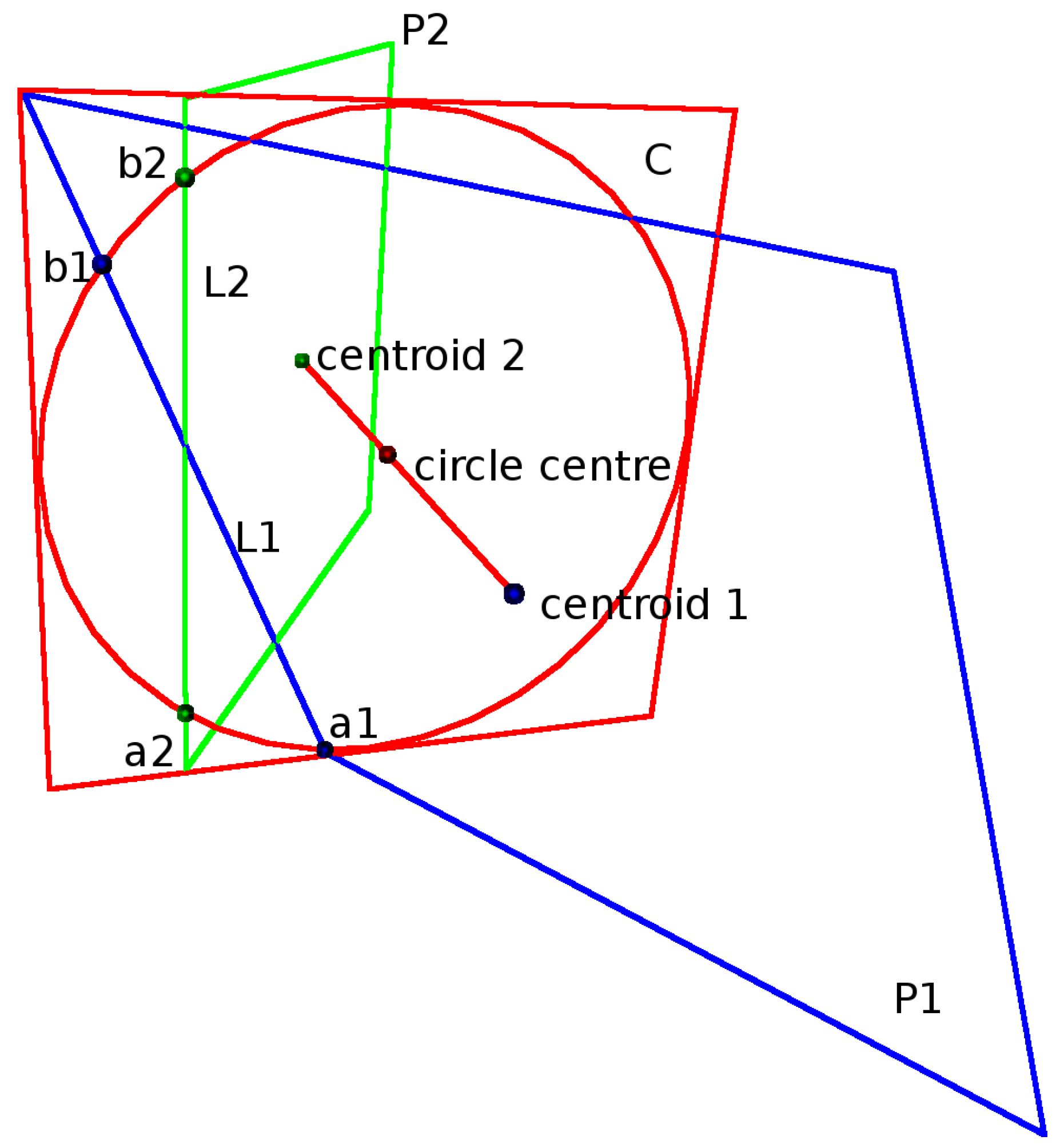
Figure 3.
Plane P1 and plane P2 are derived from point clouds with Centroid 1 and Centroid 2. An intersecting plane C with a circle is positioned in between the two point cloud centroids. L1 is the intersecting line between plane P1 and plane C. L2 is the intersecting line between plane P2 and plane C. a1 and b1 are the intersecting points between the circle and L1. a2 and b2 are the intersecting points between the circle and L2. A measure of how well the two planes connect is evaluated by measuring the distances from points a1,b1 and a2, b2 to the opposite intersecting line.
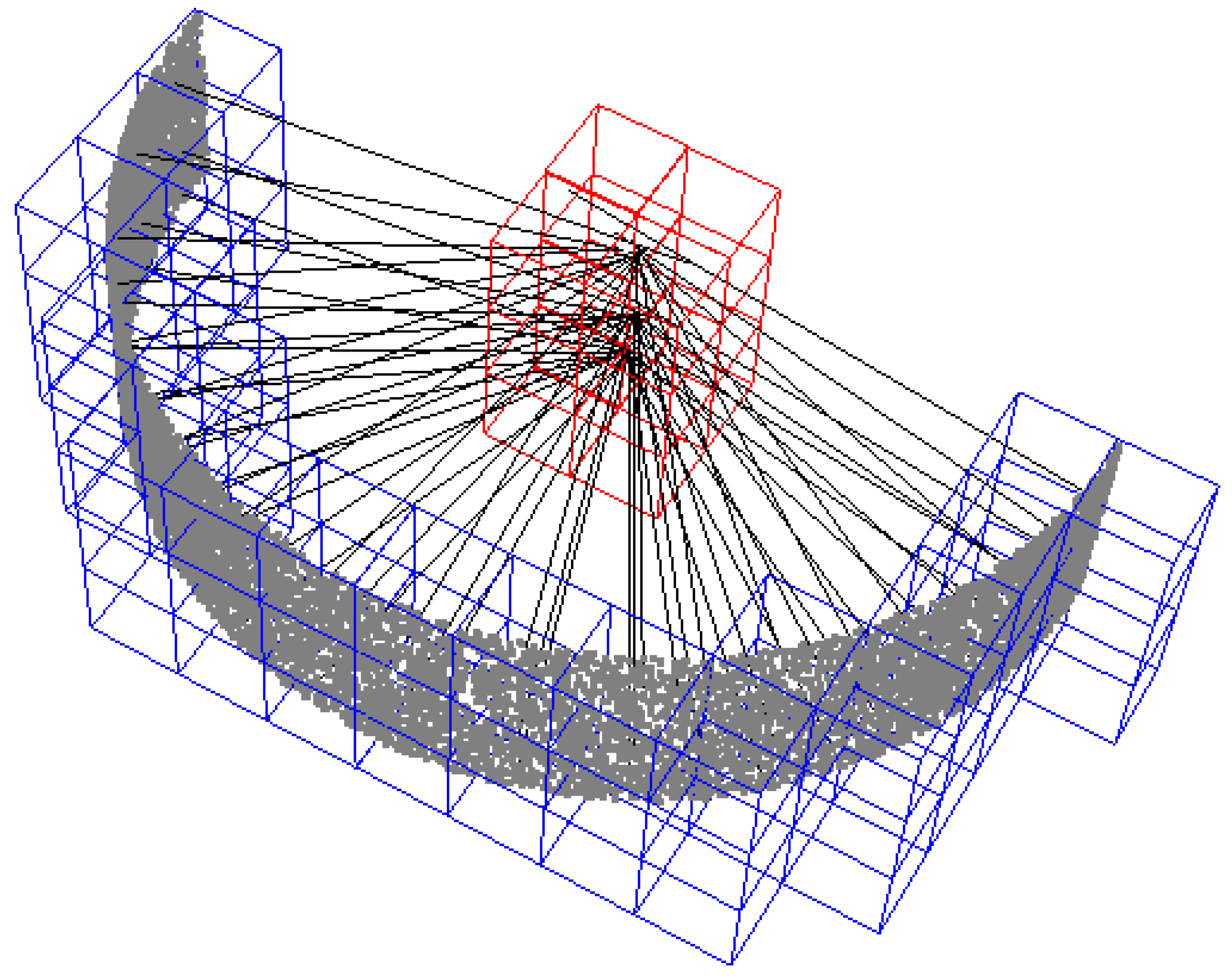
Figure 4.
Synthetic data points of a semi-cylinder of height 7 cm and radius 15 cm. The blue voxels, containing cylinder surface points, are connected to the cylinder center voxels in red. All cylinder surface points that are connected to the cylinder center cluster in red are used in the estimate of the stem diameter. The data points in this example are filtered with a cluster weight of 15 and a curve weight of 0.75. The grid cell size is 3 × 3 × 3 cm3.
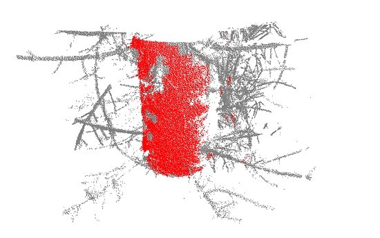
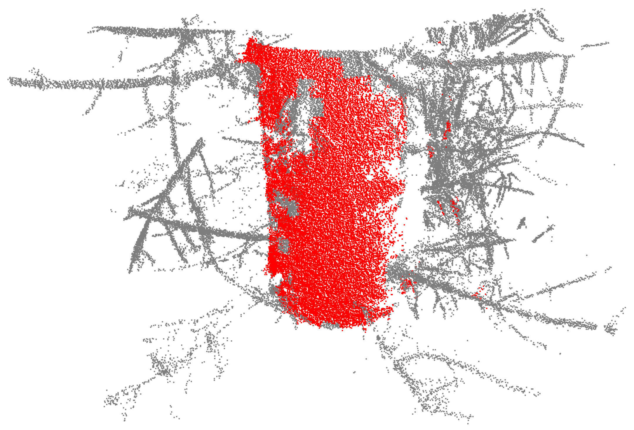
Figure 5.
Lidar data points of a tree with a diameter at breast height of 26.35 cm cut out from 1.05–1.55 m above the ground. The data points in this example are filtered with a cluster weight of 15 and a curve weight of 0.75. The grid cell size is 3 × 3 × 3 cm3. The red data points have values above the threshold and are used when cylinder fitting the data.
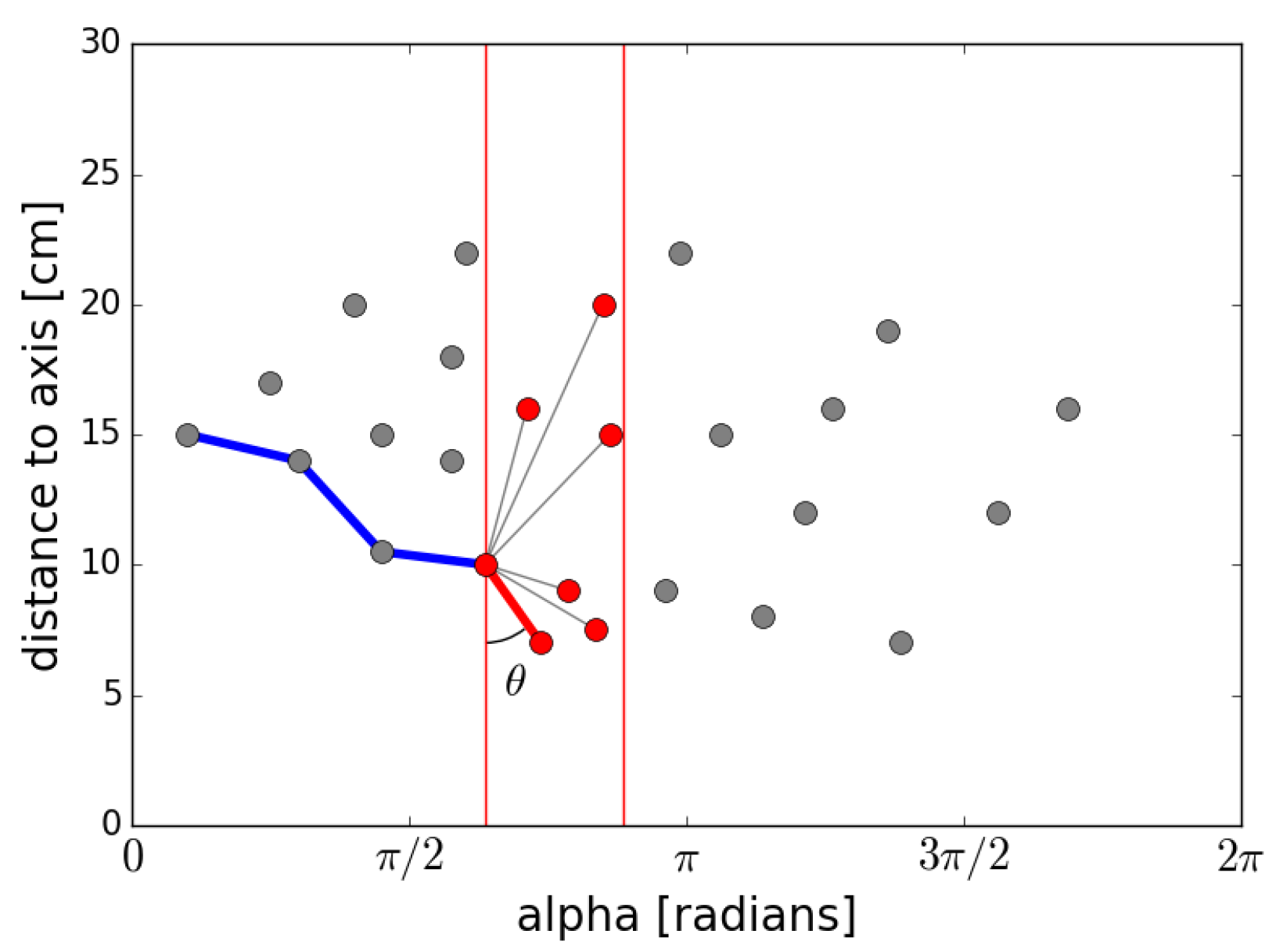
Figure 6.
Illustration of the moving window convex hull algorithm designed to find the innermost part of the point dataset. The blue lines are found in earlier iteration steps. The red points are within the current search window. The point that gives the smallest angle θ measured from the y-axis is chosen as the next starting point. The thick red line is the line that is chosen by the algorithm. The thin grey lines are discarded. The search window is then moved to the new starting point for the following iteration steps.
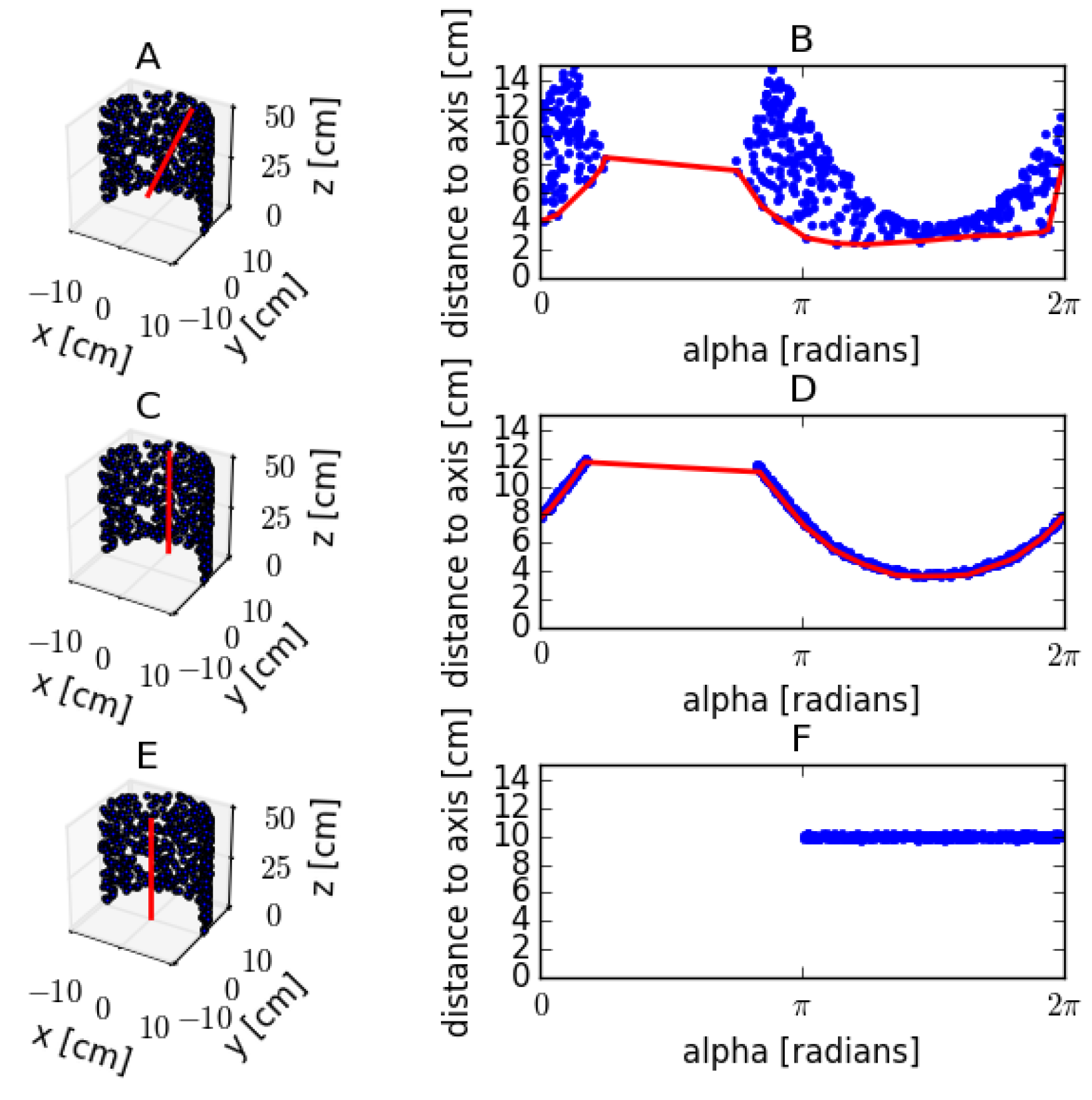
Figure 7.
Cylinder fitting of a synthetic point dataset with radius 0.10 m. (A,C,E) The perspective views of semi-cylinder point data with different axis positions. The axis positions are marked in red. (A) The axis is positioned at the centroid of the point dataset and tilted 10°; (C) the axis is positioned at the centroid of the point dataset and is aligned with the true cylinder axis; (E) the axis is positioned at the true center of the cylinder and is aligned with the true cylinder axis. (B,D,F) The radial displacement as a function of the angle of the axis positions in (A,C,E); the red lines in (B,D) are calculated by a moving window convex hull algorithm and are used as a base level from which to calculate the deviation of the dataset.
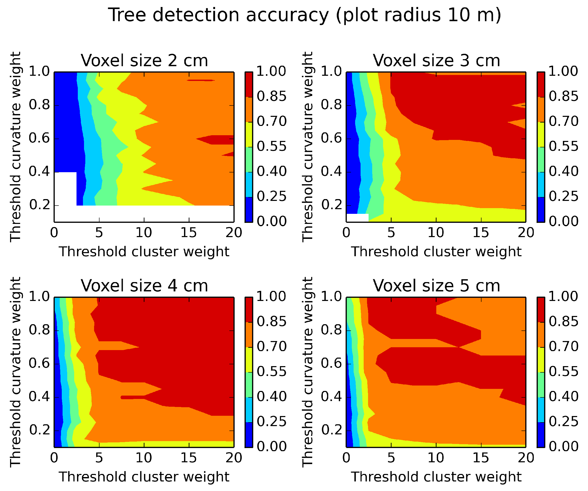
Figure 8.
Tree detection accuracy evaluated on a plot of a radius of 10 m and different parameter settings. White areas indicate missing data. High threshold parameter settings give high tree detection accuracy, with the exception of a voxel size of 5 cm, which is optimal with medium threshold parameter settings.
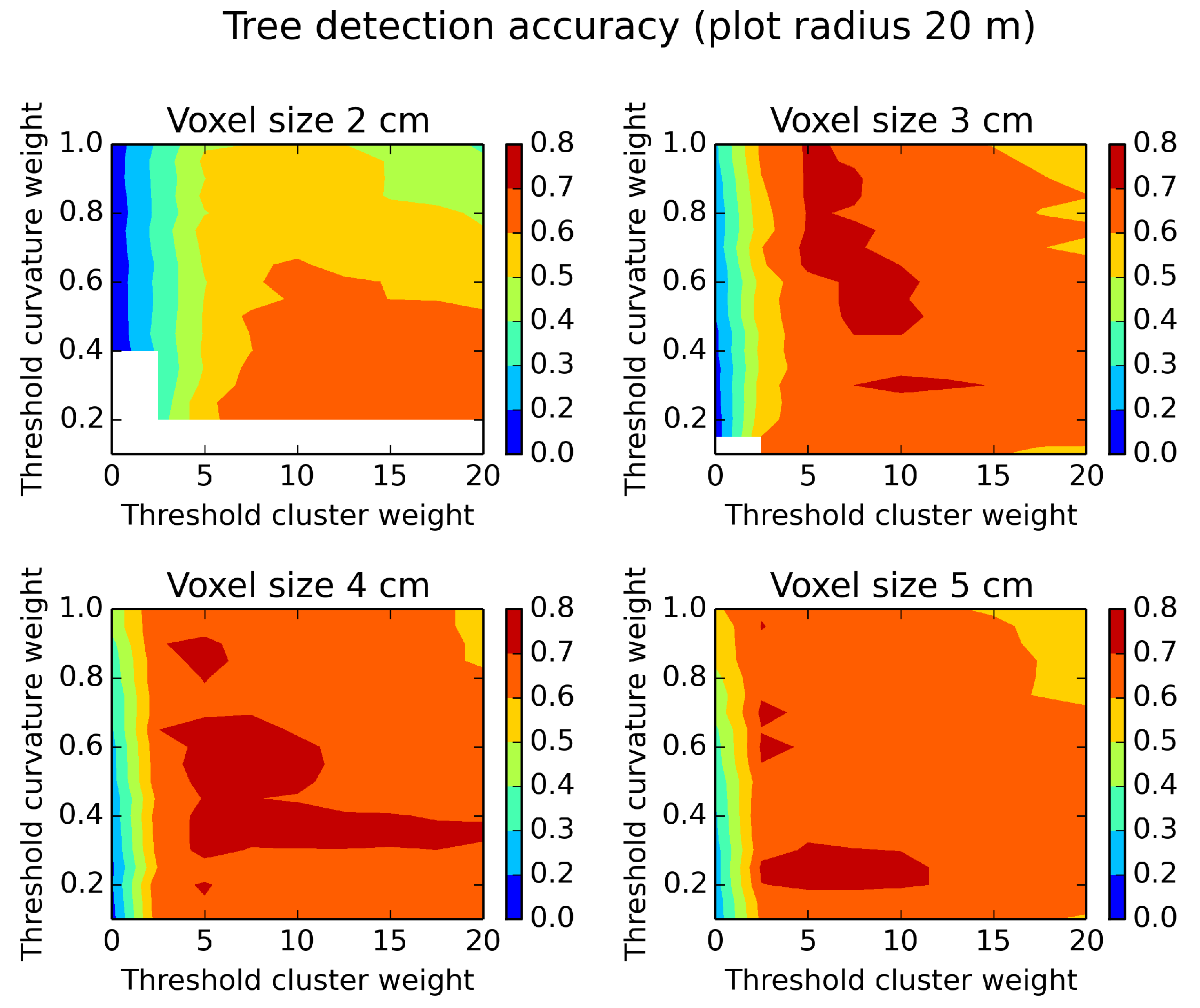
Figure 9.
Tree detection accuracy evaluated on a plot of a radius of 20 m and different parameter settings. White areas indicate missing data. The optimum for high tree detection accuracy is achieved with different parameter settings for different voxel sizes.
Figure 9.
Tree detection accuracy evaluated on a plot of a radius of 20 m and different parameter settings. White areas indicate missing data. The optimum for high tree detection accuracy is achieved with different parameter settings for different voxel sizes.
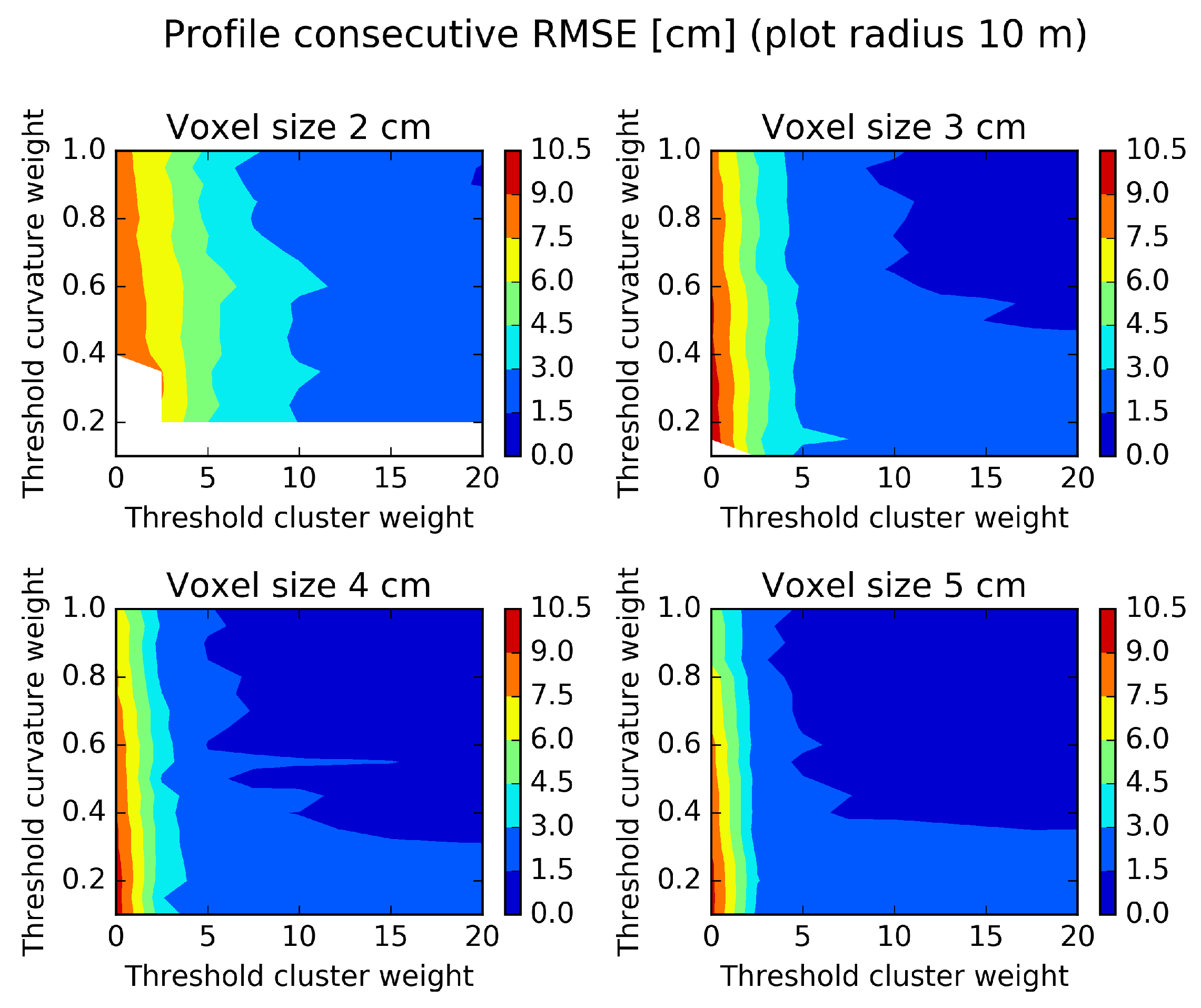
Figure 10.
Profile consecutive diameter RMSE evaluated on a plot of a radius of 10 m and different parameter settings. White areas indicate missing data. High parameter threshold values give smooth stem profiles.
Figure 10.
Profile consecutive diameter RMSE evaluated on a plot of a radius of 10 m and different parameter settings. White areas indicate missing data. High parameter threshold values give smooth stem profiles.
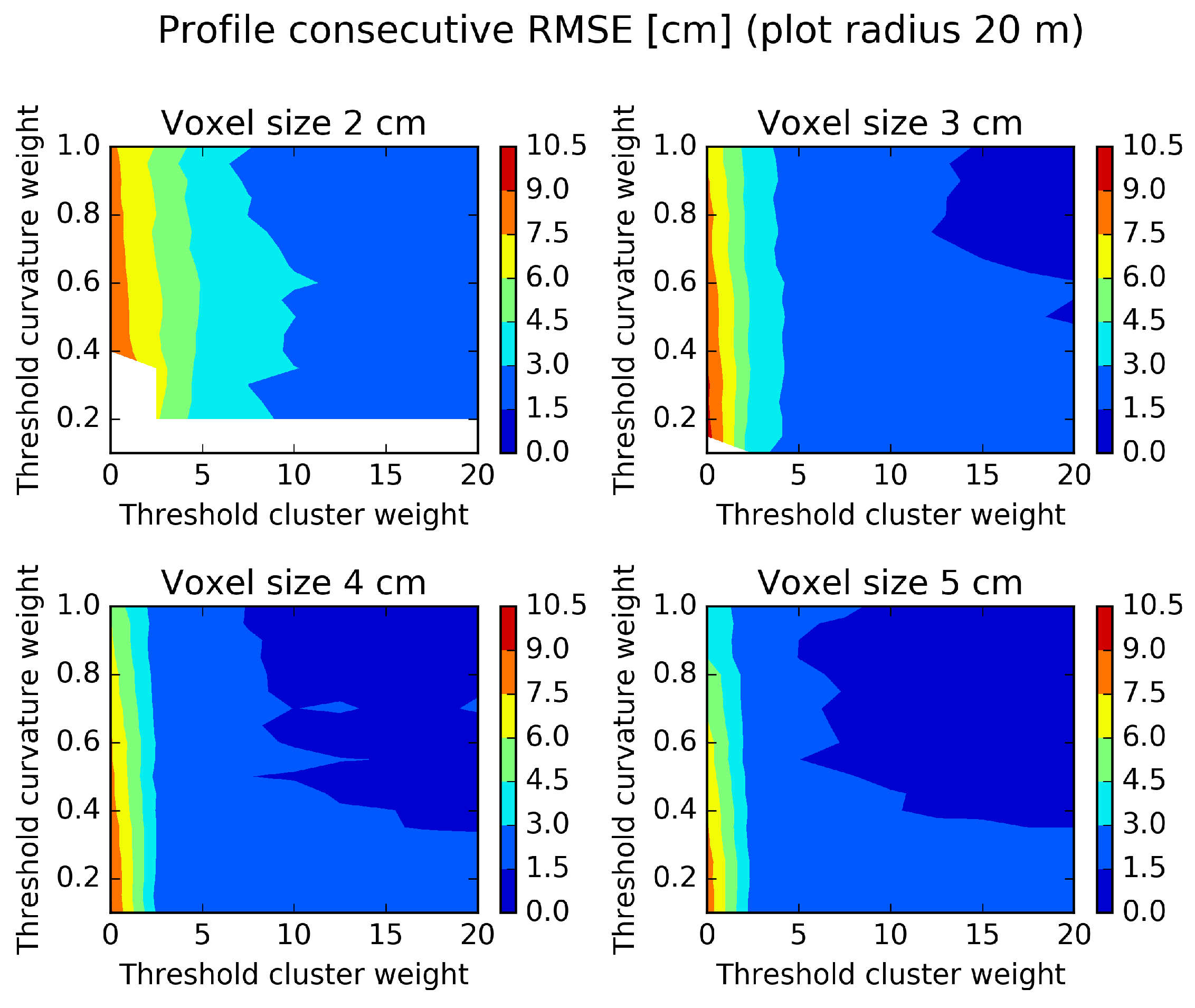
Figure 11.
Profile consecutive diameter RMSE evaluated on a plot of a radius of 20 m and different parameter settings. White areas indicate missing data. High parameter threshold values give smooth stem profiles.
Figure 11.
Profile consecutive diameter RMSE evaluated on a plot of a radius of 20 m and different parameter settings. White areas indicate missing data. High parameter threshold values give smooth stem profiles.
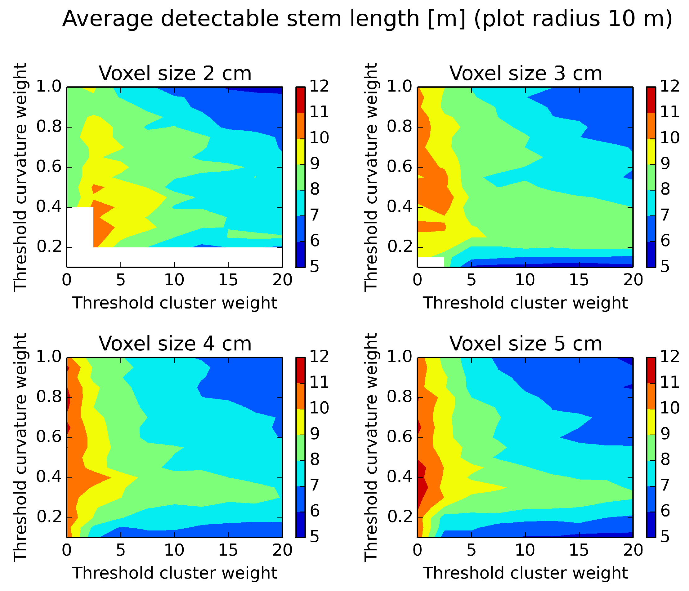
Figure 12.
Average detectable stem length evaluated on a plot of a radius of 10 m and different parameter settings. White areas indicate missing data. Low threshold parameter values give many estimated stem diameters along the tree.
Figure 12.
Average detectable stem length evaluated on a plot of a radius of 10 m and different parameter settings. White areas indicate missing data. Low threshold parameter values give many estimated stem diameters along the tree.
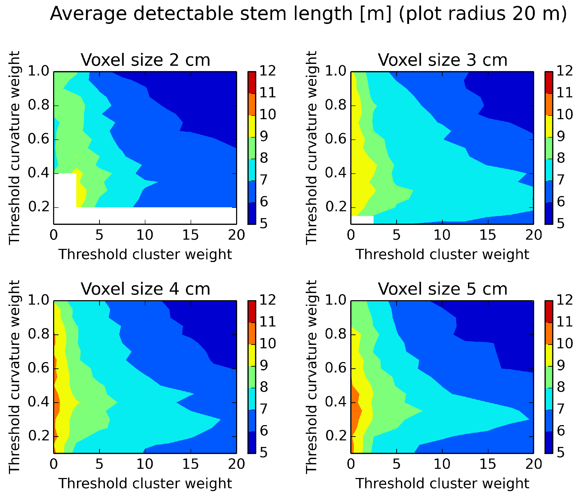
Figure 13.
Average detectable stem length evaluated on a plot of a radius of 20 m and different parameter settings. White areas indicate missing data. Low threshold parameter values give many estimated stem diameters along the tree.
Figure 13.
Average detectable stem length evaluated on a plot of a radius of 20 m and different parameter settings. White areas indicate missing data. Low threshold parameter values give many estimated stem diameters along the tree.
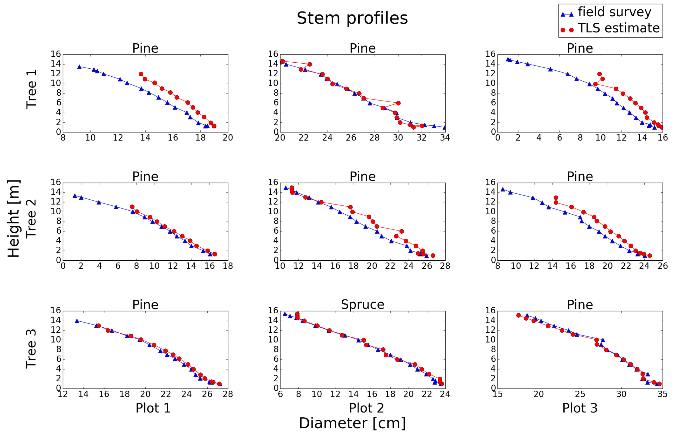
Figure 14.
Stem profiles of the trees in Plots 1–3. The parameter settings used in the stem profile detection method were: voxel size of 3 cm, curvature weight of 0.75 and cluster weight of 15.
Figure 14.
Stem profiles of the trees in Plots 1–3. The parameter settings used in the stem profile detection method were: voxel size of 3 cm, curvature weight of 0.75 and cluster weight of 15.
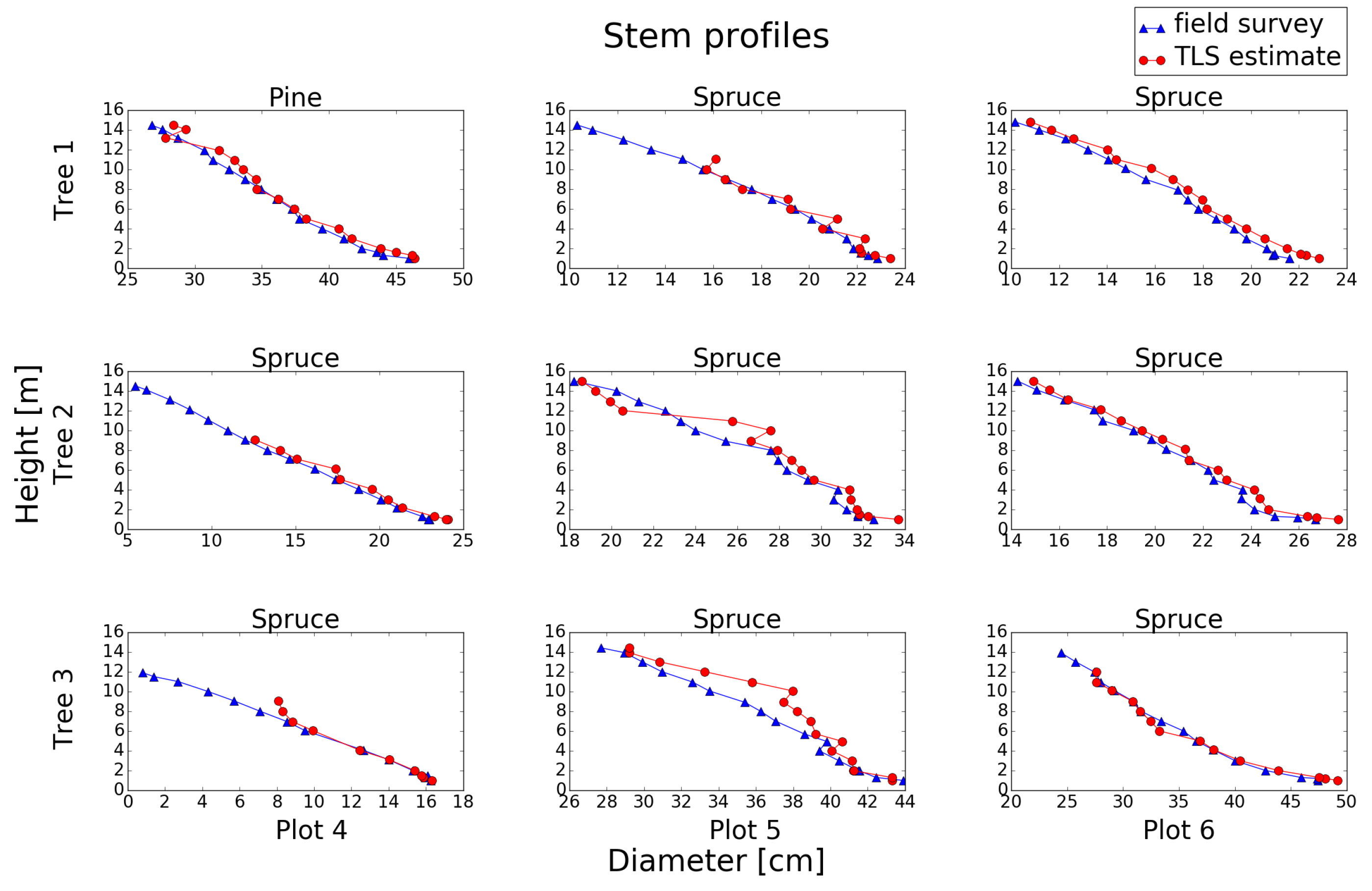
Figure 15.
Stem profiles of the trees in Plots 4–6. The parameter settings used in the stem profile detection method were: voxel size of 3 cm, curvature weight of 0.75 and of cluster weight 15.
Figure 15.
Stem profiles of the trees in Plots 4–6. The parameter settings used in the stem profile detection method were: voxel size of 3 cm, curvature weight of 0.75 and of cluster weight 15.
Figure 16.
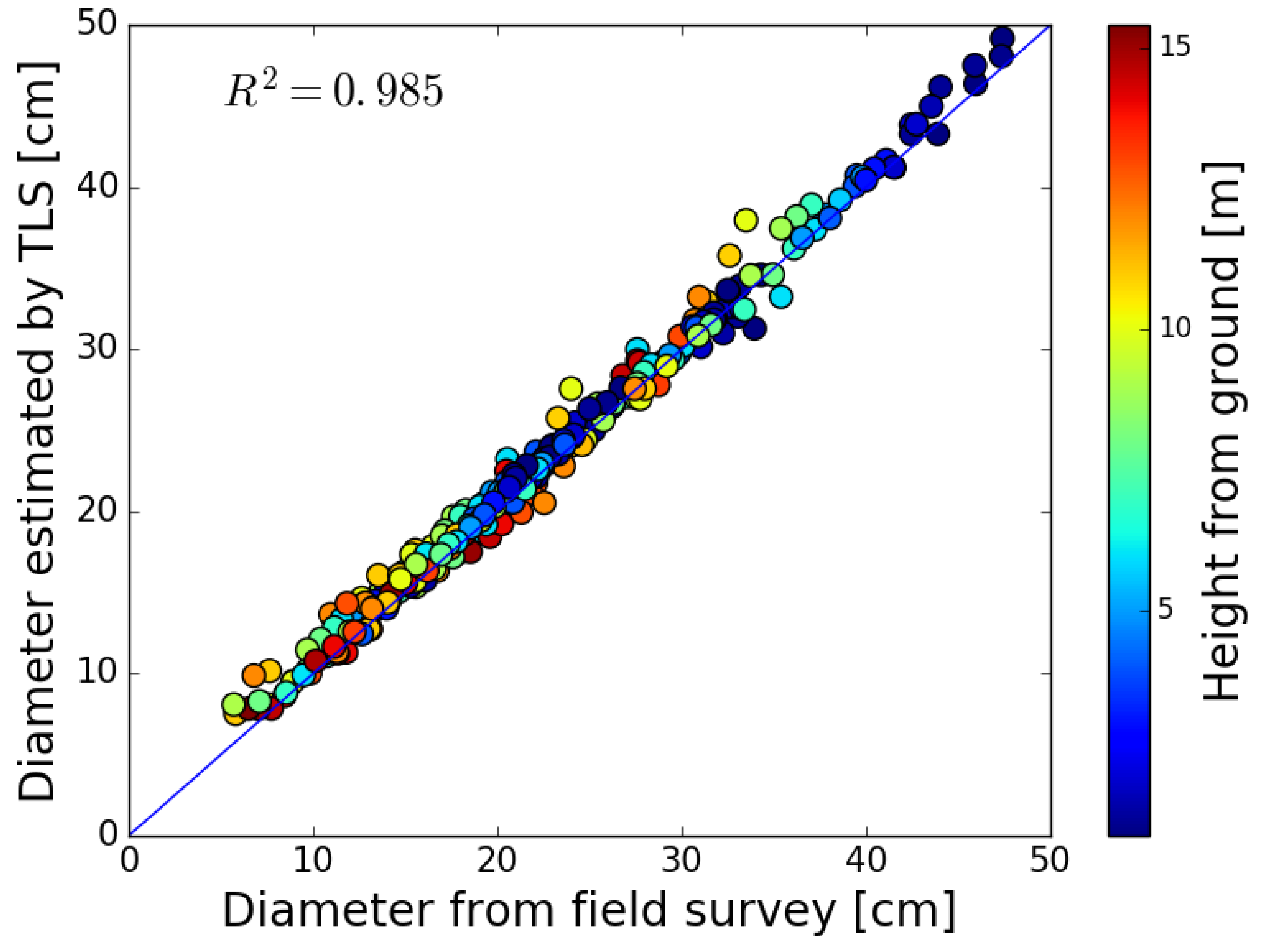
Scatter plot of the stem diameters estimated by TLS versus the stem diameters measured in the field survey for all of the trees in Plots 1–6. The identity line is blue. For stem profile diameters RMSE, bias and omission errors, see
Table 7. The parameter settings used in the stem profile detection method were: voxel size of 3 cm, curvature weight of 0.75 and cluster weight of 15.
Figure 16.
Scatter plot of the stem diameters estimated by TLS versus the stem diameters measured in the field survey for all of the trees in Plots 1–6. The identity line is blue. For stem profile diameters RMSE, bias and omission errors, see
Table 7. The parameter settings used in the stem profile detection method were: voxel size of 3 cm, curvature weight of 0.75 and cluster weight of 15.
Table 1.
Stand average values for the plots used in the stem profile evaluation. The mean tree height was basal area weighted.
Table 1.
Stand average values for the plots used in the stem profile evaluation. The mean tree height was basal area weighted.
| Plot | Pine (%) | Spruce (%) | Mean Tree Height (m) | Basal Area (m2/ha) | Age (Years) |
|---|
| 1 | 100 | 0 | 17.4 | 26 | 109 |
| 2 | 60 | 40 | 18.5 | 29 | 102 |
| 3 | 80 | 20 | 18.8 | 27 | 121 |
| 4 | 90 | 10 | 23.3 | 28 | 145 |
| 5 | 20 | 80 | 23.3 | 37 | 158 |
| 6 | 20 | 80 | 21.6 | 31 | 124 |
Table 2.
Stem profile evaluation trees.
Table 2.
Stem profile evaluation trees.
| Plot | Tree | DBH1 (cm) | DBH2 (cm) | DBH Mean (cm) | Species | Sensor Distance (m) |
|---|
| 1 | 1 | 18.80 | 18.20 | 18.50 | Pine | 10.0 |
| 1 | 2 | 16.20 | 15.90 | 16.05 | Pine | 11.7 |
| 1 | 3 | 25.90 | 26.70 | 26.30 | Pine | 11.6 |
| 2 | 1 | 32.60 | 33.50 | 33.05 | Pine | 16.0 |
| 2 | 2 | 25.70 | 24.90 | 25.30 | Pine | 7.7 |
| 2 | 3 | 22.70 | 23.00 | 22.85 | Spruce | 12.9 |
| 3 | 1 | 14.00 | 15.30 | 14.65 | Pine | 7.6 |
| 3 | 2 | 23.00 | 23.50 | 23.25 | Pine | 10.6 |
| 3 | 3 | 32.60 | 33.70 | 33.15 | Pine | 15.3 |
| 4 | 1 | 43.20 | 44.90 | 44.05 | Pine | 5.1 |
| 4 | 2 | 22.60 | 22.50 | 22.55 | Spruce | 8.9 |
| 4 | 3 | 15.50 | 16.40 | 15.95 | Spruce | 8.8 |
| 5 | 1 | 22.90 | 22.00 | 22.45 | Spruce | 7.6 |
| 5 | 2 | 31.40 | 32.10 | 31.75 | Spruce | 7.9 |
| 5 | 3 | 42.70 | 42.20 | 42.45 | Spruce | 9.3 |
| 6 | 1 | 20.80 | 21.00 | 20.90 | Spruce | 9.5 |
| 6 | 2 | 25.00 | 25.00 | 25.00 | Spruce | 11.3 |
| 6 | 3 | 44.40 | 47.40 | 45.90 | Spruce | 12.4 |
Table 3.
Performance of different algorithms for calculating the flatness of the neighborhood of each point in a point cloud. The cell size is 3 × 3× 3 cm3.
Table 3.
Performance of different algorithms for calculating the flatness of the neighborhood of each point in a point cloud. The cell size is 3 × 3× 3 cm3.
| Algorithm | Radius (cm) | Flatness Ratio RMSE | Time (ms) |
|---|
| Pointwise | 1.86 | - | 5275 |
| Cell | - | 0.261 | 15 |
| Center | 1.86 | 0.179 | 46 |
| Centroid | 1.86 | 0.132 | 48 |
| Pointwise | 2.12 | - | 6399 |
| Cell | - | 0.276 | 15 |
| Center | 2.12 | 0.164 | 51 |
| Centroid | 2.12 | 0.124 | 53 |
Table 4.
Maximum accuracy values for each voxel size and a plot of a radius of 10 m. For each voxel size, there are a number of weight settings from the parameter study that gave equally large maximum accuracy values.
Table 4.
Maximum accuracy values for each voxel size and a plot of a radius of 10 m. For each voxel size, there are a number of weight settings from the parameter study that gave equally large maximum accuracy values.
| Voxel Size (cm) | Cluster Weight | Curvature Weight | Accuracy | Consecutive RMSE (cm) | Length (m) |
|---|
| 2 | 17.5 | 0.60 | 0.878 | 2.2 | 7.9 |
| 2 | 20.0 | 0.60 | 0.878 | 2.1 | 7.5 |
| 3 | 7.5 | 0.75 | 0.902 | 1.8 | 8.4 |
| 3 | 10.0 | 0.75 | 0.902 | 1.5 | 8.1 |
| 3 | 12.5 | 0.75 | 0.902 | 1.3 | 7.5 |
| 3 | 15.0 | 0.75 | 0.902 | 1.2 | 7.0 |
| 3 | 17.5 | 0.75 | 0.902 | 1.2 | 6.6 |
| 3 | 7.5 | 0.85 | 0.902 | 1.9 | 8.0 |
| 3 | 10.0 | 0.85 | 0.902 | 1.6 | 7.6 |
| 3 | 12.5 | 0.85 | 0.902 | 1.3 | 7.0 |
| 3 | 15.0 | 0.85 | 0.902 | 1.2 | 6.9 |
| 3 | 17.5 | 0.85 | 0.902 | 1.2 | 6.5 |
| 4 | 15.0 | 0.75 | 0.900 | 1.0 | 7.2 |
| 4 | 17.5 | 0.75 | 0.900 | 1.0 | 6.9 |
| 4 | 20.0 | 0.75 | 0.900 | 1.1 | 6.8 |
| 4 | 15.0 | 0.80 | 0.900 | 0.9 | 6.9 |
| 4 | 17.5 | 0.80 | 0.900 | 0.9 | 6.8 |
| 4 | 20.0 | 0.80 | 0.900 | 0.8 | 6.7 |
| 4 | 15.0 | 0.85 | 0.900 | 1.1 | 6.8 |
| 4 | 17.5 | 0.85 | 0.900 | 1.0 | 6.6 |
| 4 | 20.0 | 0.85 | 0.900 | 1.0 | 6.5 |
| 5 | 5.0 | 1.00 | 0.900 | 1.4 | 7.5 |
| 5 | 7.5 | 1.00 | 0.900 | 1.4 | 6.8 |
Table 5.
Maximum accuracy values for each voxel size and a plot of a radius of 20 m. For this plot radius only, one weight setting per voxel size from the parameter study gave the maximum accuracy values.
Table 5.
Maximum accuracy values for each voxel size and a plot of a radius of 20 m. For this plot radius only, one weight setting per voxel size from the parameter study gave the maximum accuracy values.
| Voxel Size (cm) | Cluster Weight | Curvature Weight | Accuracy | Consecutive RMSE (cm) | Length (m) |
|---|
| 2 | 12.5 | 0.30 | 0.689 | 2.6 | 6.8 |
| 3 | 5.0 | 0.70 | 0.723 | 2.2 | 7.1 |
| 4 | 12.5 | 0.35 | 0.734 | 1.7 | 7.3 |
| 5 | 2.5 | 0.70 | 0.717 | 2.0 | 8.0 |
Table 6.
Stem profile diameter RMSE and omission errors of the trees in Plots 1–6 at the Svartberget test site for the chosen parameter settings in
Table 4 and
Table 5. The total number of manually-calipered stem profile diameters is 305.
Table 6.
Stem profile diameter RMSE and omission errors of the trees in Plots 1–6 at the Svartberget test site for the chosen parameter settings in Table 4 and Table 5. The total number of manually-calipered stem profile diameters is 305.
| Voxel Size (cm) | Curve Weight | Cluster Weight | No Detected Diameters | Omissions (%) | Profile RMSE (cm) |
|---|
| 2 | 0.30 | 12.5 | 270 | 11.5 | 3.272 |
| 2 | 0.60 | 17.5 | 205 | 32.8 | 5.475 |
| 2 | 0.60 | 20.0 | 188 | 38.4 | 5.485 |
| 3 | 0.75 | 10.0 | 282 | 7.5 | 1.392 |
| 3 | 0.75 | 12.5 | 278 | 8.9 | 1.289 |
| 3 | 0.75 | 15.0 | 274 | 10.2 | 1.104 |
| 3 | 0.75 | 17.5 | 273 | 10.5 | 1.118 |
| 3 | 0.75 | 7.5 | 277 | 9.2 | 1.625 |
| 3 | 0.70 | 5.0 | 282 | 7.5 | 3.799 |
| 3 | 0.85 | 10.0 | 276 | 9.5 | 1.252 |
| 3 | 0.85 | 12.5 | 275 | 9.8 | 1.340 |
| 3 | 0.85 | 15.0 | 272 | 10.8 | 1.393 |
| 3 | 0.85 | 17.5 | 264 | 13.4 | 1.418 |
| 3 | 0.85 | 7.5 | 281 | 7.9 | 2.202 |
| 4 | 0.35 | 12.5 | 289 | 5.2 | 2.552 |
| 4 | 0.75 | 15.0 | 273 | 10.5 | 1.112 |
| 4 | 0.75 | 17.5 | 271 | 11.1 | 1.088 |
| 4 | 0.75 | 20.0 | 267 | 12.5 | 1.027 |
| 4 | 0.85 | 15.0 | 272 | 10.8 | 1.140 |
| 4 | 0.85 | 17.5 | 270 | 11.5 | 1.091 |
| 4 | 0.85 | 20.0 | 266 | 12.8 | 1.013 |
| 4 | 0.80 | 15.0 | 272 | 10.8 | 1.111 |
| 4 | 0.80 | 17.5 | 270 | 11.5 | 1.095 |
| 4 | 0.80 | 20.0 | 266 | 12.8 | 1.016 |
| 5 | 0.70 | 2.5 | 294 | 3.6 | 3.177 |
| 5 | 1.00 | 5.0 | 280 | 8.2 | 2.161 |
| 5 | 1.00 | 7.5 | 273 | 10.5 | 1.138 |
Table 7.
Stem profile diameter RMSE and omission errors for different height spans of the trees in Plots 1–6 at the Svartberget test site. The parameter settings used in the stem profile detection method were: voxel size of 3 cm, curvature weight of 0.75 and cluster weight of 15. The total number of manually-calipered stem profile diameters is 305.
| Height Span (m) | Profile RMSE (cm) | Bias (cm) | Omission (%) |
|---|
| 0.0–2.5 | 1.019 | 0.469 | 0.0 |
| 2.5–5.0 | 0.794 | 0.519 | 0.0 |
| 5.0–7.5 | 0.998 | 0.644 | 0.0 |
| 7.5–10.0 | 0.992 | 0.644 | 0.0 |
| 10.0–12.5 | 1.546 | 1.035 | 7.4 |
| 12.5–15.0 | 1.299 | 0.388 | 35.9 |
| 15.0–17.5 | 0.974 | 0.380 | 35.3 |
| All | 1.104 | 0.627 | 10.2 |
Table 8.
Stem profile diameter RMSE and omission errors for different height spans of the pine trees at the Svartberget test site. The parameter settings used in the stem profile detection method were: voxel size of 3 cm, curvature weight of 0.75 and cluster weight of 15. The total number of manually-calipered stem profile diameters is 153.
| Height span (m) | Profile RMSE (cm) | Bias (cm) | Omission (%) |
|---|
| 0.0–2.5 | 1.104 | −0.004 | 0.0 |
| 2.5–5.0 | 0.859 | 0.505 | 0.0 |
| 5.0–7.5 | 1.215 | 0.949 | 0.0 |
| 7.5–10.0 | 1.103 | 0.812 | 0.0 |
| 10.0–12.5 | 1.392 | 0.993 | 0.0 |
| 12.5–15.0 | 1.445 | 0.564 | 33.3 |
| 15.0–17.5 | 1.159 | 0.244 | 41.2 |
| All | 1.175 | 0.688 | 9.2 |
Table 9.
Stem profile diameter RMSE and omission errors for different height spans of the spruce trees at the Svartberget test site. The parameter settings used in the stem profile detection method were: voxel size of 3 cm, curvature weight of 0.75 and cluster weight of 15. The total number of manually-calipered stem profile diameters is 152.
| Height Span (m) | Profile RMSE (cm) | Bias (cm) | Omission (%) |
|---|
| 0.0–2.5 | 0.967 | 0.745 | 0.0 |
| 2.5–5.0 | 0.715 | 0.533 | 0.0 |
| 5.0–7.5 | 0.706 | 0.327 | 0.0 |
| 7.5–10.0 | 0.866 | 0.476 | 0.0 |
| 10.0–12.5 | 1.709 | 1.083 | 14.8 |
| 12.5–15.0 | 1.084 | 0.165 | 38.9 |
| 15.0–17.5 | 0.787 | 0.493 | 29.4 |
| All | 1.026 | 0.565 | 11.2 |


