Improved Multi-Sensor Satellite-Based Aboveground Biomass Estimation by Selecting Temporally Stable Forest Inventory Plots Using NDVI Time Series

Abstract

Accurate estimates of aboveground biomass (AGB) are crucial to assess terrestrial C-stocks and C-emissions as well as to develop sustainable forest management strategies. In this study we used Synthetic Aperture Radar (SAR) data acquired at L-band and the Landsat tree cover product together with Moderate Resolution Image Spectroradiometer (MODIS) normalized difference vegetation index (NDVI) time series data to improve AGB estimations over two study areas in southern Mexico. We used Mexican National Forest Inventory (INFyS) data collected between 2005 and 2011 to calibrate AGB models as well as to validate the derived AGB products. We applied MODIS NDVI time series data analysis to exclude field plots in which abrupt changes were detected. For this, we used Breaks For Additive Seasonal and Trend analysis (BFAST). We modelled AGB using an original field dataset and BFAST-filtered data. The results show higher accuracies of AGB estimations using BFAST-filtered data than using original field data in terms of R² and root mean square error (RMSE) for both dry and humid tropical forests of southern Mexico. The best results were found in areas with high deforestation rates where the AGB models based on the BFAST-filtered data substantially outperformed those based on original field data (R²_BFAST = 0.62 vs. R²_orig = 0.45; RMSE_BFAST = 28.4 t/ha vs. RMSE_orig = 33.8 t/ha). We conclude that the presented method shows great potential to improve AGB estimations and can be easily and automatically implemented over large areas.

1. Introduction

Through the process of photosynthesis, vegetation absorbs CO₂ from the atmosphere and stores carbon in the biomass of leaves, branches and stems. This can be summarized as aboveground biomass (AGB), defined as the total amount of aboveground living organic matter in vegetation and expressed as oven-dry tons per unit area [1]. Around 50% of dry aboveground biomass is carbon. Therefore, AGB is one of the crucial parameters to assess terrestrial aboveground C-stocks and C-emissions caused by deforestation and forest degradation. Since vegetation biomass affects a range of ecosystem processes such as carbon and water cycling, as well as energy fluxes, accurate AGB information is required for the development of sustainable forest management strategies [2]. Sustainable forest management can contribute to the reduction of carbon in the atmosphere by the decrease of emissions and the increase of carbon storage (carbon sequestration in vegetation). Field measurements of vegetation parameters (e.g., tree height, tree diameter, crown density) that can be further related with AGB are associated with high costs (e.g., labour-intensive and time-consuming) and are limited to point measurements, which may not adequately describe patterns at different spatial scales. Fortunately, rapid advances in information technology have enabled woody vegetation parameters to be estimated from remote sensing. In particular in tropical forests, remote sensing data provides spatially consistent information for areas that are difficult to access.

Synthetic Aperture Radar (SAR) data have been shown to be useful for AGB estimation across the landscape, e.g., [3,4,5,6,7]. Microwave signals have the capability to penetrate the vegetation profile, reflecting the three-dimensional vegetation structure, and are useful for weather-independent applications, as long wavelengths penetrate clouds. The interactions of the radar waves with vegetation elements are determined by their size, shape, and dielectric properties. Long wavelengths (e.g., at P-band and L-band) are more suitable for the retrieval of woody vegetation structure parameters (e.g., stem volume, AGB) because of their ability to penetrate deeper in forest canopies as compared to short wavelengths (e.g., at X-band and C-band) [4,8,9], and thus to interact with large branches (in order of the wavelength) and trunks. A key parameter obtained from SAR data, backscatter intensity, measures the return of energy from a ground object and is determined by the physical (geometry of the object) and electrical (dielectric constant, which is mostly determined by the water content) properties of the target, as well as by the signal properties (e.g., frequency, polarization and angle of incidence of the emitted wave) [10]. A further SAR parameter, interferometric coherence, can be calculated using interferometry techniques (InSAR). Interferometric coherence represents a degree of correlation between two acquisitions. In general, non-forest areas (e.g., urban areas, bare soil), typically stable over time, have high coherence value. Since coherence is typically lower over forests (through an increase of volume and corresponding temporal decorrelation), interferometric coherence can be used for the mapping of forest/non-forest areas [11] as well as for AGB assessment [12,13]. Limitations of radar data for AGB estimation are saturation as well as strong dependence on environmental conditions (e.g., rain fall, and soil moisture conditions). The saturation level of the SAR signal for AGB estimation depends on forest types and wavelengths and varies between 40–150 t/ha for L-band data ([9,14,15,16,17,18]).

Remote sensing data from optical sensors (e.g., Landsat, Moderate Resolution Image Spectroradiometer (MODIS) are partly appropriate for AGB estimation. Optical data are sensitive to vegetation density [19], which relates to AGB and saturates at high biomass values, e.g., [20,21]. Optical data from Landsat and MODIS are attractive as they are freely available and possess long time series. Disadvantages in the use of optical data for AGB estimation are high cloud cover rates over tropics, and strong dependence on environmental, seasonal and acquisition conditions (e.g., solar zenith angle) [22].

The estimation of vegetation parameters (e.g., AGB, vegetation height, growing stock volume) can be improved by the fusing of SAR imagery with optical data (e.g., from Landsat) and complementary information such as altitude [23,24,25,26,27].

For the most commonly used parametric and non-parametric AGB models, calibration data are needed. However, the reference data used for model calibration and product validation can contain inaccurate measurements as well as outdated information [28]. For instance, if field plots were sampled a few years earlier than the remote sensing data acquisition, changes (caused, e.g., by fire or deforestation) within the field plots are likely to occur. Accordingly, these outdated calibration/validation data can lead to a reduction of model prediction performance and thus decrease product accuracy. Time series analysis of remotely sensed data is recognized as a powerful tool to monitor temporal dynamics in vegetation at different scales (from local to global) [29] and can be used to identify, in an automatic way, reference data within which abrupt changes have occurred. The normalized difference vegetation index (NDVI) [30] is a vegetation index based on a combination of red and near-infrared reflectance; it is sensitive to photosynthetically active vegetation and thus often has been used for vegetation monitoring, e.g., [31,32]. Therefore, NDVI time series are one of the important tools to monitor inter-annual and intra-annual variations over a vegetated area [33,34]. There exist a number of long-term NDVI products, which are mostly based on a combination of different sensors. However, due to temporal inconsistency between the sensors, e.g., caused by orbital shift [35], these NDVI products may possess sensor artefacts, which can cause misinterpretations using time series analysis. By a comparison of three NDVI products derived from SPOT-VEGETATION, MODIS, and Advanced Very High Resolution Radiometer (AVHRR), Horion et al. [34] concluded that the MODIS-based NDVI product is more consistent over time than other two products and showed a better potential to detect changes in tree cover in Sahel. Furthermore, MODIS NDVI data do not include platform orbital shift, and possess higher spatial resolution compared to AVHRR- and SPOT-VGT NDVI products.

In this study we investigated whether filtering of calibration data using change detection information obtained from remotely sensed data can improve AGB model performance. This was done by applying Breaks For Additive Seasonal and Trend (BFAST) analysis [36,37] on MODIS NDVI time series data in order to exclude field inventory plots within which abrupt changes were detected. We compared AGB estimates based on original reference data with results based on filtered reference data from the time series analysis. Moreover, due to the fact that canopy density correlates with aboveground biomass, we used the Landsat tree cover (TC) product [38] as an additional predictor layer for SAR-based AGB models. Furthermore, we included altitude from the Shuttle Radar Topography Mission (SRTM) Digital Elevation Model (DEM) in the AGB modelling. We modelled AGB using a different number of input layers, e.g., using SAR backscatter intensities and interferometric coherences separately and together with Landsat TC and SRTM DEM products, and assessed the modelling performance. Our approach was tested over two study sites located in dry and humid tropical forests in southern Mexico.

2. Materials and Methods

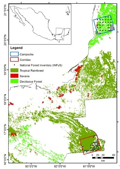
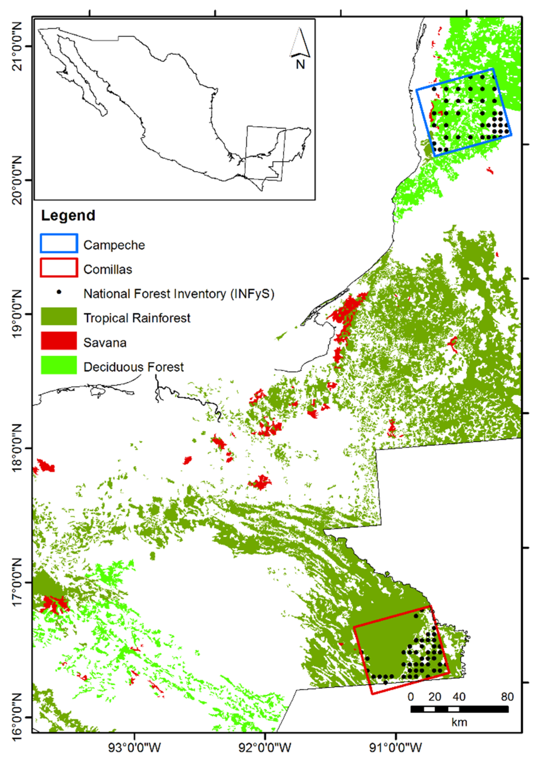
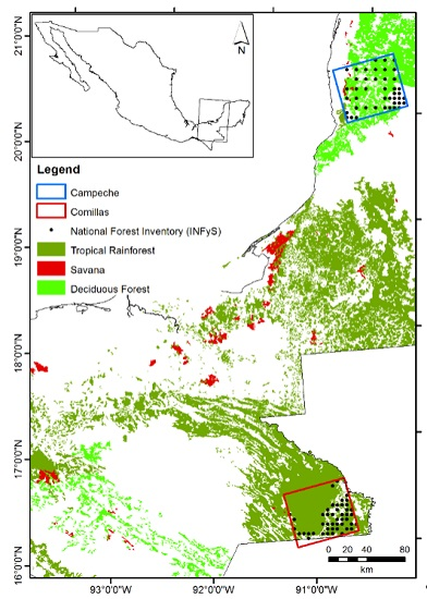
2.1. Study Area

The two study areas are located in the United Mexican States (hereafter Mexico) and are shown in Figure 1 together with the Advanced Land Observing Satellite’s Phased Array type L-band Synthetic Aperture Radar (ALOS PALSAR) footprints (red and blue polygons). The first study area (Figure 1, blue polygon, hereafter Campeche) is partly located in the National Park “Los Petenes-Ría Celestún” in the Campeche and Yucatan federal states. The western part represents a mosaic of mudflats, mixed with mangroves, while the eastern part of the study area is characterized by dry deciduous forests. The climate in the region is tropical sub-humid, with yearly precipitation near 1000 mm, mostly occurring during the summer; the average annual temperature is 26 °C [39]. The surface consists of a coastal plain with some hills with an average elevation of 37.2 m and a standard deviation of 36.8 m. The mean slope is 1.5° with a standard deviation of 1.8°.

The second study area is located in the Lacandon rain forest region in the north-western part of the state of Chiapas (Figure 1, red polygon, hereafter Comillas), and extends over the Montes Azules Biosphere Reserve and the communal lands of Marques de Comillas. The predominant vegetation type in the region is tropical evergreen and semi-evergreen rainforests [40]. The climate is humid tropical with the average annual temperature of 25 °C for the areas below 800 m [41]. Average annual precipitation ranges from 2000 mm to 3500 mm, while the period between June and September is characterized by pronounced rainfall, and the relatively dry period extends between February and April [40,41]. An average elevation in the study area is about 280 m with a standard deviation of 195 m. The mean slope is 5.5° with a standard deviation of 6.4°. Since the region has been treated as a main source for timber [40], it was massively deforested since 1960s [41]. The mean deforestation rates for the Lacandon rain forests (except Marques de Comillas) estimated for the periods 1974–1981 and 1981–1991 were 2.1% and 1.6% per year [41], and 2.1% per year from 1990 to 2010 for the Marques de Comillas region [42].

2.2. Earth Observation Data

2.2.1. SAR Data

ALOS PALSAR data with a wavelength of 23.6 cm were used in this study. The SAR data were available in Single Look Complex (SLC) format acquired in the Fine Beam Single Polarization (FBS) (i.e., single HH (horizontal send-horizontal receive) polarization) and Fine Beam Double Polarization (FBD) (i.e., dual HH and HV (horizontal send-vertical receive) polarizations) modes with an incidence angle of 34.3°. FBS data were collected from December to April between 2007 and 2011 and FBD data were acquired from May to September between 2007 and 2010.

Table 1. Earth observation data used in the study.

Data Sets	Campeche	Comillas
SAR data	L-band backscatter:	L-band backscatter:
	8 FBS (HH polarization)	12 FBS (HH polarization)
	5 FBD (HH/HV polarizations)	9 FBD (HH/HV polarizations)
	4 PALSAR mosaics (HH/HV polarizations)	4 PALSAR mosaics (HH/HV polarizations)
	L-band coherence:	L-band coherence:
	3 FBS pairs (HH polarization)	6 FBS pairs (HH polarization)
	2 FBD pairs (HH/HV polarizations)	4 FBD pairs (HH/HV polarizations)
Optical data	Landsat tree cover 2005
	MODIS NDVI from 2005 to 2011
Ancillary data	SRTM DEM altitude 2000 (1 arc-s)

gives an overview of the number of datasets used in this study. Both FBS and FBD data cover an area of approximately 70 km × 70 km. From the PALSAR SLC data backscatter intensities were calculated (Section 2.4.1). Since some PALSAR data were acquired with a repetition of 46 days, interferometric coherences were calculated from the FBS/FBD data, and used as predictors for AGB modelling.

Furthermore, slope-corrected and orthorectified PALSAR mosaics backscatter data [43] were used as predictor variables in the AGB modelling (Table 1). PALSAR mosaics were available in dual-polarization modes in HH/HV polarizations. The mosaics were built by Japan Aerospace Exploration Agency (JAXA) using PALSAR backscatter data and partly consist of backscatters that differ from the FBS and FBD data described above. The data were downloaded from the JAXA server [44] at 50 m spatial resolution.

2.2.2. Optical Data

As canopy density correlates with AGB, Landsat Tree Cover product (TC) for 2005 Version 3 [38] was used in AGB modelling as an additional explanatory variable (Table 1). Sexton et al. [38] rescaled MODIS Vegetation Continuous Fields (VCF) (University of Maryland, College Park, MD, USA) Tree Cover [45] using circa 2005 Landsat imagery. Landsat TC product exhibits consistency with MODIS VCF product with improvements in discrimination of forest patches in fragmented landscapes [38]. The generated Landsat TC product for 2005 was validated with independent LiDAR measurements collected over Costa Rica, Utah, California and Wisconsin and possessed an average RMSE of 17.4% [38].

For the time series data analysis, MODIS NDVI 16-daily product at 250 m spatial resolution (MOD13Q1) product [46] was used (Table 1). The time series data from January 2005 to December 2011 with the quality flags of 0 (i.e., “good data: use with confidence”) were selected. To gap-fill NDVI time series a linear interpolation between neighbouring values was applied [47]. MODIS NDVI time series data analysis for change detection is further described in Section 2.4.2.

2.3. INFyS Data

The reference INFyS data were collected between 2005 and 2011 by Comisión Nacional Forestal (CONAFOR) of Mexico [48]. The sampling plot consisted of a single circular plot with a radius of 56.42 m covering an area of 1 ha and comprising four sub-plots with an area of 400 m² (0.04 ha). The plot design of INFyS data is similar to the United States Forest Service Forest Inventory and Analysis program (FIA) [49]. From the central sub-plot three further sub-plots at an azimuth of 0°, 120° and 240° were defined. The plots are sampled over the whole country using rectangular grid with a distance between single plots varying from 5 km (in tropical and temperate forests) to 20 km (in arid regions). Within each sub-plot different biophysical parameters (e.g., diameter at breast height, tree height, etc.) were measured. AGB was calculated for each sub-plot using 339 species- and genus-specific allometric models and wood densities [50] and then extrapolated to 1 ha. If more than one model was available, the one with highest R² or with the closest regional relevance was used. Due to the lack of allometries, especially in the tropical areas, also pan-tropical generalized models [1,51] were used.

Over the first study area (Campeche) 28 plots were measured twice, i.e., in 2005 and 2011, and 13 plots were sampled once either in 2005 or in 2011. For the field plots which were measured twice a mean value for two AGB estimates was calculated in order to reduce variations in the data, which can be caused for instance by wrong measurements. We used data from 41 field plots (hereafter original reference data) for AGB modelling (Section 2.4.3) and validation (Section 2.4.4) in Campeche study area. In the Marques de Comillas region three plots have less than four sub-plots and three plots were located on the steep slopes (greater than 15°) and were excluded from the calibration/validation procedure. Twenty-five field plots were sampled twice either in 2005 or in 2011 and 16 once, resulting in 41 plots which were used as original data. Field-based AGB estimates range from 0 to 130 t/ha and from 0 to 170 t/ha in Campeche and Comillas study areas, respectively (Figure 2).

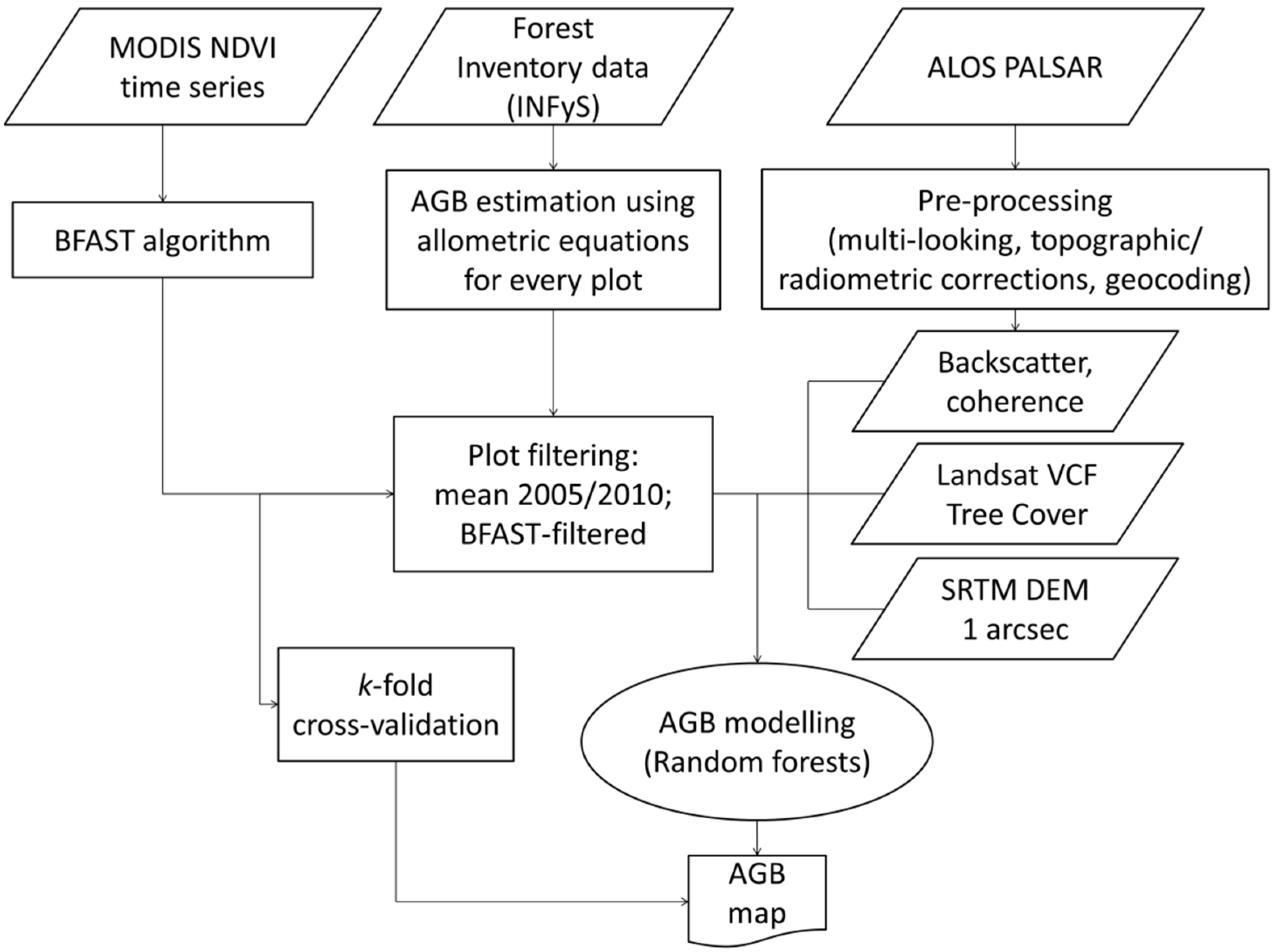
2.4. Processing Steps

This study is based on two main steps. Firstly, we identified forest inventory plots within which abrupt changes were detected using MODIS NDVI time series and BFAST [36,37]. In the next step we used multi-sensor remote sensing data and temporally stable inventory plots to model AGB. In the following subsections a detailed description of each steps is presented (Figure 3).

2.4.1. SAR Data Processing

On the SLC level 1.1 datasets, a multi-look technique was firstly applied. The original spatial resolution of FBS data in radar geometry was 4.68 m × 3.23 m in the range and azimuth directions, respectively. The FBS data were therefore multi-looked by factors 1 and 2 in range and azimuth, resulting in a multi-looked ground resolution of 8.3 m × 6.46 m. Using bilinear interpolation the FBS data were oversampled to a pixel size of 6.25 m × 6.25 m. For FBD data, which original spatial resolution in radar geometry was 9.37 m × 3.23 m in the range and azimuth directions, respectively, multi-looking factors of 1 and 5 in range and azimuth were applied, resulting in a multi-looked ground resolution of 16.63 m × 16.15 m. The FBD data were then oversampled to a pixel size of 12.5 m × 12.5 m using bilinear interpolation. The multi-look images were radiometrically calibrated using a sensor-specific calibration factor (−115 dB). Using SLC scene pairs, interferometric coherences were calculated with similar multi-looking factors described above for FBS and FBD data. The SAR parameters were terrain corrected and geocoded using SRTM DEM. The geocoded SAR parameters were then normalized for topographic effects after Castel et al. [52]. The geocoded and terrain-corrected SAR parameters with different pixel sizes were aggregated to a pixel size of 50 m using a block averaging technique. The aggregation of pixels reduces the influence of speckle noise in the SAR data and the co-registration uncertainty between reference and SAR data [4].

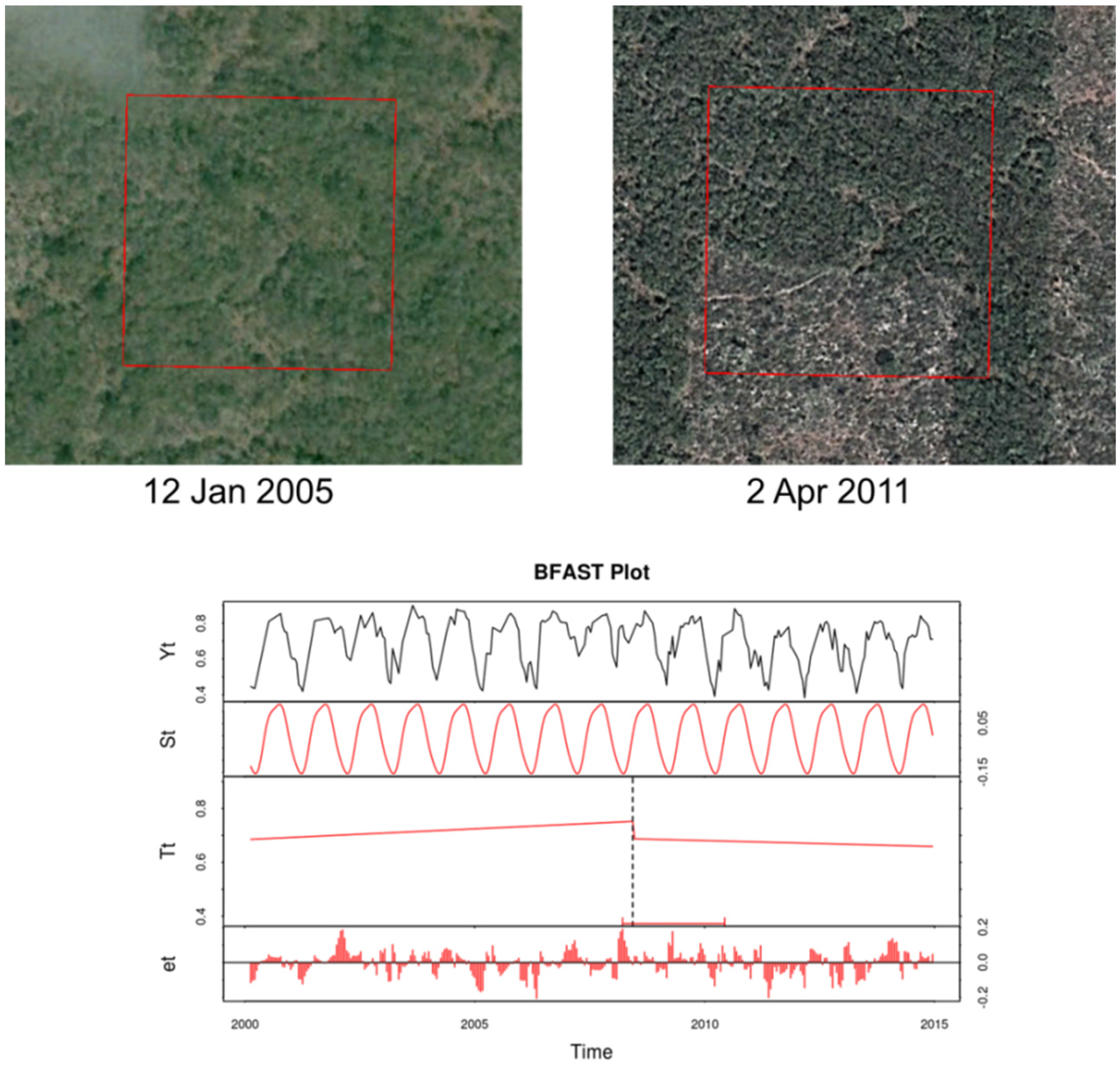
2.4.2. Change Detection Method of NDVI Time Series

To update calibration data and to exclude outdated field plots, we applied BFAST [36,37] to detect plots within which abrupt changes in the remote data have been occurred, indicating potential disturbance or land use change occurring in that particular plot. BFAST is a generic statistically based change detection method developed for time series data, successfully validated for forest change [36] as well as for the detection of phenological events [37]. The algorithm decomposes time series data into trend, seasonal and noise components and detects changes within them. To test whether one or more changes (i.e., breakpoints) in the trend component of time series are occurring, the ordinary least squares (OLS) residual-based MOving SUM (MOSUM) test is applied [53]. By an indication of significant change in the trend component, the breakpoints are estimated using the Bayesian Information Criterion [36]. Verbesselt et al. [36] tested this approach using simulated NDVI time series data with varying magnitude of seasonality and noise as well as using 16 day MODIS NDVI imagery over a forested area in southern Australia. The both tests verified that the algorithm is able to detect and characterize abrupt changes in trend component with robustness against noise and seasonal changes. Furthermore, Dutrieux et al. [54] successfully applied this algorithm on MODIS NDVI data to monitor forest cover loss in a tropical dry forest of Bolivia (overall accuracy of 87%).

We applied BFAST algorithm on MODIS NDVI 16-daily product at 250 m spatial resolution over the field plot areas for a time frame between January 2005 and December 2011. We increased a parameter h (i.e., “the minimal number of observations in each segment divided by the total length of the time series” [55]) in the algorithm to 0.5 (default value 0.1) to reduce the number of breakpoints, i.e., only main big and confident changes were detected. Other parameters have been kept at the default values. In the case of detecting a change (i.e., breakpoint) over a field plot from 2005 to 2011, the field plot was excluded from the AGB model calibration/validation procedure.

2.4.3. AGB Modelling

AGB was modelled for two study areas using a non-parametric model, random forests algorithm (RF) [56]. This machine learning method generates many regression trees with a random selection of predictors at each node as well as with a random subset of samples for each tree with the aim of avoiding overfitting. In order to calculate a single estimate, the predictions of each regression tree are averaged [56]. The RF is a computational efficient and robust non-parametric model and was successfully applied to map vegetation structure metrics (e.g., AGB, tree height) with high retrieval accuracy at large spatial scales, e.g., [19,23,57]. Our random forests were generated with 500 regression trees.

We modelled AGB using three scenarios: (1) a scenario based on original reference data; (2) a scenario based on BFAST-filtered reference data; and (3) a scenario based on random sampling of the same number of observations from the unfiltered data as was used for the BFAST-filtered data. The last scenario was conducted in order to show that the improvements in AGB estimations are due to BFAST-filtering and not due to a reduced number of observations. The random sampling was run 10 times. Furthermore, to investigate the impact of single predictor layers, we modelled AGB using different input variables, e.g., based on PALSAR backscatter intensities, PALSAR interferometric coherences only or in combination with Landsat TC and altitude from SRTM DEM.

2.4.4. k-Fold Cross-Validation

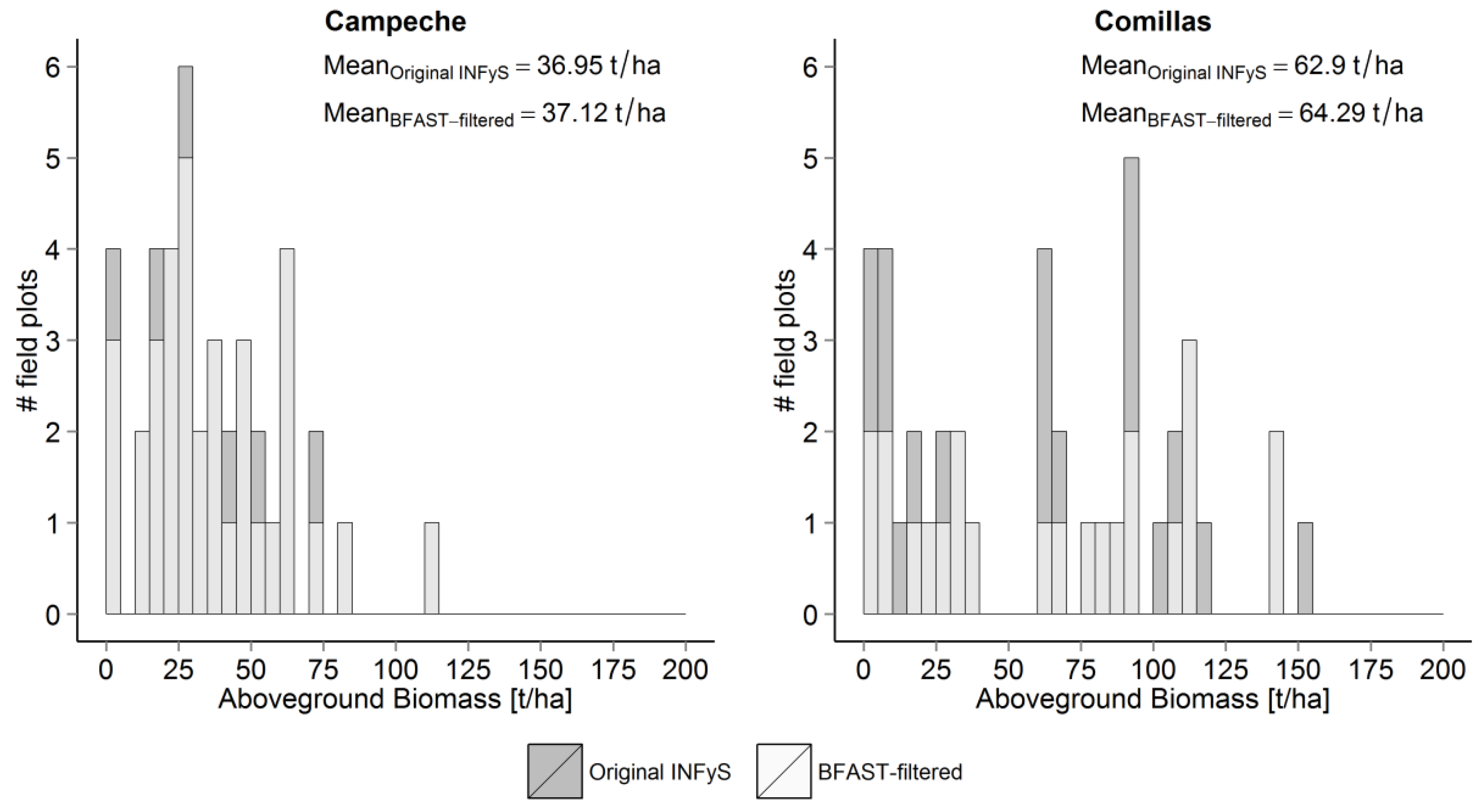
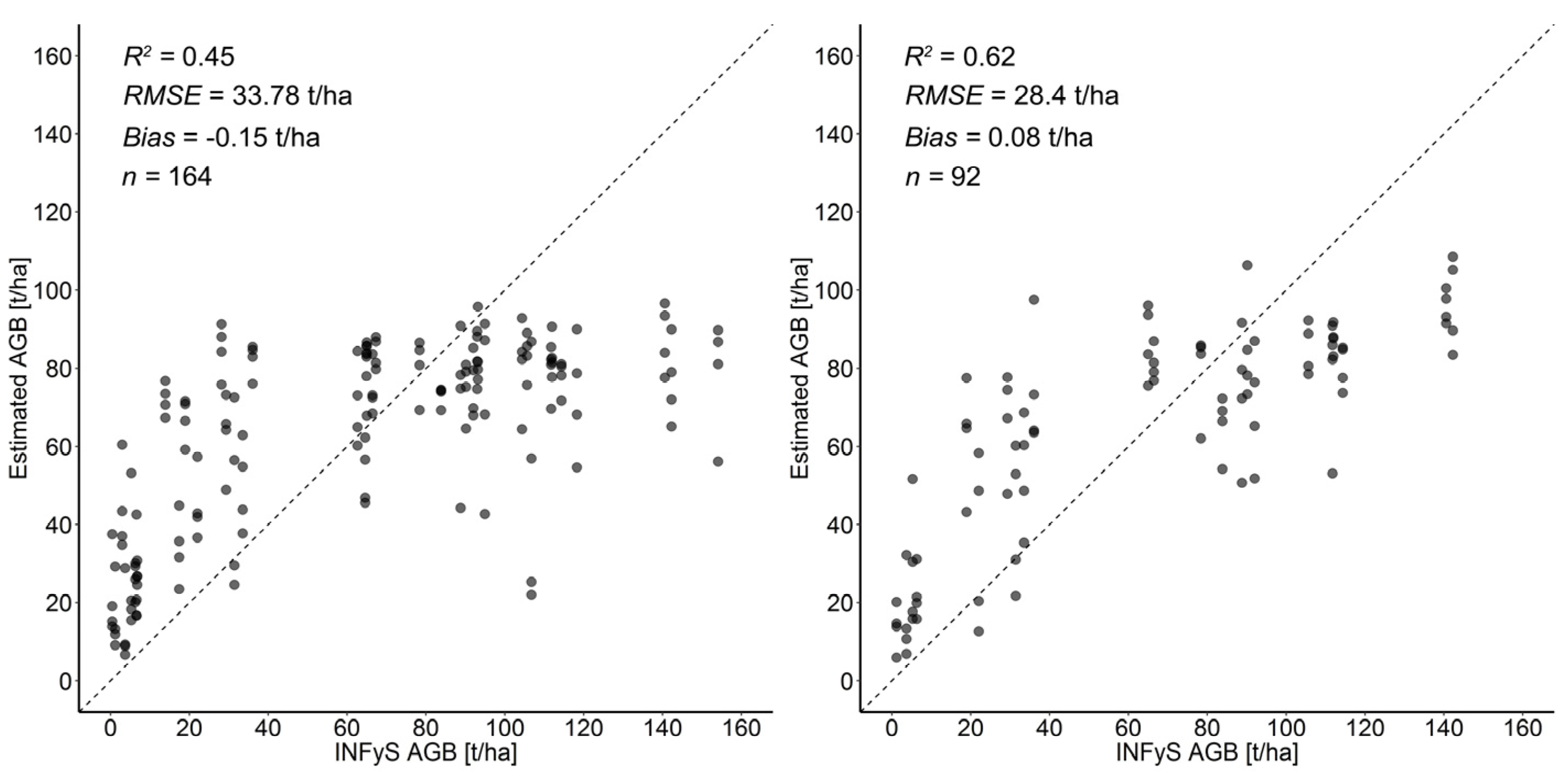
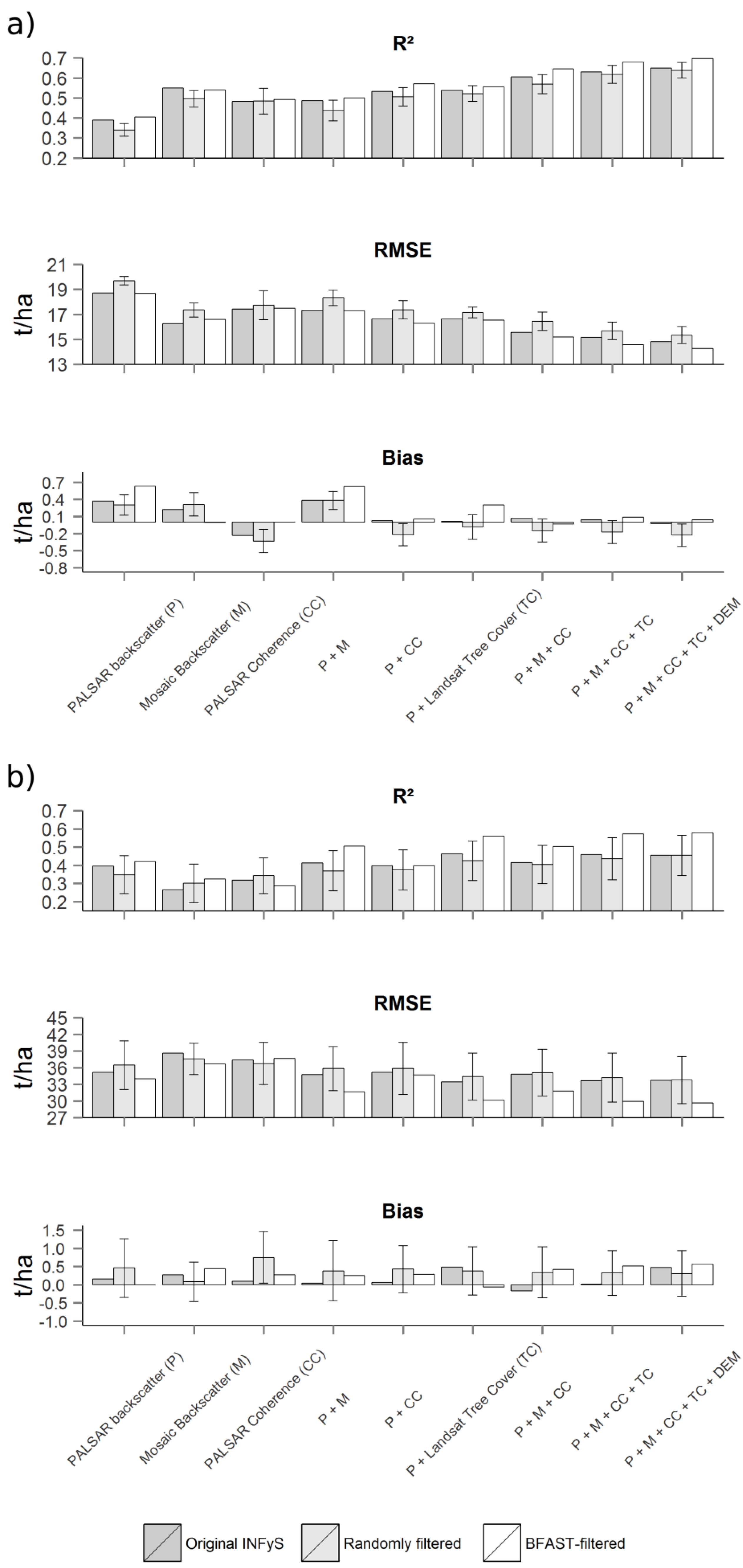
In order to estimate the accuracy of generated products, we applied the k-fold cross-validation technique. Using this technique the dataset is randomly divided in a number of folds (in our case we used 10 folds). One single fold is kept for model validation, while k-1 folds are used for model calibration. This procedure is then repeated k times until all folds have been used as calibration and validation data. All k estimates are finally summarized and a linear regression with the coefficient of determination (R²), root mean square error (RMSE) and bias between predicted and observed data is calculated. The benefit of this validation technique is that each observation will be used once for calibration and validation, so that the dataset is completely validated.

3. Results

The primary objective of this study was to determine whether AGB estimations can be improved by combining multi-sensor remote sensing data and MODIS NDVI time series data. To address this question, we applied the BFAST algorithm on MODIS NDVI time series. The field plots, where abrupt changes were detected, were excluded from the model calibration and products validation. In Figure 4 an example of such a field plot is illustrated, showing Google Earth imagery from 2005 and 2011 over a sample plot in the Campeche region where abrupt changes caused by deforestation have occurred. A corresponding BFAST graph for this field plot, consisting of NDVI values (Yt), and seasonal (St), trend (Tt) and noise (et) components, presents the detection of abrupt changes in the trend component (Figure 4, below).

We modelled AGB using original, BFAST-filtered and randomly filtered reference data as well as using different predictor variables (Section 2.4.3). Using the BFAST algorithm, six and 18 plots were excluded in the Campeche and Comillas study areas, respectively. Accordingly, 35 and 23 BFAST-filtered field plots for Campeche and Comillas were used for AGB modelling. In order to ensure that improvements in AGB estimations are not due to a reduced number of calibration data but due to BFAST, we modelled AGB with 35 and 23 randomly sampled calibration data plots for the Campeche and Comillas study sites, respectively. This random sampling was applied 10 times. The statistics computed using modelled and reference AGB estimates are shown in Figure 5 for the Campeche and Comillas study areas, respectively. The bars by randomly filtered data indicate mean values with the standard deviation shown as error bars. Compared to the results based on the original reference data, AGB estimates based on BFAST-filtered reference data exhibit 8% and 38% higher R² values for the Campeche (R²_orig = 0.65 vs. R²_BFAST = 0.7) and Comillas (R²_orig = 0.45 vs. R²_BFAST = 0.62) study regions, respectively, when using all predictor variables. For the Campeche study area the AGB estimates based on BFAST-filtered data show a slightly lower RMSE compared to the results based on the original reference data. For the Comillas study area the RMSE decreases substantially by around 16% (RMSE_orig = 33.78 t/ha vs. RMSE_BFAST = 28.4 t/ha). AGB estimates based on randomly filtered data showed in most cases the lowest mean R² as well as the highest mean RMSE for both study areas compared to two other scenarios (Figure 5). This indicates that the improvements in AGB estimations are caused not by the reduction of the sample size in the unfiltered data, but by the application of BFAST-filtering. In terms of bias, the results based on BFAST-filtered data showed generally higher bias values than those based on original INFyS data for both test sites.

The reason for this can be that the original data contains lower AGB values (Figure 2), which can introduce a low bias in the training set.

Direct comparisons of the performance of AGB models based on original and BFAST-filtered data and all available predictor layers for the Campeche and Comillas study areas are shown in Figure 6 and Figure 7 (note: 1 ha field inventory plot was covered by four satellite imagery pixels with a spatial resolution of 50 m). In the Campeche study area, only within six field plots abrupt changes were detected and the corresponding number of plots was screened out. This results in a similar distribution of points in the scatterplots with similar statistical metrics (Figure 6). In this region BFAST excluded primarily outlier and mixed pixels in the low AGB range, which have changed over time. In contrast, in the Comillas region, where the deforestation activities have been observed since the 1960s [41,42], 18 field plots were excluded from the calibration data. In Comillas BFAST removed outlier and mixed pixels at low biomass range as well as plots with high biomass (>100 t/ha), indicating deforestation/forest degradation within those field plots (Figure 7). Accordingly the model performance is improved significantly in terms of R² and RMSE. The point distributions along the 1:1 line in Figure 6 and Figure 7 showed typical under-/over-estimation patterns for tree-based regression models, as the predictions of such tree-based models are computed as the average values of the regression trees within each node [56,57]. Moreover, a lower prediction performance at high biomass ranges (over 100 t/ha) for both study sites can be additionally caused by reaching the saturation level of the SAR signal.

To investigate the impact of a single predictor on AGB modelling, we estimated AGB using, e.g., PALSAR backscatter intensities or interferometric coherences separately as well as in combination with further parameters. The inclusion of additional predictor layers (e.g., Landsat TC, SRTM DEM) with SAR products improves AGB estimations and they achieve the highest accuracy (in terms of R² and RMSE) when all predictors are used for all three scenarios: i.e., using original INFyS, BFAST-filtered and randomly filtered data (Figure 5). These results based on the multi-sensor combination are in agreement with previous studies, e.g., [23,25,27].

4. Discussion

The accuracy of AGB estimates based on original data is consistent with the results produced by the authors of [25] in terms of statistical metrics (R² = 0.52 [25] vs. R² = 0.55 (mean for Campeche and Comillas); RMSE = 28.2 t/ha [25] vs. RMSE = 23.8 t/ha (mean for Campeche and Comillas)), while AGB estimates based on BFAST-filtered plots produce more accurate estimates.

The use of MODIS NDVI time series data to detect areas with abrupt changes has the advantage of being fully automated and so can be applied over large areas. Nevertheless, we cannot exclude the confounding influence of the false detection of abrupt changes over field plots, bearing in mind a lower spatial resolution of a MODIS NDVI pixel compared to the plot area (250 m vs. 100 m), and the possible influence of clouds and cloud shadows. Earth observation data at higher spatial resolution (e.g., Landsat) are limited for the calculation of seasonal trends over large areas taking into account cloud cover, SLC-off gaps, as well as restricted access to the whole Landsat archive. However, the launch of the ESA Sentinel-1/Sentinel-2 satellites with free-of-charge imagery opens new perspectives for time series analysis at high spatial resolution. A multi-sensor combination of Landsat and Sentinel-2 time series data as well as fusion with SAR imagery [58] has great potential to enhance time series analysis both in spatial detail and in temporal coverage, potentially leading to a near–real-time forest monitoring system. The inclusion of additional predictor layers (e.g., interferometric coherence, Landsat TC) leads to an improvement of AGB modelling, and the highest prediction performance was achieved when all available predictor variables were used for both test sites. In the Campeche study site, FBS and FBD PALSAR backscatters showed a lower prediction performance compared to four yearly PALSAR mosaic backscatters and interferometric coherences (Figure 5a). The most likely reason is that only five dual-polarized (FBD) backscatter images were available, while one annual PALSAR mosaic consists of different FBD data and may contain additional information. Furthermore, as was shown in Siberia [7], PALSAR coherence was a more important predictor variable than PALSAR backscatter for AGB assessment at a low biomass range (up to 60 t/ha). In the Campeche region, mean field-estimated AGB is around 35–40 t/ha, so L-band interferometric coherences could better explain the AGB distribution than backscatter intensities. However, in the Comillas study site, where a dense stack of L-band backscatters (nine dual-polarized (FBD) together with 12 single-polarized (FBS) backscatters) were available, the backscatter-based AGB model outperformed the models based on PALSAR mosaic backscatters and coherence data (Figure 5b). Moreover, this region exhibits higher AGB distribution (up to 150 t/ha) than Campeche, which can further restrict the use of interferometric coherence in this area. However, SAR-based AGB estimates (i.e., based on PALSAR backscatter, coherence and PALSAR mosaic backscatter) exhibit only slightly lower R² (R²_SAR = 0.65 vs. R²_all = 0.7 for Campeche and R²_SAR = 0.54 vs. R²_all = 0.62 for Comillas), suggesting that L-band SAR data alone would be appropriate for AGB modelling in these tropical dry and humid forests.

The results in the Comillas region are less accurate than in Campeche in terms of statistical metrics due to the several reasons. Firstly, in the Comillas study area tropical rain forests with a higher AGB distribution have occurred, which restricts the use of L-band data in these dense forests. Furthermore, the average annual precipitation in Comillas is more than twice that in Campeche (2000–3500 mm vs. 1000 mm). This leads not only to an increased water content in tree crowns but also to an increased soil moisture, which further limits SAR data for AGB modelling. Finally, the Campeche region is located on a coastal plain with a flat terrain, while in Comillas site hills with partly steep slopes (>15°) are present, which not only restricts SAR data but also can increase geolocation and measurement errors of field data. Collectively, these factors (e.g., denser, moister forests in complex terrain) lead to a decrease of AGB modelling performance in the region.

Moreover, we observed in both study sites an underestimation of AGB modelling for the range higher than 100 t/ha (Figure 6 and Figure 7). From one side it is caused by the L-band signal saturation that occurs in this range. From the other side it is caused by the tree-based regression model itself, as the predictions of the random forest model are computed as the average values of the regression trees within each node [56,57]. Finally, due to the global acquisition strategy implemented by JAXA [59], the L-band cross-pol data (HH/HV polarizations) were acquired between May and September during the rainy season in Mexico. During this season, the water content in vegetation and soil moisture is increased and accordingly limits the use of HV SAR backscatter, which correlates stronger with the vegetation structure than HH SAR backscatter [60,61]. In general, AGB estimations are restricted by possible geolocation inaccuracies of the field data as well as by the fact that the total sampled area of 0.16 ha was extrapolated to 1 ha. However, these sources of errors have an impact on general AGB estimations (i.e., using three scenarios) and not on BFAST-filtering, since the same reference datasets were used for filtering.

5. Conclusions

In this study we showed the improvements in AGB estimations by the filtering of calibration data using change detection information derived from time series analysis of remote sensing data. Our results indicate that MODIS NDVI time series data can be used to identify temporally stable field inventory data, which improves the performance of AGB estimations. The method was evaluated in two study areas in the tropical dry and humid forests of Mexico. Especially the performance of time series analysis was noticeable better in the Comillas region, which possesses high deforestation rates [42]. Moreover, we showed that the improvements in AGB estimations are caused by the application of BFAST-filtering and not by the reduction of the calibration data as shown for randomly selected data. Furthermore, results based on the combination of different predictor layers (i.e., SAR backscatter, interferometric coherence, Landsat TC, SRTM DEM) showed more accurate AGB estimations than those based on a single variable, providing additional explanatory information.

We showed that the filtering of reference data is an important step to improve AGB estimations using remotely sensed imagery. We argue that the presented method shows great potential to enhance AGB estimations and can be easily and automatically implemented over large areas (at national or biome scales).

References

1. Estimating Biomass and Biomass Change of Tropical Forests: A Primer. Available online: http://www.fao.org/docrep/w4095e/w4095e00.htm (accessed on 1 August 2016).
2. Global Forest Resources Assessment 2015. Available online: http://www.fao.org/3/a-i4808e.pdf (accessed on 31 July 2016).
3. Cartus, O.; Santoro, M.; Kellndorfer, J. Mapping forest aboveground biomass in the Northeastern United States with ALOS PALSAR dual-polarization L-band. Remote Sens. Environ. 2012, 124, 466–478. [Google Scholar] [CrossRef]
4. Saatchi, S.; Marlier, M.; Chazdon, R.L.; Clark, D.B.; Russell, A.E. Impact of spatial variability of tropical forest structure on radar estimation of aboveground biomass. Remote Sens. Environ. 2011, 115, 2836–2849. [Google Scholar] [CrossRef]
5. Tanase, M.A.; Panciera, R.; Lowell, K.; Siyuan, T.; Garcia-Martin, A.; Walker, J.P. Sensitivity of L-Band Radar Backscatter to Forest Biomass in Semiarid Environments: A Comparative Analysis of Parametric and Nonparametric Models. IEEE Trans. Geosci. Remote Sens. 2014, 52, 4671–4685. [Google Scholar] [CrossRef]
6. Mitchard, E.T.A.; Saatchi, S.S.; Woodhouse, I.H.; Nangendo, G.; Ribeiro, N.S.; Williams, M.; Ryan, C.M.; Lewis, S.L.; Feldpausch, T.R.; Meir, P. Using satellite radar backscatter to predict above-ground woody biomass: A consistent relationship across four different African landscapes. Geophys. Res. Lett. 2009, 36. [Google Scholar] [CrossRef]
7. Stelmaszczuk-Górska, M.; Rodriguez-Veiga, P.; Ackermann, N.; Thiel, C.; Balzter, H.; Schmullius, C. Non-parametric retrieval of aboveground biomass in Siberian boreal forests with ALOS PALSAR interferometric coherence and backscatter intensity. J. Imaging 2016, 2, 1. [Google Scholar] [CrossRef]
8. Le Toan, T.; Beaudoin, A.; Riom, J.; Guyon, D. Relating Forest Biomass to Sar Data. IEEE Trans. Geosci. Remote Sens. 1992, 30, 403–411. [Google Scholar] [CrossRef]
9. Lucas, R.M.; Moghaddam, M.; Cronin, N. Microwave scattering from mixed-species forests, Queensland, Australia. IEEE Trans. Geosci. Remote Sens. 2004, 42, 2142–2159. [Google Scholar] [CrossRef]
10. Raney, R.K. Radar fundamentals: Technical perspective. In Principles & Applications of Imaging Radar. Manual of Remote Sensing; Henderson, F.M., Lewis, A.J., Eds.; Wiley: New York, NY, USA, 1996; pp. 9–130. [Google Scholar]
11. Luckman, A.; Baker, J.; Wegmüller, U. Repeat-pass interferometric coherence measurements of disturbed tropical forest from JERS and ERS satellites. Remote Sens. Environ. 2000, 73, 350–360. [Google Scholar] [CrossRef]
12. Cartus, O.; Santoro, M.; Schmullius, C.; Li, Z. Large area forest stem volume mapping in the boreal zone using synergy of ERS-1/2 tandem coherence and MODIS vegetation continuous fields. Remote Sens. Environ. 2011, 115, 931–943. [Google Scholar] [CrossRef]
13. Wagner, W.; Luckman, A.; Vietmeier, J.; Tansey, K.; Balzter, H.; Schmullius, C.; Davidson, M.; Gaveau, D.; Gluck, M.; le Toan, T. Large-scale mapping of boreal forest in SIBERIA using ERS tandem coherence and JERS backscatter data. Remote Sens. Environ. 2003, 85, 125–144. [Google Scholar] [CrossRef]
14. Mermoz, S.; le Toan, T.; Villard, L.; Réjou-Méchain, M.; Seifert-Granzin, J. Biomass assessment in the Cameroon savanna using ALOS PALSAR data. Remote Sens. Environ. 2014, 155, 109–119. [Google Scholar] [CrossRef]
15. Mitchard, E.T.A.; Saatchi, S.S.; Lewis, S.L.; Feldpausch, T.R.; Woodhouse, I.H.; Sonké, B.; Rowland, C.; Meir, P. Measuring biomass changes due to woody encroachment and deforestation/degradation in a forest-savanna boundary region of central Africa using multi-temporal L-band radar backscatter. Remote Sens. Environ. 2011, 115, 2861–2873. [Google Scholar] [CrossRef]
16. Saatchi, S.S.; Houghton, R.A.; dos Santos AlvalÁ, R.C.; Soares, J.V.; Yu, Y. Distribution of aboveground live biomass in the Amazon basin. Glob. Chang. Biol. 2007, 13, 816–837. [Google Scholar] [CrossRef]
17. Imhoff, M.L. Radar backscatter and biomass saturation: Ramifications for global biomass inventory. IEEE Trans. Geosci. Remote Sens. 1995, 33, 511–518. [Google Scholar] [CrossRef]
18. Yu, Y.; Saatchi, S. Sensitivity of L-Band SAR Backscatter to Aboveground Biomass of Global Forests. Remote Sens. 2016, 8, 522. [Google Scholar] [CrossRef]
19. Avitabile, V.; Baccini, A.; Friedl, M.A.; Schmullius, C. Capabilities and limitations of Landsat and land cover data for aboveground woody biomass estimation of Uganda. Remote Sens. Environ. 2012, 117, 366–380. [Google Scholar] [CrossRef]
20. Huete, A.R.; Liu, H.Q.; Batchily, K.; van Leeuwen, W. A comparison of vegetation indices over a global set of TM images for EOS-MODIS. Remote Sens. Environ. 1997, 59, 440–451. [Google Scholar] [CrossRef]
21. Huete, A.; Didan, K.; Miura, T.; Rodriguez, E.P.; Gao, X.; Ferreira, L.G. Overview of the radiometric and biophysical performance of the MODIS vegetation indices. Remote Sens. Environ. 2002, 83, 195–213. [Google Scholar] [CrossRef]
22. Steininger, M.K. Satellite estimation of tropical secondary forest above-ground biomass: Data from Brazil and Bolivia. Int. J. Remote Sens. 2000, 21, 1139–1157. [Google Scholar] [CrossRef]
23. Cartus, O.; Kellndorfer, J.; Rombach, M.; Walker, W. Mapping Canopy Height and Growing Stock Volume Using Airborne Lidar, ALOS PALSAR and Landsat ETM+. Remote Sens. 2012, 4, 3320–3345. [Google Scholar] [CrossRef]
24. Basuki, T.M.; Skidmore, A.K.; Hussin, Y.A.; van Duren, I. Estimating tropical forest biomass more accurately by integrating ALOS PALSAR and Landsat-7 ETM+ data. Int. J. Remote Sens. 2013, 34, 4871–4888. [Google Scholar] [CrossRef]
25. Cartus, O.; Kellndorfer, J.; Walker, W.; Franco, C.; Bishop, J.; Santos, L.; Fuentes, J. A National, Detailed Map of Forest Aboveground Carbon Stocks in Mexico. Remote Sens. 2014, 6, 5559–5588. [Google Scholar] [CrossRef]
26. Montesano, P.M.; Cook, B.D.; Sun, G.; Simard, M.; Nelson, R.F.; Ranson, K.J.; Zhang, Z.; Luthcke, S. Achieving accuracy requirements for forest biomass mapping: A spaceborne data fusion method for estimating forest biomass and LiDAR sampling error. Remote Sens. Environ. 2013, 130, 153–170. [Google Scholar] [CrossRef]
27. Rodríguez-Veiga, P.; Saatchi, S.; Tansey, K.; Balzter, H. Magnitude, spatial distribution and uncertainty of forest biomass stocks in Mexico. Remote Sens. Environ. 2016, 183, 265–281. [Google Scholar] [CrossRef]
28. Chowdhury, T.A.; Thiel, C.; Schmullius, C. Growing stock volume estimation from L-band ALOS PALSAR polarimetric coherence in Siberian forest. Remote Sens. Environ. 2014, 155, 129–144. [Google Scholar] [CrossRef]
29. De Jong, R.; Verbesselt, J.; Zeileis, A.; Schaepman, M. Shifts in global vegetation activity trends. Remote Sens. 2013, 5, 1117–1133. [Google Scholar] [CrossRef] [Green Version]
30. Tucker, C.J. Red and photographic infrared linear combinations for monitoring vegetation. Remote Sens. Environ. 1979, 8, 127–150. [Google Scholar] [CrossRef]
31. De Jong, R.; de Bruin, S.; de Wit, A.; Schaepman, M.E.; Dent, D.L. Analysis of monotonic greening and browning trends from global NDVI time-series. Remote Sens. Environ. 2011, 115, 692–702. [Google Scholar] [CrossRef] [Green Version]
32. Ichii, K.; Kondo, M.; Okabe, Y.; Ueyama, M.; Kobayashi, H.; Lee, S.J.; Saigusa, N.; Zhu, Z.; Myneni, R. Recent changes in terrestrial gross primary productivity in Asia from 1982 to 2011. Remote Sens. 2013, 5, 6043–6062. [Google Scholar] [CrossRef]
33. Forkel, M.; Carvalhais, N.; Verbesselt, J.; Mahecha, M.; Neigh, C.; Reichstein, M. Trend change detection in NDVI time series: Effects of inter-annual variability and methodology. Remote Sens. 2013, 5, 2113–2144. [Google Scholar] [CrossRef]
34. Horion, S.; Fensholt, R.; Tagesson, T.; Ehammer, A. Using earth observation-based dry season NDVI trends for assessment of changes in tree cover in the Sahel. Int. J. Remote Sens. 2014, 35, 2493–2515. [Google Scholar] [CrossRef]
35. Prinzon, J.; Brown, M.E.; Tucker, C.J. EMD correction of orbital drift artifacts in satellite data stream. In Hilbert-Huang Transform: Introduction and Applications; Huang, N., Ed.; World Scientific Publishing Co. Pte. Ltd.: Singapore, Singapore, 2005. [Google Scholar]
36. Verbesselt, J.; Hyndman, R.; Newnham, G.; Culvenor, D. Detecting trend and seasonal changes in satellite image time series. Remote Sens. Environ. 2010, 114, 106–115. [Google Scholar] [CrossRef]
37. Verbesselt, J.; Hyndman, R.; Zeileis, A.; Culvenor, D. Phenological change detection while accounting for abrupt and gradual trends in satellite image time series. Remote Sens. Environ. 2010, 114, 2970–2980. [Google Scholar] [CrossRef]
38. Sexton, J.O.; Song, X.P.; Feng, M.; Noojipady, P.; Anand, A.; Huang, C.Q.; Kim, D.H.; Collins, K.M.; Channan, S.; DiMiceli, C.; et al. Global, 30-m resolution continuous fields of tree cover: Landsat-based rescaling of MODIS vegetation continuous fields with lidar-based estimates of error. Int. J. Digit. Earth 2013, 6, 427–448. [Google Scholar] [CrossRef]
39. Flores, J.S.; Espejel, I.C. Etnoflora Yucatense, 3rd ed; Universidad Autónoma de Yucatán: Yucatán, Mexico, 1994. [Google Scholar]
40. De Jong, B.H.J.; Ochoa-Gaona, S.; Castillo-Santiago, M.A.; Ramírez-Marcial, N.; Cairns, M.A. Carbon flux and patterns of land-use/land-cover change in the Selva Lacandona, Mexico. AMBIO J. Hum. Environ. 2000, 29, 504–511. [Google Scholar] [CrossRef]
41. Mendoza, E.; Dirzo, R. Deforestation in Lacandonia (southeast Mexico): Evidence for the declaration of the northernmost tropical hot-spot. Biodivers. Conserv. 1999, 8, 1621–1641. [Google Scholar] [CrossRef]
42. Couturier, S.; Núñez, J.M.; Kolb, M. Measuring Tropical Deforestation with Error Margins: A Method for REDD Monitoring in South-Eastern Mexico. In Tropical Forests; Sudarshana, P., Ed.; Intech: Rijeka, Croatia, 2012; pp. 269–296. [Google Scholar]
43. Shimada, M.; Ohtaki, T. Generating large-scale high-quality SAR mosaic datasets: Application to PALSAR data for global monitoring. IEEE J. Sel. Top. Appl. Earth Obs. Remote Sens. 2010, 3, 637–656. [Google Scholar] [CrossRef]
44. JAXA. New global 25m-resolution PALSAR-2/PALSAR mosaic and Global Forest/Non-forest Map. Available online: http://www.eorc.jaxa.jp/ALOS/en/palsar_fnf/data/index.htm (accessed on 31 July 2016).
45. Dimiceli, C.; Carroll, M.; Sohlberg, R.A.; Huang, C.Q.; Hansen, M.C.; Townshend, J. Annual Global Automated MODIS Vegetation Continuous Fields (MOD44B) at 250 m Spatial Resolution for Data Years Beginning Day 65, 2000–2010, Collection 5 Percent Tree Cover; University of Maryland: College Park, MD, USA, 2011. [Google Scholar]
46. MOD 13-Gridded Vegetation Indices (NDVI & EVI). Available online: http://modis.gsfc.nasa.gov/data/dataprod/dataproducts.php?MOD_NUMBER=13 (accessed on 17 May 2016).
47. Verbesselt, J.; Jonsson, P.; Lhermitte, S.; Aardt, J.V.; Coppin, P. Evaluating satellite and climate data-derived indices as fire risk indicators in savanna ecosystems. IEEE Trans. Geosci. Remote Sens. 2006, 44, 1622–1632. [Google Scholar] [CrossRef]
48. CONAFOR. Inventario Nacional Forestal y de Suelos. Informe 2004–2009; CONAFOR: Zapopan, Mexico, 2012. [Google Scholar]
49. Bechtold, W.A.; Patterson, P.L.; USDA Forest Service, Southern Research Station. The Enhanced Forest Inventory and Analysis Program-National Sampling Design and Estimation Procedures; USDA Forest Service, Southern Research Station: Asheville, NC, USA, 2005; pp. 1–98.
50. CONAFOR. Allometric Modells. Available online: http://www.mrv.mx/index.php/en/mrv-m-3/work-areas/allometric-modells.html (accessed on 27 July 2016).
51. Chave, J.; Andalo, C.; Brown, S.; Cairns, M.A.; Chambers, J.Q.; Eamus, D.; Folster, H.; Fromard, F.; Higuchi, N.; Kira, T.; et al. Tree allometry and improved estimation of carbon stocks and balance in tropical forests. Oecologia 2005, 145, 87–99. [Google Scholar] [CrossRef] [PubMed]
52. Castel, T.; Beaudoin, A.; Stach, N.; Stussi, N.; le Toan, T.; Durand, P. Sensitivity of space-borne SAR data to forest parameters over sloping terrain. Theory and experiment. Int. J. Remote Sens. 2001, 22, 2351–2376. [Google Scholar] [CrossRef]
53. Zeileis, A. A Unified Approach to Structural Change Tests Based on ML Scores, F Statistics, and OLS Residuals. Econom. Rev. 2005, 24, 445–466. [Google Scholar] [CrossRef]
54. Dutrieux, L.P.; Verbesselt, J.; Kooistra, L.; Herold, M. Monitoring forest cover loss using multiple data streams, a case study of a tropical dry forest in Bolivia. ISPRS J. Photogramm. Remote Sens. 2015, 107, 112–125. [Google Scholar] [CrossRef]
55. Breaks for Additive Season and Trend Project! Available online: http://bfast.r-forge.r-project.org/ (accessed on 31 July 2016).
56. Breiman, L. Random Forests. Mach. Learn. 2001, 45, 5–32. [Google Scholar] [CrossRef]
57. Baccini, A.; Laporte, N.; Goetz, S.J.; Sun, M.; Dong, H. A first map of tropical Africa’s above-ground biomass derived from satellite imagery. Environ. Res. Lett. 2008, 3, 045011. [Google Scholar] [CrossRef]
58. Reiche, J.; Verbesselt, J.; Hoekman, D.; Herold, M. Fusing Landsat and SAR time series to detect deforestation in the tropics. Remote Sens. Environ. 2015, 156, 276–293. [Google Scholar] [CrossRef]
59. Rosenqvist, A.; Shimada, M.; Watanabe, M. ALOS PALSAR: Technical outline and mission concepts. Available online: https://www.yumpu.com/en/document/view/48702574/alos-palsar-technical-outline-and-mission-concepts-15mb (accessed on 27 July 2016).
60. Rauste, Y.; Hame, T.; Pulliainen, J.; Heiska, K.; Hallikainen, M. Radar-based forest biomass estimation. Int. J. Remote Sens. 1994, 15, 2797–2808. [Google Scholar] [CrossRef]
61. Watanabe, M.; Shimada, M.; Rosenqvist, A.; Tadono, T.; Matsuoka, M.; Shakil Ahmad, R.; Ohta, K.; Furuta, R.; Nakamura, K.; Moriyama, T. Forest Structure Dependency of the Relation Between L-Band σ0 and Biophysical Parameters. IEEE Trans. Geosci. Remote Sens. 2006, 44, 3154–3165. [Google Scholar] [CrossRef]
Figure 1. Study areas. Forest type information provided by the Instituto Nacional de Estadística y Geografía (INEGI) landcover map series IV.
Forests 07 00169 g001
Figure 2. AGB distribution over Campeche (left) and Comillas (right) study areas before (dark grey bars) and after BFAST-filtering (light grey).
Forests 07 00169 g002
Figure 3. Flow chart of the data processing and analysis steps.
Forests 07 00169 g003
Figure 4. Google Earth imagery from 2005 and 2011 over a field plot (red polygon) showing an example of abrupt changes (above) and corresponding BFAST plot (below) with NDVI values (Yt), and seasonal (St), trend (Tt) and noise (et) components.
Forests 07 00169 g004
Figure 5. R2, RMSE and bias between estimated and observed AGB using different reference data and predictor variables over Campeche (a) and Comillas (b) study areas. P: FBD and FBD PALSAR backscatter; M: PALSAR mosaic backscatter; CC: PALSAR interferometric coherence; TC: Landsat Tree Cover.
Forests 07 00169 g005
Figure 6. Comparisons of observed and predicted AGB estimates based on original (left) and BFAST-filtered (right) NFI data in Campeche study area. Dotted line is the 1:1 line.
Forests 07 00169 g006
Figure 7. Comparisons of observed and predicted AGB estimates based on original (left) and BFAST-filtered (right) NFI data in Comillas study area. Dotted line is the 1:1 line.
Forests 07 00169 g007