Article

Soil Elements Influencing Community Structure in an Old-Growth Forest in Northeastern China

1
The key Laboratory for Forest Resources & Ecosystem Processes of Beijing, Beijing Forestry University, Beijing 100083, China
2
Faculty of Forestry and Forest Ecology, Georg-August-University Göttingen, Büsgenweg 5, Göttingen D-37077, Germany
3
Department of Forest and Wood Science, University of Stellenbosch, Stellenbosch 7600, South Africa
*
Author to whom correspondence should be addressed.
These authors contributed equally to this work.
Forests 2016, 7(8), 159; https://doi.org/10.3390/f7080159
Submission received: 6 May 2016 / Revised: 19 July 2016 / Accepted: 26 July 2016 / Published: 28 July 2016
(This article belongs to the Special Issue Nutrient Cycling and Plant Nutrition in Forest Ecosystems)

Abstract

:
This study uses detailed soil and vegetation data collected in a 30-ha old-growth broad-leaved Korean pine forest to study the effect of soil properties on tree community structures. Spatial distribution patterns are simulated using a homogeneous Poisson process (HomP) and a homogeneous Thomas process (HomT). The simulated distributions are compared with the observed ones to explore correlations between certain tree species and several soil elements. The HomP model shows that all tested tree species are significantly correlated with at least one principal component in the upper-layer soil elements. The HomT model shows that only 36.4% of tree species are significantly correlated with the principal component of at least one upper-layer soil element. This result shows that the impact of dispersal limitation is greater than impact of environmental heterogeneity on species spatial distributions. The spatial autocorrelation of species induced by the dispersal limitation will largely conceal the plant-soil relationships caused by the heterogeneity of soil elements. An additional analysis shows that the elements in the upper soil layer which have the greatest impact on community niche structure are Pb, total phosphorus (TP), total nitrogen (TN), Cu, Cr, Zn and available nitrogen (AN). The corresponding elements in the lower soil layers are Pb, TP, Cu, organic carbon (OC), Mn, total potassium (TK) and AN. Different species seem to be complementary regarding the demands on the available soil resources. The results of this study show that the tree species in the different growth groups have different habitat preferences. Compared with subcanopy and shrub species, the canopy species have more significant correlations with the soil elements.

Graphical Abstract

1. Introduction

The impact of species dispersal and habitat filtering on the species distribution at medium (1–100 km2) and large landscape scales (100–10,000 km2) can be easily quantified if the soil resources of a particular forest community show a mosaic pattern and exhibit obvious heterogeneity characteristics [1], in which case certain habitat factors may have a significant impact on the species spatial distribution [2,3,4]. At the local scale (<1 km2), the pattern induced by a species dispersal limitation is very similar to that induced by the habitat heterogeneity. It is therefore relatively difficult to distinguish between the impact of species dispersal and habitat filtering on a species’ spatial distribution. A considerable amount of evidence shows that the species distribution is often closely correlated with certain soil elements, as well as with the soil texture, terrain features, parent material and other factors at a local scale [5]. Such significant plant-soil relationships occur widely in temperate forests, subtropical forests and tropical forests [5,6,7,8].
Seed dispersal is an important ecological process affecting community structuring. Dispersal limitation will occur when the seeds cannot arrive at a new suitable location, and available evidence shows that species dispersal limitation is often found in the forest communities [9]. However, whether dispersal limitation will have a significant impact on community spatial patterns is still in dispute [10]. Habitat filtering is another important ecological process affecting community assemblage and species coexistence [11,12]. The habitat filtering effect may significantly impact the growth and survival of seedlings. A species adapted to a particular habitat can survive and coexist with other species, while a species which is not adapted to that habitat may be eliminated [13,14]. In tropical and subtropical forests, certain habitat factors such as topography and soil conditions may cause many plant species to show clustered distributions. The spatial distribution of plant species is often highly correlated with certain habitat factors [15,16]. Habitat heterogeneity isolates those species which are unable to coexist into different habitat patches. For example, different species have different competitive capacities in different habitat patches and respectively occupy the patches where they have the strongest competitive capacity [17]. In undisturbed forests, the resource heterogeneity shows a very low contribution to species diversity, while the resource quantity in heterogeneous habitats is the main driving force impacting on the species diversity [18].
Studies involving the relationship between species distributions and environmental factors often consider the topographic variables or habitat types based on specific topographic variables [8,19]. However, the topographical factors are not suitable to replace the soil property for disclosing the impact of environmental factors on the species distribution [20]. Therefore, it is necessary to adopt direct environmental factors such as soil elements in the study of plant-soil relationships [6]. In addition, different tree species contribute differently to the soil nutrient composition through their mycorrhiza and litter. Bonifacio et al. [21] found that the content of organic matter in the soil of a broad-leaved spruce mixed forest was lower than that in a pure spruce forest. Moreover, the organic matter in the local soil layer of the pure spruce forest was obviously enriched, but all of the soil organic matter in the broad-leaved spruce mixed forest was distributed uniformly.
The importance of the soil resource heterogeneity to the maintenance of community diversity has been widely recognized, but the impact of the soil resource quantity on the species distribution has not yet been evaluated systematically. Temperate forests account for a high proportion of the world’s forest resources, and research regarding the relationship between soil resources and species distribution is helpful in revealing the structuring mechanisms of temperate forest communities. This study evaluates the relationship between species spatial distributions and soil resources in an old-growth broad-leaved Korean pine forest community and attempts to answer the following questions: (1) Do the soil elements significantly affect the species spatial distribution in a broad-leaved Korean pine forest? (2) If yes, which soil elements are closely related to the forest community niche structure? In order to determine the actual relationship between the plant and soil elements, we eliminate the disturbance resulting from the species dispersal using specific spatial simulation techniques.

2. Materials and Methods

2.1. Field Data Acquisition

The research area is located within the Jiaohe Forest Experimental Area Administration Bureau of Jilin province, where a temperate continental mountain climate affected by monsoons and an average temperature of 3.7 °C prevails. July is the hottest month, with an average temperature of 21.7 °C. January is the coldest month, with an average temperature of −18.6 °C. The average annual precipitation is 695.9 mm. The soil type is a dark brown forest soil according to the Chinese soil taxonomy [22], with an average depth of 45 cm. In winter, the soil surface freezing time is about 150 days, with a frozen layer depth of 1.0–2.5 m. Because of the strong biological accumulation of the humus layer effect, the soil has high organic carbon content.
In 2010, a 30-ha (500 m × 600 m) research plot was established in a typical old-growth broad-leaved Korean pine forest which is located at 43°57.928’–43°58.214’ N and 127°45.287’–127°45.790’ E, far from urban areas and is virtually unaffected by human disturbance. The altitude of the research plot is 576.03–784.18 m, and the altitudinal difference between the highest and the lowest point is 208 m. All woody plants with a breast height diameter (dbh) exceeding 1 cm were tagged and mapped, their species were identified, and their dbhs, tree heights, crown widths, and heights to live crown were assessed. In this 30-ha observational study, a total of 49,678 woody plants (belonging to 48 species) were recorded. The dominant tree species are Pinus koraiensis, Tilia amurensis, Fraxinus mandshurica, Ulmus laciniata and Acer mono.
A combination of systematic and random sampling was used to assess soil properties. We randomly selected one direction from the eight directions around each 40 m × 40 m grid intersection and then randomly selected two distances from 2 m, 8 m and 15 m distances to form three combinations (2 m and 8 m, 2 m and 15 m or 8 m and 15 m) in the selected direction (see [23] for a detailed description of this approach). Finally, a total of 540 sample points were obtained in the 30-ha plot. The plant root system in the plots was mainly concentrated in the 0–20 cm soil layer, especially in the upper 0–10 cm layer, where the root system was dominant. Therefore, soil samples were taken from the upper (0–10 cm) and lower soil layer (10–20 cm) at each sample point and 18 soil variables were assessed: available nitrogen (AN), total nitrogen (TN), available potassium (AK), total potassium (TK), available phosphorus (AP), total phosphorus (TP), organic carbon (OC), pH, Cu, Ni, Cd, As, Pb, Zn, Mo, Cr, Mn and Mg. We used ammonium nitrogen-indophenol blue colorimetry to measure the content of available nitrogen; the hydrochloric acid-ammonium fluoride method to assess available phosphorus; the ammonium acetate extraction method to assess available potassium; the Kelvin heating digestion method to assess total potassium, and the high-temperature external-heat potassium dichromate oxidation method to assess organic carbon. Heavy metal elements were extracted using the Mehlich3 general extracting agent. Concentrations were assessed using inductively coupled plasma atomic emission spectrometry (ICP-AES). The above experiments were carried out according to the recommendations of the China Soil Council [24].

2.2. Relationship between Species Distribution and Soil Elements

Principal component analysis (PCA) was used to identify several composite factors representing various original variables by means of the dimensionality reduction method, and to allow these composite factors to retain the greatest possible amount of information for a large number of original variables. These composite factors had to be mutually unrelated. The 18 soil variables used in this paper have a very high correlation, so there is also a serious multicollinearity problem. In order to compress and extract the main information of the soil elements, principal component analysis was used for these soil elements and the pH values.
The Monte Carlo method was used to simulate species spatial distributions. We assume that the heterogeneous spatial distribution of the soil elements causes specific species distribution patterns. To evaluate this assumption, we applied two spatial point process models, the homogeneous Poisson process (HomP) and the homogeneous Thomas process (HomT) for simulating specific spatial distributions. The homogeneous Poisson process (HomP) simulates a completely random spatial species distribution and is used to test the significance of the plant-soil correlation. The homogeneous HomP thus assumes that all individuals of a certain plant species are randomly distributed in the plots. However, most of the tree species are not randomly distributed, thus it is necessary to consider a non-random process [24]. Therefore, we also used a homogeneous Thomas process (HomT) to simulate the autocorrelation of the species spatial distribution, which may be the result of dispersal processes [25,26,27]. The Poisson process model is usually expressed as Equation (1):
ρ ( μ ) = α · exp ( z 1 : k ( μ ) β 1 : k T )
When ρ ( μ ) is a constant, the point pattern is represented by a homogeneous Poisson process (completely random); z 1 : k ( μ ) is the function of environment variables where μ is the location of a point; α is the average density of the species distribution and β 1 : k T are the coefficients.
The homogeneous Thomas process is usually expressed by Equation (2):
ρ c ( μ ) = α k ( μ c ; δ )
where the parameter c defines the location of the parent tree, and k ( μ c ; δ ) defines the dispersal model of the offspring around the parent trees.
The spatial point process model was used to simulate the distribution pattern of each species in the observational study area [28]. For each species, there are 1000 distribution maps, including 999 simulated maps and one observed species map. The simulated species distribution maps were then matched with the principle components (PCs) distribution maps of the soil elements. The Pearson coefficient between each simulated species distribution and the PC distribution map among the 40 m × 40 m square cells were calculated. Thus, the 95% confidence interval can be calculated based on 999 Pearson coefficients. When the Pearson coefficient between the observed species distribution and the PCs is greater than the upper limit of the 95% confidence interval, then the relationship between the species distribution and the PCs of the soil elements represents a significant positive correlation. The correlation will be negative if the Pearson coefficient between the observed species distribution and the PCs is smaller than the lower limit of the 95% confidence interval. Alternatively, the correlation will be non-significant.
To ensure reasonable sample sizes, the analysis was limited to the 33 most abundant species (Table S1) which are represented by at least 30 individuals in the study area. In accordance with the potential maximum height (hmax), the tree species were assigned to one of three groups: canopy species (hmax ≥ 15 m), subcanopy species (5 m ≤ hmax < 15 m) and shrub species (hmax < 5 m). The 33 species include 23 canopy species, 5 subcanopy species and 5 shrub species.
The Canonical Correspondence Analysis (CCA) was used to study the relationship between the species composition and the soil environment. The species composition was expressed by a species-site matrix, and the soil environment was expressed by 18 soil elements.
The ecological niche breadth, which reflects the degree of adaptation to different environments, is reciprocal to the degree of ecological specialization [29]. In this study, we evaluate Levins’ ecological niche breadth of tree species represented by at least 30 individuals [30], and test the degree of ecological specialization of each species with regard to the soil elements. The Levins’ ecological niche breadth indicator formula is specified in Equation (3):
B i = ( N ij ) 2 / ( N ij 2 )
where Bi is the ecological niche breadth of species i, and Nij is the resource value in the j'th resource grade for species i. In order to evaluate the overall impact of each soil variable on the community niche structure, a boxplot for the ecological niche breadth of all studied species was drawn for each soil variable.
All calculations were performed using the R statistical software [31]. The principal component analysis was implemented using the “vegan”, “ade4”, “gclus” and “ape” packages.

3. Results

The difference in the species compositions among the 40 m × 40 m cells was significantly correlated to the difference in the average concentrations of soil elements in those cells for both the upper and the lower soil layer. The CCA ordination analysis regarding soil nutrient and community composition shows that most soil variables are significantly correlated with the CCA ordination axes (Figure 1, Table 1). However, some soil elements show similar effects according to the lengths and directions of the soil nutrient vectors. Surprisingly, major soil elements (such as N, P and K) do not show a stronger influence than the metal elements (such as Ni, As and Mg) in both soil layers. The same nutrient shows a consistent direction in both soil layers, but the nutrient vectors in the upper soil layer are longer than those in the lower layer (Figure 1).
As soil nutrient variables are significantly correlated with each other (Table S2), we obtained a group of optimum orthogonal unit vectors based on principal component analysis. The first four PCS (PC1, PC2, PC3 and PC4) are not related to one another and jointly explain 53%–54% of the variation in soil elements in the two soil layers. In the two layers, the first principal component (PC1) accounts for 20.3%–21.9% of the variation in soil nutrient concentrations, while the second (PC2) accounts for 11.3%–14.1%. The third principal component (PC3) accounts for 10.7%–10.9% and the fourth (PC4) for 8.9%–9.1% (Table 2).
PC1 is the most important principal component, reflecting the contribution of the metal elements. In the upper soil layer, PC1 shows a positive correlation with Pb, and a negative one with other elements. In the lower soil layer, PC1 has negative correlations with all metal elements except Pb. The loading values of each soil nutrient variable in PC3 show a large difference. PC3 exhibits a negative correlation with most soil variables in the upper soil layer, but a positive one with most soil variables in the lower soil layer. PC2 and PC4 together represent all the information on various soil elements.
When the Monte Carlo method was used to test the relationship between different principal components and species distributions, most species show a significant correlation with the principal components. The difference in species showing significant correlation with the PCs before and after eliminating rare species (n < 30) is minor. Only very few (1–3) rare species show significant correlations with the soil elements (Table 2).
When testing the tree species-soil relationships, four PC axes are used, which replace the individual soil elements to reduce the testing frequency. The HomP model was used to establish the confidence interval and to test whether the species distribution is closely related with the soil elements represented by the PCs. All studied tree species show a significant correlation with at least one principal component of soil elements in the upper soil layer, while 87.9% of the species are significantly related to at least one principal component of elements in the lower soil layer. The HomT model eliminates the effect of the species dispersal limitation, and the results show that only a few tree species exhibit a preference for particular soil elements. A total of 12 tree species are significantly related to at least one principal component of elements in the upper soil layer (accounting for 36.4% of all studied tree species), and 10 tree species are significantly related with at least one principal component of elements in the lower layer (accounting for 30.3% of all studied tree species). The results between the HomT and HomP models are very different. We assume that the spatial autocorrelation of species distributions induced by the dispersal limitation may confound the true plant-soil relationships induced by the spatial heterogeneity of soil elements (Table 3 and Table 4).
Significant species-soil relationships show up mainly for the canopy species. A total of 39.1% of canopy species (14 of 23 species) are significantly related to the PCs of soil elements in the upper soil layer, while 34.8% of canopy species (14 of 23 species) are significantly related to the PCs of soil elements in the lower soil layer. Two out of five subcanopy species show significant correlations with the PCs of soil elements in the upper soil layer, and only one out of five subcanopy species shows significant correlations with the PCs in the lower soil layer. Only one out of five shrub species shows significant correlations with PC3 of soil elements in the upper soil layer and with PC2 and PC4 of elements in the lower soil layer (Table 5).
The soil nutrient variables are highly correlated with each other (Table S2). It is thus difficult to evaluate the relative importance of individual soil elements in a community niche structure. We calculated the ecological niche breadth of all species for individual soil nutrient gradients and conclude that the smaller ecological niche breadth indicates a higher specialization degree of particular focal species. When the ecological niche breadth is relatively small, plant species show a weak adaptability to the variations in soil properties. Thus, the smaller the niche breadth for a given soil variable, the greater is the effect of that soil variable on the niche structure of the community. The soil elements which have the largest impacts on the community niche structure are Pb, TP, TN, Cu, Cr, Zn and AN in the upper soil layer and Pb, TP, Cu, OC, Mn, TK, AN, TN, Zn and Cr in the lower layer (Figure 2). The ecological niche breadths of AK, TK, AP, OC, AN, TN, Ni and pH show significant differences between the two soil layers. These nutritional elements, which are represented differently in the two soil layers (Table S4), are important for plant growth.

4. Discussion

A particular community pattern involves specific ecological processes, and a particular process in turn represents the cause and driving force of many different patterns. Previous studies have shown that the old-growth broad-leaved Korean pine forest exhibits a strong dispersal limitation [32]. The joint effects of environmental heterogeneity and dispersal limitation can more effectively explain the species-area relationships and β diversity in the old-growth broad-leaved Korean pine forest [33]. Our study extracted four principal components to express the spatial variation of soil variables. Each principal component reflects different combinations of the soil characteristics. PC1 indicates the spatial variation of metal elements in soils such as Cu, Ni, Cd, As, Pb, Zn, Mo, Cr, Mn, Mg, while PC2, PC3 and PC4 indicate the spatial variation of the nutrients (nitrogen, phosphorus, potassium, organic carbon) and soil pH.
A species distribution simulation using a spatial point process model can directly evaluate the relationships with the nutrient PCs. The plant-soil relationships tested by the homogeneous Thomas model are less indicative than those tested by the homogeneous Poisson model: they are reduced by 63.6% in the upper soil layer, and by 57.6% in the lower layer. True effects of environmental filtering on the species distribution are reduced after eliminating spatial autocorrelation induced from a dispersal process. Therefore, we can conclude that the dispersal-limitation effect on a particular species distribution is greater than the effect of the environmental heterogeneity.
Previous studies have shown that soil elements strongly affect vegetation patterns in tropical and temperate forest communities [34,35,36,37]. Paoli et al. found that the spatial distributions of 18 out of 22 tree species in a tropical forest community were significantly associated with soil elements, especially with P, Mg and Ca [38]. They argued that dispersal and niche processes jointly determine mesoscale beta diversity in a Bornean Dipterocarp forest. John et al. [7] detected an effect of soil elements on the spatial distribution of particular tree species in three diverse neotropical forest plots. They found that the spatial distributions of 36%–51% of all the tree species in these plots show strong associations with soil nutrient distributions. B and K in their BCI plot, Ca and Mg in the Yasuni plot and K, P, Fe and N in the La Planada plot showed the strongest effects on community niche structure [7].
In a subtropical broad-leaved forest community, spatial heterogeneity of soil elements was associated with distributions of 88.2% (90 out of 102 species) of tree species after controlling the effects of dispersal limitation. The soil factors most strongly influencing species distributions were TC, TN, TP, K, Mg, Si, soil moisture and bulk density [6]. Our results showed that TP, TN, AN in the upper soil layer and TP, TK, TN, AN in the lower soil layer strongly affect species distributions. Nitrogen, phosphorus and potassium are the essential mineral elements for plant growth, as well as being rather limited soil elements, and their concentration directly affects plant growth and survival [39,40]. The variation coefficient of AN, AP, AK, TN, TP and TK in the broad-leaved Korean pine forest ranges from 0.16 to 0.44, and shows obvious spatial heterogeneity (Table S3). When the quantity of nitrogen, phosphorus and potassium in the habitat cannot meet the plants’ demands, they will become important limiting factors for plant growth.
Metal elements show consistent effects on community structure in the two soil layers. Pb, Cu, Cr and Zn in both the upper and lower soil layers strongly affect the community niche structure of the old-growth forest. Previous studies have shown that metal elements have important effects on the growth, development and breeding of plants. Cu is a cofactor influencing the structure and catalytic compounds of proteins and enzymes and is thus essential for the normal growth and biochemical processes. However, excessive Cu will produce a large number of free radicals and malondialdehyde (MDA), causing metabolic disturbances and inhibiting plant growth [41].
Zn is an active cofactor for a large number of enzymes related to the metabolism of DNA transcription, protein, nucleic acid, carbohydrate and lipids [42,43]. Furthermore, Zn is the essential microelement for any living body, and Zn deficiency will cause a series of nutrition problems in plants. Pb is not an essential element and may cause enzyme function disorders, generating active oxygen in plant tissue cells, which will lead to membrane lipid peroxidation, and change the related enzymatic activity of active oxygen metabolism [44,45], which finally affects biochemical processes and the morphological structure of plants [46]. Cr is not an essential element, but may also affect plant growth and development. A high concentration of Cr may inhibit the root cell differentiation of plants, block water absorption, and have a toxic effect, while a low concentration of Cr can promote the growth of roots and root hairs, increase the cortical tissue layers in the roots, and thus facilitate plant growth [47,48]. A low concentration of Cr will also promote the formation of chlorophyll, while a high concentration will inhibit the formation of chlorophyll [49,50]. Mn in the lower soil layer has an especially severe impact on our community niche structure. Mn is an essential element in the PSII oxygen evolution complex [51,52,53], and its role is to realize water splitting in the reaction center of PSII and to provide electrons to the electron transfer chain as part of thylakoid coupling [54]. Therefore, an Mn deficiency will decrease the photosynthetic capacity of the leaves [55].
Different species groups were formed in accordance with their visible properties. Plant species usually belong to the same growth group under similar environmental conditions, which is the result of adaptive convergence [56]. Plant species in different growth groups have shown different soil habitat preferences in a subtropical forest plot. Only five shrub species were significantly related to the four soil property principal component axes, while most of the canopy species and subcanopy species were significantly related to 1–2 principal component axes [6]. Our results show that the tree species in the different growth groups have different habitat preferences. Compared with subcanopy and shrub species, the canopy species have more significant correlations with the PCs of the soil elements. In addition, different canopy species also show different soil preferences. Canopy species play a dominant role in structuring the forest community. Intense competition will occur when different tree species have similar demands for specific soil resources and some members of a species with weak competitive strength may die. On the other hand, the demands of different tree species on available soil resources may be complementary, which facilitates the full utilization of existing resources and the coexistence of species.

5. Conclusions

This work evaluates plant-soil correlations by comparing simulated the spatial distributions of tree species with observed ones in a large forest observational study. The impact of dispersal limitation is greater than impact of environmental heterogeneity on species spatial distributions. The spatial autocorrelation of species induced by the dispersal limitation will largely conceal the plant-soil relationships caused by the heterogeneity of soil elements. Certain elements in the upper and lower soil layers were identified to influence community niche structure. Tree species in different growth groups have different habitat preferences. Compared with subcanopy and shrub species, the canopy species have more significant correlations with the soil elements.

Supplementary Materials

The following are available online at www.mdpi.com/1999-4907/7/8/159/s1, Table S1: Number of individuals of the 33 most abundant species in the 30-ha study area, Table S2: Pearson’s correlations among soil nutrients and pH values, Table S3: Variation coefficients of soil variables within the study area, Table S4: Descriptive statistics of the soil variables.

Acknowledgments

This research is supported by the Fundamental Research Funds for the Central Universities (2015ZCQ-LX-03), the State Key Program of National Natural Science Foundation of China (41330530) and the 12th five-year National Science and Technology plan of China (2012BAC01B03).

Author Contributions

W.X. and J.W. analyzed the data and wrote the manuscript. C.Z. and K.G. modeled and interpreted the results. X.Z. and M.H. performed the laboratory experiments.

Conflicts of Interest

The authors declare no conflict of interest. The founding sponsors had no role in the design of the study; in the collection, analyses, or interpretation of data; in the writing of the manuscript; and in the decision to publish the results.

References

  1. Tuomisto, H.; Ruokolainen, K.; Aguilar, M.; Sarmiento, A. Floristic patterns along a 43-km long transect in an Amazonian rain forest. J. Ecol. 2003, 91, 743–756. [Google Scholar] [CrossRef]
  2. Thessler, S.; Ruokolainen, K.; Tuomisto, H.; Tomppo, E. Mapping gradual landscape-scale floristic changes in Amazonian primary rain forests by combining ordination and remote sensing. Glob. Ecol. Biogeogr. 2005, 14, 315–325. [Google Scholar] [CrossRef]
  3. Slik, J.W.; Raes, N.; Aiba, S.I.; Brearley, F.Q.; Cannon, C.H.; Meijaard, E.; Nagamasu, H.; Nilus, R.; Paoli, G.; Poulsen, A.D.; et al. Environmental correlates for tropical tree diversity and distribution patterns in Borneo. Divers. Distrib. 2009, 15, 523–532. [Google Scholar] [CrossRef]
  4. Clark, D.B.; Olivas, P.C.; Oberbauer, S.F.; Clark, D.A.; Ryan, M.G. First direct landscape-scale measurement of tropical rain forest leaf area index, a key driver of global primary productivity. Ecol. Lett. 2008, 11, 163–172. [Google Scholar] [CrossRef] [PubMed]
  5. Gleason, S.M.; Read, J.; Ares, A.; Metcalfe, D.J. Species-soil associations, disturbance, and nutrient cycling in an Australian tropical rainforest. Oecologia 2010, 162, 1047–1058. [Google Scholar] [CrossRef] [PubMed]
  6. Zhang, L.; Mi, X.; Shao, H.; Ma, K. Strong plant-soil associations in a heterogeneous subtropical broad-leaved forest. Plant Soil 2011, 347, 211–220. [Google Scholar] [CrossRef]
  7. John, R.; Dalling, J.W.; Harms, K.E.; Yavitt, J.B.; Stallard, R.F.; Mirabello, M.; Hubbell, S.P.; Valencia, R.; Navarrete, H.; Vallejo, M.; et al. Soil nutrients influence spatial distributions of tropical tree species. Proc. Natl. Acad. Sci. USA 2007, 104, 864–869. [Google Scholar] [CrossRef] [PubMed]
  8. Zhang, C.; Zhao, Y.; Zhao, X.; Gadow, K.V. Species-Habitat Associations in a Northern Temperate Forest in China. Silva Fenn. 2012, 46, 501–519. [Google Scholar] [CrossRef]
  9. Hubbell, S.P.; Foster, R.B.; O’Brien, S.T.; Harms, K.E.; Condit, R.; Wechsler, B.; Wright, S.J.; De Lao, S.L. Light-gap disturbances, recruitment limitation, and tree diversity in a Neotropical forest. Science 1999, 283, 554–557. [Google Scholar] [CrossRef] [PubMed]
  10. Levine, J.M.; Murrell, D.J. The community-level consequences of seed dispersal patterns. Annu. Rev. Ecol. Evol. Syst. 2003, 34, 549–574. [Google Scholar] [CrossRef]
  11. Beckage, B.; Clark, J.S. Seedling survival and growth of three forest tree species: The role of spatial heterogeneity. Ecology 2003, 84, 1849–1861. [Google Scholar] [CrossRef]
  12. Lebrija-Trejos, E.; Pérez-García, E.A.; Meave, J.A.; Bongers, F.; Poorter, L. Functional traits and environmental filtering drive community assembly in a species-rich tropical system. Ecology 2010, 91, 386–398. [Google Scholar] [CrossRef] [PubMed]
  13. Harper, J.L. Population Biology of Plants; Academic Press: London, UK, 1977. [Google Scholar]
  14. Tilman, D.; Pacala, S. The maintenance of species richness in plant communities. In Species Diversity in Ecological Communities; Ricklefs, R.E., Ed.; University of Chicago Press: Chicago, IL, USA, 1993; pp. 13–25. [Google Scholar]
  15. Webb, C.O.; Peart, D.R. Habitat associations of trees and seedlings in a Bornean rain forest. J. Ecol. 2000, 88, 464–478. [Google Scholar] [CrossRef]
  16. Webb, C.O. Exploring the phylogenetic structure of ecological communities: An example for rain forest trees. J. Am. Nat. 2000, 156, 145–155. [Google Scholar] [CrossRef] [PubMed]
  17. Williams, C.B. Patterns in the balance of nature and related problems of quantitative ecology. Academic Press: New York, NY, USA, 1964. [Google Scholar]
  18. Bartels, S.F.; Chen, H.Y. Is understory plant species diversity driven by resource quantity or resource heterogeneity? Ecology 2010, 91, 1931–1938. [Google Scholar] [CrossRef] [PubMed]
  19. Baldeck, C.A.; Harms, K.E.; Yavitt, J.B.; John, R.; Turner, B.L.; Valencia, R.; Navarrete, H.; Davies, S.J.; Chuyong, G.B.; Kenfack, D.; et al. Soil resources and topography shape local tree community structure in tropical forests. Proc. R. Soc. Lond. B Biol. 2013, 280, 20122532. [Google Scholar] [CrossRef] [PubMed]
  20. Hall, J.S.; McKenna, J.J.; Ashton, P.M.S.; Gregoire, T.G. Habitat characterizations underestimate the role of edaphic factors controlling the distribution of Entandrophragma. Ecology 2004, 85, 2171–2183. [Google Scholar] [CrossRef]
  21. Bonifacio, E.; Caimi, A.; Falsone, G.; Trofimov, S.Y.; Zanini, E.; Godbold, D.L. Soil properties under Norway spruce differ in spruce dominated and mixed broadleaf forests of the Southern Taiga. Plant Soil 2008, 308, 149–159. [Google Scholar] [CrossRef]
  22. Institute of Soil Science, CAS. Chinese Soil Taxonomy; Science Press: Beijing, China, 2001. [Google Scholar]
  23. Zhang, C.; Wei, Y.; Zhao, X.; von Gadow, K. Spatial characteristics of tree diameter distributions in a temperate old-growth forest. PLoS ONE 2013, 8, e58983. [Google Scholar] [CrossRef] [PubMed]
  24. China Soil Council. Soil Agricultural Chemical Analysis Procedure; Chinese Agricultural Science Press: Beijing, China, 1999. [Google Scholar]
  25. Harms, K.E.; Condit, R.; Hubbell, S.P.; Foster, R.B. Habitat associations of trees and shrubs in a 50-ha Neotropical forest plot. J. Ecol. 2001, 89, 947–959. [Google Scholar] [CrossRef]
  26. Waagepetersen, R.P. An estimating function approach to inference for inhomogeneous Neyman-Scott processes. Biometrics 2007, 63, 252–258. [Google Scholar] [CrossRef] [PubMed]
  27. Shen, G.; Yu, M.; Hu, X.S.; Mi, X.; Ren, H.; Sun, I.F.; Ma, K. Species-area relationships explained by the joint effects of dispersal limitation and habitat heterogeneity. Ecology 2009, 90, 3033–3041. [Google Scholar] [CrossRef] [PubMed]
  28. Lin, Y.C.; Chang, L.W.; Yang, K.C.; Wang, H.H.; Sun, I.F. Point patterns of tree distribution determined by habitat heterogeneity and dispersal limitation. Oecologia 2011, 165, 175–184. [Google Scholar] [CrossRef] [PubMed]
  29. Kohn, A.J. Microhabitats, abundance and food of Conus on atoll reefs in the Maldive and Chagos Islands. Ecology 1968, 49, 1046–1062. [Google Scholar] [CrossRef]
  30. Levins, R. Evolution in Changing Environments: Some Theoretical Explorations (No. 2); Princeton University Press: Princeton, NJ, USA, 1968. [Google Scholar]
  31. Team, R.C. R: A Language and Environment for Statistical Computing; R Foundation for Statistical Computing: Vienna, Austria, 2012. [Google Scholar]
  32. Li, B.; Hao, Z.; Bin, Y.; Zhang, J.; Wang, M. Seed rain dynamics reveals strong dispersal limitation, different reproductive strategies and responses to climate in a temperate forest in northeast China. J. Veg. Sci. 2012, 23, 271–279. [Google Scholar] [CrossRef]
  33. Wang, X.; Wiegand, T.; Hao, Z.; Li, B.; Ye, J.; Lin, F. Species associations in an old-growth temperate forest in north-eastern China. J. Ecol. 2010, 98, 674–686. [Google Scholar] [CrossRef]
  34. Read, J. Soil and rainforest composition in Tasmania: Correlations of soil characteristics with canopy composition and growth rates in Nothofagus cunninghamii associations. Aust. J. Bot. 2001, 49, 121–135. [Google Scholar] [CrossRef]
  35. Lusk, C.H.; Matus, F. Juvenile tree growth rates and species sorting on fine-scale soil fertility gradients in a Chilean temperate rain forest. J. Biogeogr. 2000, 27, 1011–1020. [Google Scholar] [CrossRef]
  36. Baltzer, J.L.; Thomas, S.C.; Nilus, R.; Burslem, D.F.R. Edaphic specialization in tropical trees: Physiological correlates and responses to reciprocal transplantation. Ecology 2005, 86, 3063–3077. [Google Scholar] [CrossRef]
  37. Pyke, C.R.; Condit, R.; Aguilar, S.; Lao, S. Floristic composition across a climatic gradient in a Neotropical lowland forest. J. Veg. Sci. 2001, 12, 553–566. [Google Scholar] [CrossRef]
  38. Paoli, G.D.; Curran, L.M.; Zak, D.R. Soil nutrients and beta diversity in the Bornean Dipterocarpaceae: Evidence for niche partitioning by tropical rain forest trees. J. Ecol. 2006, 94, 157–170. [Google Scholar] [CrossRef]
  39. Reich, P.B.; Hobbie, S.E.; Lee, T.; Ellsworth, D.S.; West, J.B.; Tilman, D.; Knops, J.M.; Naeem, S.; Trost, J. Nitrogen limitation constrains sustainability of ecosystem response to CO2. Nature 2006, 440, 922–925. [Google Scholar] [CrossRef] [PubMed]
  40. Thuiller, W. On the importance of edaphic variables to predict plant species distributions-limits and prospects. J. Veg. Sci. 2013, 24, 591–592. [Google Scholar] [CrossRef] [PubMed]
  41. Foyer, C.H.; Lelandais, M.; Kunert, K.J. Photooxidative stress in plant. Physiol. Plantarum 1994, 92, 708–719. [Google Scholar] [CrossRef]
  42. Broadley, M.R.; White, P.J.; Hammond, J.P.; Zelko, I.; Lux, A. Zinc in plants. New Phytol. 2007, 173, 677–702. [Google Scholar] [CrossRef] [PubMed]
  43. Marschner, H.; Rimmington, G. Mineral nutrition of higher plants. Plant Cell Environ. 1988, 11, 147–148. [Google Scholar]
  44. Chaoui, A.; Mazhoudi, S.; Ghorbal, M.H.; El Ferjani, E. Cadmium and zinc induction of lipid peroxidation and effects on antioxidant enzyme activities in bean (Phaseolus vulgaris L.). Plant Sci. 1997, 127, 139–147. [Google Scholar] [CrossRef]
  45. Gallego, S.M.; Benavides, M.P.; Tomaro, M.L. Effect of heavy metal ion excess on sunflower leaves: Evidence for involvement of oxidative stress. Plant Sci. 1996, 121, 125–159. [Google Scholar] [CrossRef]
  46. Shah, K.; Dubey, R.S. Cadmium elevates level of protein, amino acids and alters activity of proteolytic enzymes in germinating rice seeds. Acta Physiol. Plant. 1998, 20, 189–196. [Google Scholar] [CrossRef]
  47. Gupta, S.; Srivastava, S.; Saradhi, P.P. Chromium increases photosystem 2 activity in Brassica juncea. J. Biol. Plantarum 2009, 53, 100–104. [Google Scholar] [CrossRef]
  48. Suseela, M.R.; Sinha, S.; Singh, S.; Saxena, R. Accumulation of chromium and scanning electron microscopic studies in Scirpus lacustris L. treated with metal and tannery effluent. Bull. Environ. Contam. Toxicol. 2002, 68, 540–548. [Google Scholar] [CrossRef]
  49. Pandey, V.; Dixit, V.; Shyam, R. Antioxidative responses in relation to growth of mustard (Brassica juincea cv. Pusa Jaikisan) plants exposed to hexavalent chromium. Chemosphere 2005, 61, 40–47. [Google Scholar] [CrossRef] [PubMed]
  50. Shanker, A.K.; Djanaguiraman, M.; Sudhagar, R.; Chandrashekar, C.N.; Pathmanabhan, G. Differential antioxidative response of ascorbate glutathione pathway enzymes and metabolites to chromium speciation stress in green gram (Vigna radiata (L.) R. Wilczek. cv. CO 4) roots. Plant Sci. 2004, 166, 1035–1043. [Google Scholar] [CrossRef]
  51. Spencer, D.; Possingham, J.V. The effect of Mn deficiency on photophosphorylation and the oxygen—Evolving system in spinach chloroplasts. Biochim. Biophys. 1961, 52, 379–381. [Google Scholar] [CrossRef]
  52. Gerretsen, F.C. Manganese in relation to photosynthesis. II. Redox potentials of illuminated crude chloroplast suspensions. Plant Soil 1950, 11, 159–193. [Google Scholar] [CrossRef]
  53. Homann, P.H. Studies on the manganese of chloroplast suspensions. Plant Physiol. 1967, 42, 997–1007. [Google Scholar] [CrossRef] [PubMed]
  54. Yachandra, V.K.; Sauer, K.; Klein, M.P. Manganese cluster in photosynthesis: Where plants oxidize water to dioxygen. Chem. Rev. 1966, 96, 2927–2950. [Google Scholar] [CrossRef]
  55. Bottrill, D.E.; Possingham, J.V.; Kriedemann, P.E. The effect of nutrient deficiencies on phosynthesis and respiration in spinach. Plant Soil 1970, 32, 424–438. [Google Scholar] [CrossRef]
  56. Rowe, N.; Speck, T. Plant growth forms: An ecological and evolutionary perspective. New Phytol. 2005, 166, 61–72. [Google Scholar] [CrossRef] [PubMed]
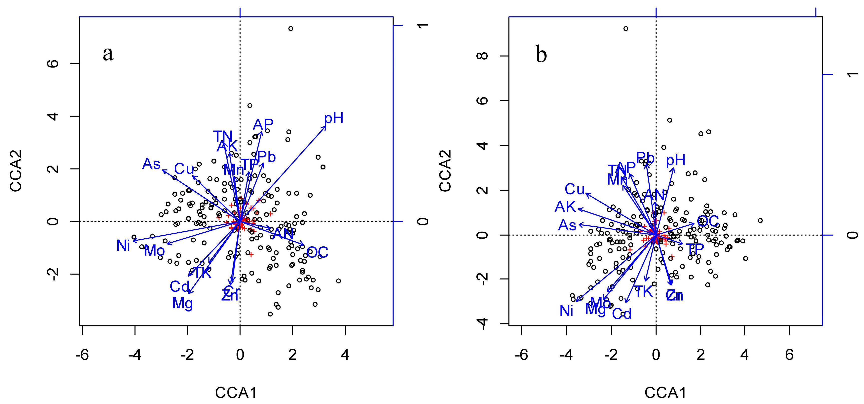
Figure 1. Canonical correspondence analysis (CCA) in two soil layers involving the upper (a) and lower layer (b). The species abundance and average values of soil nutrients in the 40 m × 40 m plots were used to test the relationship between species composition and soil elements. The species scores and site scores of the first two ordination axes are drawn in the figure. The arrow direction indicates the positive and negative correlation between the soil nutrient and ordination axes, while the length of the arrow represents the degree of correlation between certain soil nutrient variables and the community composition.
Forests 07 00159 g001
Figure 2. Boxplot of niche breadth values for 18 soil nutrients in two soil layers. The smaller the niche breadth for a given soil variable, the greater is the effect of that soil variable on the niche structure of the community.
Forests 07 00159 g002
Table 1. Pearson’s correlations between soil variables and the first two axes of canonical correspondence analysis (CCA).
Soil VariablesUpper Soil LayerLower Soil Layer
CCA1CCA2CCA1CCA2
available nitrogen−0.12−0.13−0.11−0.14
total nitrogen−0.91 ***0.07−0.91 ***0.27 ***
available potassium0.130.050.03−0.05
total potassium−0.02−0.41 ***−0.05−0.36 ***
available phosphorus−0.05−0.36 ***−0.22 **−0.44 ***
total phosphorus−0.050.120.00−0.01
organic carbon0.08−0.51 ***−0.07−0.39 ***
Cu0.07−0.26 ***0.080.10
Ni0.15 *0.19 *0.050.18 *
Cd−0.16 *−0.23 **−0.19 *−0.41 ***
As−0.34 ***0.02−0.30 ***0.03
Pb−0.100.17 *−0.070.15 *
Zn−0.21 **−0.31 ***−0.21 **−0.29 ***
Mo0.05−0.26 ***0.03−0.35 ***
Cr0.030.33 ***0.050.28 ***
Mn−0.16−0.01−0.09−0.03
Mg0.020.31 ***0.040.29 ***
pH−0.04−0.23 **−0.04−0.36 ***
* indicates p < 0.05; ** indicates p < 0.01; *** indicates p < 0.001.
Table 2. Soil variable loadings on the four principal components (PCs) in the two soil layers.
Soil VariableUpper Soil LayerLower Soil Layer
PC1PC2PC3PC4PC1PC2PC3PC4
available nitrogen−0.387−0.318−0.445−0.1220.111
total nitrogen−0.130−0.370−0.219−0.4190.164
available potassium0.191−0.306−0.3690.1400.195
total potassium−0.2290.296−0.1560.260
available phosphorus−0.379−0.119−0.1900.145−0.160
total phosphorus0.142−0.152
organic carbon0.3180.355−0.2030.202−0.267−0.308−0.238
Cu−0.252−0.3450.422−0.103−0.2220.442−0.356
Ni−0.1840.2480.315−0.2590.153−0.264
Cd−0.389−0.134−0.150−0.4150.1610.210
As−0.270−0.378−0.154−0.293−0.1650.3180.159
Pb0.113−0.2320.493−0.1030.393−0.494
Zn−0.3180.401−0.234−0.141−0.348−0.379−0.25
Mo−0.421−0.216−0.4300.1270.317
Cr−0.3110.401−0.238−0.157−0.334−0.102−0.380−0.255
Mn−0.158−0.2240.317−0.196−0.296−0.174
Mg−0.2920.1760.306−0.372
pH0.196−0.318−0.1770.149−0.384
Variance (%)21.911.310.98.920.314.110.79.1
Species (n ≥ 5)2525162324201917
Species (n ≥ 30)2423142023201716
Table 3. Relationships between species distribution and one of the first four PC axes of soil nutrients in the upper soil layer. HomP represents the homogeneous Poisson process; HomT represents the homogeneous Thomas process.
Tree SpeciesHomPHomT
PC1PC2PC3PC4PC1PC2PC3PC4
Betula platyphylla
Acer mandshuricum+
Padus racemosa
Abies nephrolepis+++
Ulmus davidiana var. japonica++
Ulmus macrocarpa+
Betula costata
Betula dahurica+
Pinus koraiensis+
Juglans mandshurica+
Sorbus pohuashanensis++
Phellodendron amurense
Tilia mandschurica+++
Ulmus laciniata++
Quercus mongolica++
Carpinus cordata++
Acer tegmentosum+++
Acer mono+
Abies holophylla+
Fraxinus mandshurica++
Sorbus alnifolia
Populus koreana
Tilia amurensis++
Syringa reticulata var. amurensis++++
Acer barbinerve++
Tilia mandschurica++
Acer ukurunduense++++
Lonicera maackii+
Euonymus macropterus+
Eleutherococcus senticosus++
Euonymus pauciflorus++
Corylus mandshurica+
Rhamnus davurica
Significant negative correlation10111192221
Significant positive correlation14123113222
Non-significant correlation910191328292930
Symbol “+” indicates significant positive correlation at the 0.05 level; Symbol “−” indicates significant negative correlation at the 0.05 level.
Table 4. Relationships between species distribution and one of the first four PC axes of soil elements in the lower soil layer. HomP represents the homogeneous Poisson process; HomT represents the homogeneous Thomas process.
Plant SpeciesHomPHomT
PC1PC2PC3PC4PC1PC2PC3PC4
Betula platyphylla++
Acer mandshuricum+++
Padus racemosa
Abies nephrolepis+
Ulmus davidiana var. japonica++
Ulmus macrocarpa+
Betula costata++
Betula dahurica+
Pinus koraiensis++
Juglans mandshurica+
Sorbus pohuashanensis
Phellodendron amurense++
Tilia mandschurica++
Ulmus laciniata+++
Quercus mongolica+
Carpinus cordata++
Acer tegmentosum++++
Acer mono+
Abies holophylla++
Fraxinus mandshurica+++
Sorbus alnifolia++
Populus koreana+++
Tilia amurensis
Syringa reticulata var. amurensis++
Acer barbinerve++
Tilia mandschurica
Acer ukurunduense+
Lonicera maackii+
Euonymus macropterus
Eleutherococcus senticosus
Euonymus pauciflorus++
Corylus mandshurica++
Rhamnus davurica
Significant negative correlation1010691111
Significant positive correlation13101171521
Non-significant correlation1013161731273031
Symbol “+” indicates significant positive correlation at the 0.05 level; Symbol “−” indicates significant negative correlation at the 0.05 level.
Table 5. Species distribution-PC associations examined by the homogeneous Thomas process in different growth groups.
Soil LayerCanopy SpeciesSubcanopy SpeciesShrub Species
23 Species5 Species5 Species
Upper
Number of species related to PC15 (3+, 2−)0 (0+, 0−)0 (0+, 0−)
Number of species related to PC23 (1+, 2−)1 (1+, 0−)0 (0+, 0−)
Number of species related to PC32 (0+, 2−)1 (1+, 0−)1 (1+, 0−)
Number of species related to PC43 (3+, 0−)1 (1+, 0−)0 (0+, 0−)
Number of species unrelated to PCs1434
Lower
Number of species related to PC12 (1+, 1−)0 (0+, 0−)0 (0+, 0−)
Number of species related to PC24 (4+, 0−)1 (0+, 1−)1 (1+, 0−)
Number of species related to PC33 (2+, 1−)0 (0+, 0−)0 (0+, 0−)
Number of species related to PC41 (1+, 0−)0 (0+, 0−)1 (0+, 1−)
Number of species unrelated to PCs1544
The first number in parentheses refers to the number of species that showed positive plant-soil relationships; the second number in parentheses is the number of species that showed negative plant-soil relationships.

