Spatial Heterogeneity of Climate Change Effects on Dominant Height of Larch Plantations in Northern and Northeastern China

Abstract

Determining the response of dominant height growth to climate change is important for understanding adaption strategies. Based on 550 permanent plots from a national forest inventory and climate data across seven provinces and three climate zones, we developed a climate-sensitive dominant height growth model under a mixed-effects model framework. The mean temperature of the wettest quarter and precipitation of the wettest month were found to be statistically significant explanatory variables that markedly improved model performance. Generally, future climate change had a positive effect on stand dominant height in northern and northeastern China, but the effect showed high spatial variability linked to local climatic conditions. The range in dominant height difference between the current climate and three future BC-RCP scenarios would change from −0.61 m to 1.75 m (−6.9% to 13.5%) during the period 2041–2060 and from −1.17 m to 3.28 m (−9.1% to 41.0%) during the period 2061–2080 across provinces. The impacts of climate change on stand dominant height decreased as stand age increased. Forests in cold and warm temperate zones had a smaller decrease in dominant height, owing to climate change, compared with those in the mid temperate zone. Overall, future climate change could impact dominant height growth in northern and northeastern China. As spatial heterogeneity of climate change affects dominant height growth, locally specific mitigation measures should be considered in forest management.

1. Introduction

As shown in IPCC reports [1], in contrast to 1986–2005, the global mean surface temperature during the period 2081–2100 is likely to increase by 0.3 °C to 4.8 °C under different climatic scenarios, and cold and hot temperature extremes will be more frequent over most land areas. As climate is a strong driver of forest growth [2], the strong effect of climate change on forests needs to be considered. However, there is no consistent understanding of the direction and magnitude of climate effects on forests. In previous studies, both positive and negative effects were reported. For instance, forest productivity can be increased by increasing atmospheric carbon dioxide, which has been called the “fertilizer effect” [3]. In contrast, extreme climate change is likely to result in huge and long-lasting decreases in forest productivity as well as in forest degradation [4].

Thought to be independent of density and thinning treatments [5,6], dominant height acts as a broadly accepted index that can be used to evaluate site quality of an even-aged, single-species stand [7]. In addition to calculating site index using a given reference age, dominant height is widely incorporated into height-diameter [8,9,10], crown ratio [11], diameter-distribution [12,13], individual tree mortality [14,15], annual survival probability [16], diameter growth [17], stand basal area growth [18,19], and stand volume growth [20,21] models. Although a climate-sensitive dominant height growth model has been developed to quantify the effects of climate change, many uncertainties and inconsistencies remain with respect to these effects. Wang et al. [22] explored the reparameterization method for Eucalyptus globulus Labill. plantations in southeastern Australia using random effects. They found that mean annual rainfall and mean daily maximum temperature in winter were significant in explaining the variation in dominant height growth. Bravo-Oviedo et al. [23] adopted the generalized algebraic difference approach for Mediterranean maritime pine (Pinus pinaster Ait.) in Spain and found drought period length, mean annual temperature, and total precipitation in autumn and winter were significant in explaining the variation in dominant height. Sharma et al. [24] reported that even though the same climate variables were found to be significant in affecting dominant height growth for different species in the same region, the directions were different. In their report, growing season total precipitation had positive effects on dominant height growth for both jack pine (Pinus banksiana Lamb.) and black spruce (Picea mariana (Mill.) B.S.P.), and growing season mean temperature can facilitate dominant height growth of black spruce and can reduce the asymptote dominant height of jack pine. Besides climate variables, soil properties have also been used as predictors in dominant height or site index models to improve empirical estimation of forest productivity [25,26,27].

Larch is one of the primary commercial plantation genera in China and comprises 6.5% of the area and 6.8% of the volume of forests across the country [28]. As climate change may induce forest degradation, deforestation, forest fire, and exotic insect pests and pathogens, and because larch is very sensitive to climate change [29], sustainable forest management for this species is facing challenges, and risk management must be considered in forest management planning. New growth models that incorporate climate variables may be the first step in providing pivotal information on how to adapt to climate change. Shen et al. [30] developed a climate-sensitive site index model for Jilin Province (mid-northeastern China). As forest response to climate change differs according to social conditions [31] and the extreme topographical conditions in northern and northeastern China, it is necessary to assess the spatial heterogeneity so as to include specific adaption measures in forest management. Until now, there are no reports assessing the spatial heterogeneity of climate change effects on the dominant height of larch plantations at a large scale in northern and northeastern China.

The two objectives of this study are as follows: (1) to develop a climate-sensitive dominant height growth model for larch plantations in northern and northeastern China, and (2) to project the effect of future climate change on dominant height growth and its spatial heterogeneity.

2. Materials and Methods

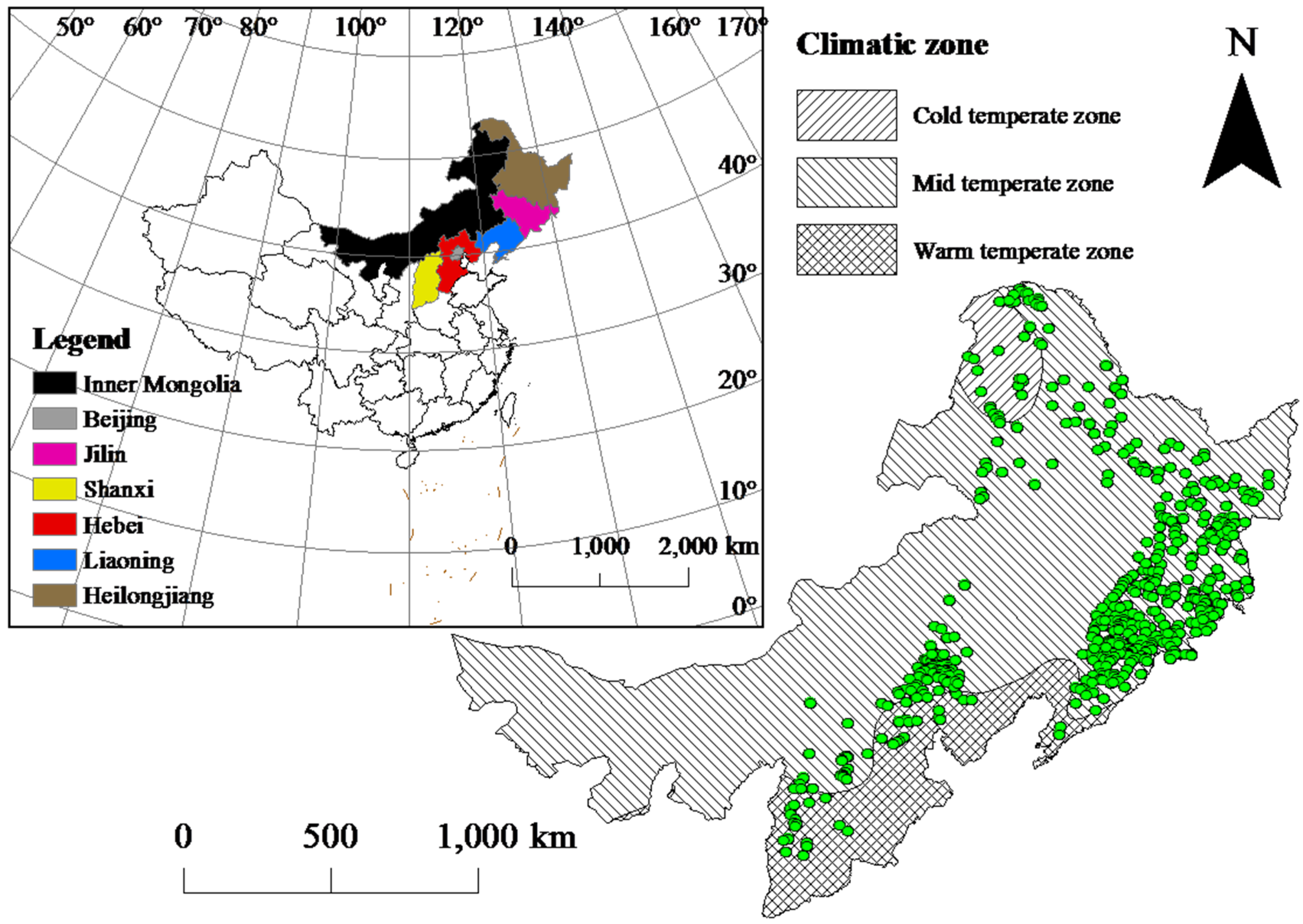
2.1. Plot Height-Age Data

A total of 550 plots obtained from the 6th, 7th, and 8th Chinese National Forestry Inventories (NFI) across seven provinces (Beijing, Hebei, Shanxi, Liaoning, Jilin, Heilongjiang, and Inner Mongolia) in northern and northeastern China were used to develop dominant height growth models. Only pure larch plantation plots were selected. All plots had three measurement records. The re-measurement intervals were 5 years for most but 4 years for a few plots. In each plot, diameter at breast height for trees larger than 5 cm was measured using a diameter tape at 1.3 m above the ground. Trees were identified to the species level with the exception of Heilongjiang, Inner Mongolia, and Shanxi, where trees were simply recorded as “Larch”. The larch species found in these plots were Larix gmelinii (Rupr.) Kuzen., Larix olgensis A. Henry, Larix kaempferi (Lamb.) Carrière, and Larix principis-rupprechtii Mayr. Height measurements were conducted in each plot for 1–3 intermediate trees using a Blume–Leiss hypsometer. Other variables measured included stand age and topography (e.g., elevation, aspect, and slope).

A height-diameter model developed by Zang et al. [32] was used to determine the total height of all trees in each plot. In addition, the height of the dominant trees was calculated as the average height of the dominant trees, which was determined for the 100 tallest trees per hectare. These data were randomly divided into two data sets: data from 495 plots (90.0%), used for model fitting, and data from the remaining 55 plots (10.0%), used for model validation. The dataset covered broad stand conditions in temperate forests, and the location of the plots is shown in Figure 1. Additional data describing the plots included in this study can be found in

Table 1. Summary of dominant height data by province.

Data	Province	Number of Plots	H (m)		Age (Years)		N (Trees·ha−1)		BA (m2·ha−1)
			Mean	SD	Mean	SD	Mean	SD	Mean	SD
Fitting data	Beijing	9	8.6	1.3	28	9.6	641	440.6	8.5	9.3
	Hebei	79	8.0	1.7	24	8.3	1141	665.8	11.8	8.9
	Heilongjiang	118	10.7	3.2	26	9.4	681	627.1	6.8	6.5
	Jilin	149	11.4	3.1	26	10.0	1113	712.0	11.6	6.7
	Liaoning	59	13.3	3.1	24	10.1	989	534.0	13.8	8.3
	Inner Mongolia	44	9.3	2.5	25	8.1	1098	861.8	11.4	8.6
	Shanxi	37	8.6	2.0	24	8.8	1196	709.8	11.4	9.2
Validation data	Beijing	1	10.9	0.5	40	5.0	1439	54.1	31.4	5.7
	Hebei	6	8.3	1.4	25	9.0	1483	726.9	15.2	8.0
	Heilongjiang	15	10.0	3.0	28	8.6	567	599.7	5.0	5.4
	Jilin	15	12.6	2.8	29	10.2	1290	535.1	15.8	6.3
	Liaoning	9	11.9	2.3	17	4.7	1445	560.4	12.7	6.2
	Inner Mongolia	6	9.1	2.8	24	9.5	893	647.3	8.1	5.3
	Shanxi	3	6.9	1.5	18	6.6	1062	532.6	6.3	4.0

H, dominant height; N, tree number per hectare; BA, basal area per hectare.

.

2.2. Climate Data

A total of 19 candidate bioclimatic variables [33] with a resolution of 1 km × 1 km over three periods: 1950–2000 (historical climate), 2041–2060, and 2061–2080 [34] for each plot were obtained from the WorldClim database [33]. The GCM model for future climate scenarios used in this study was BCC-CSM1-1 (Beijing Climate Center Climate System Model), developed by China. The 1950–2000 historical climate data were used to construct the climate-sensitive dominant height growth model, and the 2041–2060 and 2061–2080 climate data were used for projection. Three representative concentration pathways (RCPs) [35,36], RCP2.6, RCP4.5, and RCP8.5, were used to analyze the forest response to future climate change using the climate data at two time horizons, which were averaged over 20 years from 2041–2060 and 2061–2080. These pathways represent the future climate scenarios with low, medium and high concentrations of greenhouse gases and predictive radiative forcing, respectively. Therefore, a set of seven climate scenarios was obtained: current climate in the period 1950–2000, RCP2.6, RCP4.5, and RCP 8.5 in the period 2041–2060 and RCP2.6, RCP4.5, and RCP 8.5 in the period 2061–2080.

2.3. Soil Data

Soil attributes were compiled from the China Dataset of Soil Properties for Regional Land Surface Modeling [37], linked to NFI plots based on their geographic coordinates. The soil attributes had a spatial resolution of 30 × 30 arc-seconds and were derived using the soil-type linkage method and the soil polygon linkage method [38]. According to the actual depth, only 15 soil attributes (pH value, soil organic matter, total nitrogen, total phosphorus, total potassium, alkali-hydrolysable nitrogen, available phosphorus, available potassium, cation exchange capacity, exchangeable H⁺, exchangeable Ca²⁺, exchangeable Mg²⁺, exchangeable K⁺, exchangeable Na⁺, bulk density) of five layers (i.e., 0 m–0.045 m, 0.045 m–0.091 m, 0.091 m–0.166 m, 0.166 m–0.289 m, 0.289 m–0.493 m) were selected to explain the variation in dominant height growth.

2.4. Model Development

In the preliminary analysis, different growth equations [39] were assessed. The Gompertz equation performed best based on the Akaike’s information criterion (AIC), the adjusted coefficient of determination (R_a²), the mean absolute bias (MAB) and the root mean squared error (RMSE) and was used to incorporate climate variables and soil variables through re-parameterization.

$$H_{ij}=1.3+{\beta }_0\times e^{-{\beta }_1\times e^{-{\beta }_2\times Ag{e}_{ij}}}+{\epsilon }_{ij}$$

(1)

$$\mathit{AIC}=-2LL+2p$$

(2)

$${R_a}^2=1-\frac{{\displaystyle \sum _{i=1}^{n_i}{\displaystyle \sum _{j=1}^{n_{ij}}{(H_{ij}-{\widehat{H}}_{ij})}^2}}}{{\displaystyle \sum _{i=1}^{n_i}{\displaystyle \sum _{j=1}^{n_{ij}}{(H_{ij}-\overline{H})}^2}}}\times \frac{n-1}{n-p-1}$$

(3)

$$\mathit{MAB}=\frac{{\displaystyle \sum _{i=1}^{n_i}{\displaystyle \sum _{j=1}^{n_{ij}}\left|H_{ij}-{\widehat{H}}_{ij}\right|}}}{n}$$

(4)

$$\mathit{RMSE}=\sqrt{\frac{{\displaystyle \sum _{i=1}^{n_i}{\displaystyle \sum _{j=1}^{n_{ij}}{(H_{ij}-{\widehat{H}}_{ij})}^2}}}{n-p-1}}$$

(5)

where $H_{ij}$ and $Ag{e}_{ij}$ are the dominant height and stand age of the jth measurement of the ith plot, respectively; ${\epsilon }_{ij}$ is the error term; β₀, β₁, β₂ are model parameters; ${\widehat{H}}_{ij}$ is the predicted dominant height of the jth measurement in the ith plot; $\overline{H}$ is the observed mean dominant height for all data; n_i and n_ij are the total number of plots and the measurements in the ith plot, respectively; p is the number of model parameters; and LL is the log-likelihood.

To determine which factors could impact dominant height growth, three topography variables (altitude, slope, aspect), 19 climate variables, and 15 soil variables were used to express the parameters in the Gompertz function above to ensure that their influence on dominant height growth could be assessed. To avoid over-parameterization and multi-collinearity in the model, backward stepwise regression was initially used to reduce variables, and then variables with a variance inflation factor (VIF) less than five were selected. Finally, the relative weight method [40] was used to choose the final variables for expressing the parameters in the Gompertz function. Alpha = 0.05 was used to determine the form of the dominant height growth model. Details of how variables were eliminated are provided in File S1.

A mixed-effects model was adopted owing to the hierarchical structure of the data. All combinations of random parameters were tested, and the AIC criterion was used to determine the best combination [41]. The within-group residuals of the mixed effects model were analyzed for possible autocorrelation and heteroscedasticity [22], and the maximum likelihood method was used to estimate the mixed-effect model parameters [42].

The subject-specific values for a new group need to be predicted if not included in the fitting data using Equation (6) [43]

$${\widehat{U}}_i=\widehat{\Psi }{\widehat{Z}}_i^T{\left({\widehat{Z}}_i\widehat{\Psi }{\widehat{Z}}_i^T+{\widehat{R}}_i\right)}^{-1}{e}_i$$

(6)

where ${\widehat{U}}_i$ is the prediction vector for random parameters, $\widehat{\Psi }$ is the estimated variance-covariance matrix for among-group variability, ${\widehat{R}}_i$ is the estimated variance-covariance matrix for within-group variability, ${\widehat{Z}}_i$ is the partial derivatives matrix with respect to the random parameters, and $e_i$ is the residual vector determined by the difference between the observed heights and predicted heights using the mixed effects model, including only fixed effects.

The final mixed-effects model was used to project dominant height growth under different future climate scenarios. The effects of dominant height growth response to climate change were evaluated for each measurement using the difference in dominant height growth between the current (1950–2000) and future (2041–2060 and 2061–2080) climate.

In the present study, all calculations were performed using R software [44], and the nlme [45] package was used for the mixed-effects models.

3. Results

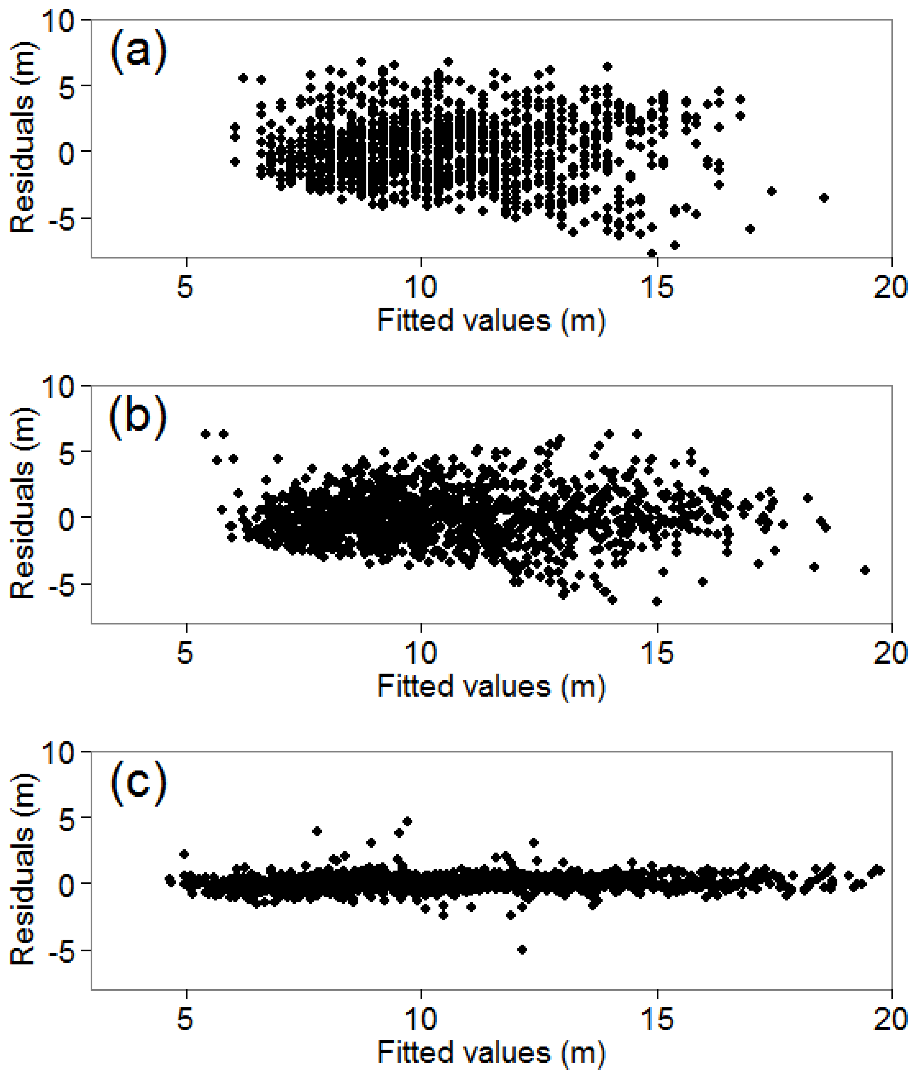
3.1. Model Development

The mean temperature of the wettest quarter (TWQ) and the precipitation of the wettest month (PWM) were found to be significant in explaining the variation in dominant height growth for larch plantations (Equation (7)). The final model (Equation (8)) with random effects was written as

$$H_{ij}=1.3+\left({\beta }_0+{\beta }_1\times PW{M}_i\right)\times e^{-{\beta }_2\times e^{-\left({\beta }_3+{\beta }_4\times TW{Q}_i\right)\times Ag{e}_{ij}}}+{\epsilon }_{ij}$$

(7)

$$H_{ij}=1.3+\left({\beta }_0+b_i+{\beta }_1\times PW{M}_i\right)\times e^{-{\beta }_2\times e^{-\left({\beta }_3+{\beta }_4\times TW{Q}_i\right)\times Ag{e}_{ij}}}+{\epsilon }_{ij}$$

(8)

with

$${\epsilon }_{ij}~N(0,{\delta }^2)$$

where TWQ_i and PWM_i represent the mean temperature of the wettest quarter and the precipitation of the wettest month of the ith plot, respectively; β₀, β₁, β₂, β₃, β₄ are fixed-effect parameters; b_i is a plot-level random parameter; and ${\delta }^2$ is the unknown scaling factor of the error within the group. All parameter estimates are listed in

Table 2. Parameter estimates and statistical criteria.

Parameter		Equation (1)	Equation (7)	Equation (8)
β0		31.2967 (9.116)	8.8033 (1.1544)	5.2349 (0.6426)
β1			0.0715 (0.008)	0.0483 (0.0038)
β2		2.0924 (0.2257)	1.7909 (0.0548)	1.9798 (0.0566)
β3		0.0209 (0.0054)	0.0162 (0.0036)	0.0372 (0.0095)
β4			0.0008 (0.0002)	0.0019 (0.0005)
δb2				2.6132
δ2				0.6894
Fitting	Ra2	0.46	0.65	0.97
	AIC	6099	5507	4247
	MAB (m)	1.92	1.47	0.37
	RMSE (m)	2.38	1.90	0.56
Validation	MAB (m)	2.29	1.69	0.34
	RMSE (m)	2.67	2.06	0.52

δ_b², variance of b_i; values in parentheses are standard deviation.

. The high variance of b_i indicated that large variation existed at the plot level; thus, other variables besides TWQ or PWM explained dominant height growth but were not included.

The statistics of the model fitting and validation are shown in Table 2. Compared to the traditional dominant height growth model (Equation (1)) (R_a² = 0.46, MAB = 1.92 m, RMSE = 2.38 m, AIC = 6099 for fitting data and MAB = 2.29 m, RMSE = 2.67 m for validation data), Equation (7) with the inclusion of climate variables (TWQ, PWM) improved the model performance (R_a² = 0.65, MAB = 1.47 m, RMSE = 1.90 m, AIC = 5507 for fitting data and MAB = 1.69 m, RMSE = 2.06 m for validation data), and the climate-sensitive dominant height growth model (Equation (8)) with random parameters vastly improved the model results (R_a² = 0.97, MAB = 0.37 m, RMSE = 0.56 m, AIC = 4247 for fitting data and MAB = 0.34 m, RMSE = 0.52 m for validation data) compared with Equations (1) and (7), and removed residual heterogeneity (Figure 2). Regardless of whether the mixed-effects model approach was used, coefficients of PWM and TWQ were positive, which implies that PWM is associated with maximum dominant height and TWQ increases the growth rate of the dominant height.

3.2. Prediction of Dominant Height Growth under Future Climate Change

As

Table 3. Predicted dominant height under future climate scenarios for all plots.

Period	Climate Scenario	TWQ				PWM				Dominant Height
		Mean	SD	ΔTWQ	ΔTWQ%	Mean	SD	ΔPWM	ΔPWM%	Mean	SD	ΔH	ΔH%
1950–2000	Current	18.5	2.32	0.00	0.0%	164.6	37.73	0.00	0.0%	10.5	3.09	0.00	0.0%
2041–2060	RCP2.6	20.8	2.34	2.32	12.5%	159.8	37.53	−4.80	−2.9%	10.6	3.16	0.10	1.0%
	RCP4.5	20.8	2.24	2.27	12.3%	189.1	45.96	24.49	14.9%	11.6	3.28	1.11	11.1%
	RCP8.5	21.8	2.24	3.23	17.5%	172.1	38.52	7.50	4.6%	11.1	3.22	0.65	6.4%
2061–2080	RCP2.6	20.4	2.29	1.84	10.0%	179.9	47.67	15.36	9.3%	11.2	3.38	0.76	7.1%
	RCP4.5	21.4	2.34	2.88	15.5%	180.6	45.92	16.04	9.8%	11.4	3.21	0.89	9.1%
	RCP8.5	22.5	2.16	3.96	21.4%	182.8	46.79	18.19	11.1%	11.6	3.42	1.13	13.3%

ΔTWQ, ΔPWM and ΔH are the mean values of each plot under future climate scenarios minus those of the current climate; ΔTWQ%, ΔPWM% and ΔH % are the values of ΔTWQ, ΔPWM and ΔH divided by the values of TWQ, PWM and H, respectively, under the current climate.

shows, compared to current climate conditions, three RCP climate scenarios show that the average difference in TWQ would range from 2.27 °C to 3.23 °C (12.3% to 17.5%) by 2041–2060 and from 1.84 °C to 3.96 °C (10.0% to 21.4%) by 2061–2080, while the average difference of PWM would range from −4.80 mm to 24.49 mm (−2.9% to 14.9%) by 2041–2060 and from 15.36 mm to 18.19 mm (9.3% to 11.1%) by 2061–2080. According to the climate-sensitive model, the dominant height change in response to future climate change, in contrast to the current climate, was calculated for all plots. The average difference in dominant height would range from −0.10 m to 1.11 m (1.0% to 11.1%) by 2041–2060 and from 0.76 m to 1.13 m (7.1% to 13.3%) by 2061–2080. The dominant height growth change in response to future climate change in different provinces is presented in Table S1. Generally, future climate change had a positive effect on dominant height growth in this region.

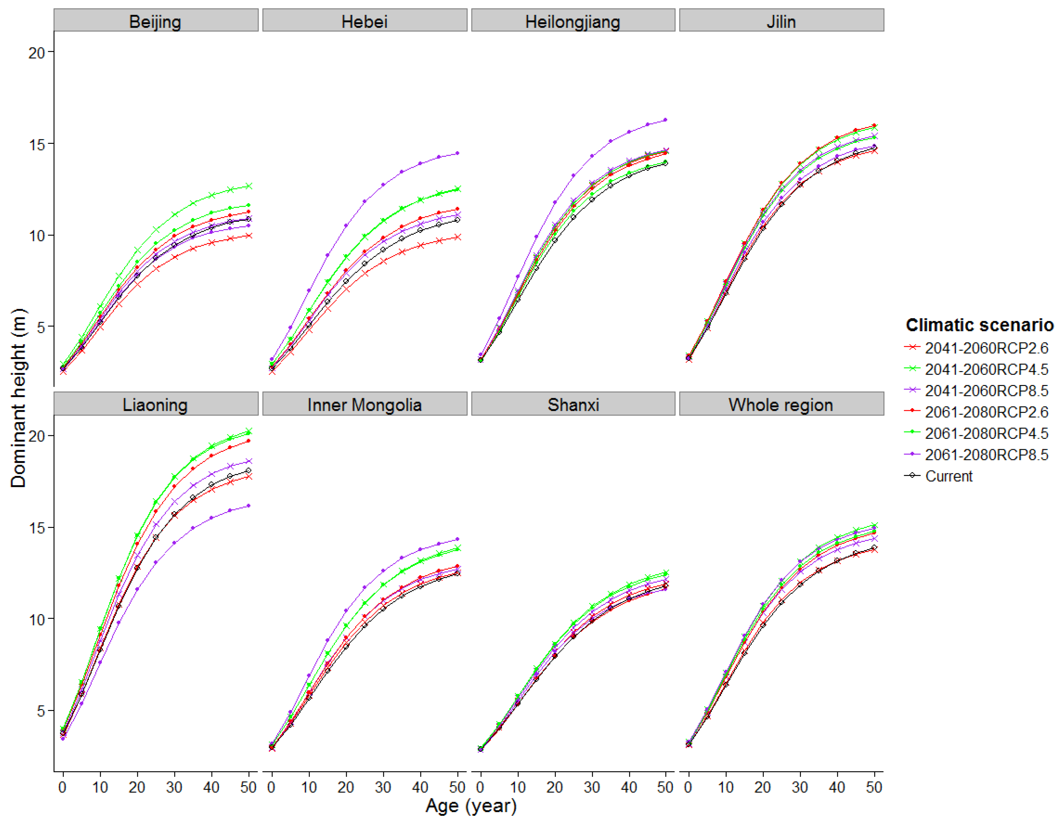
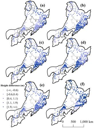
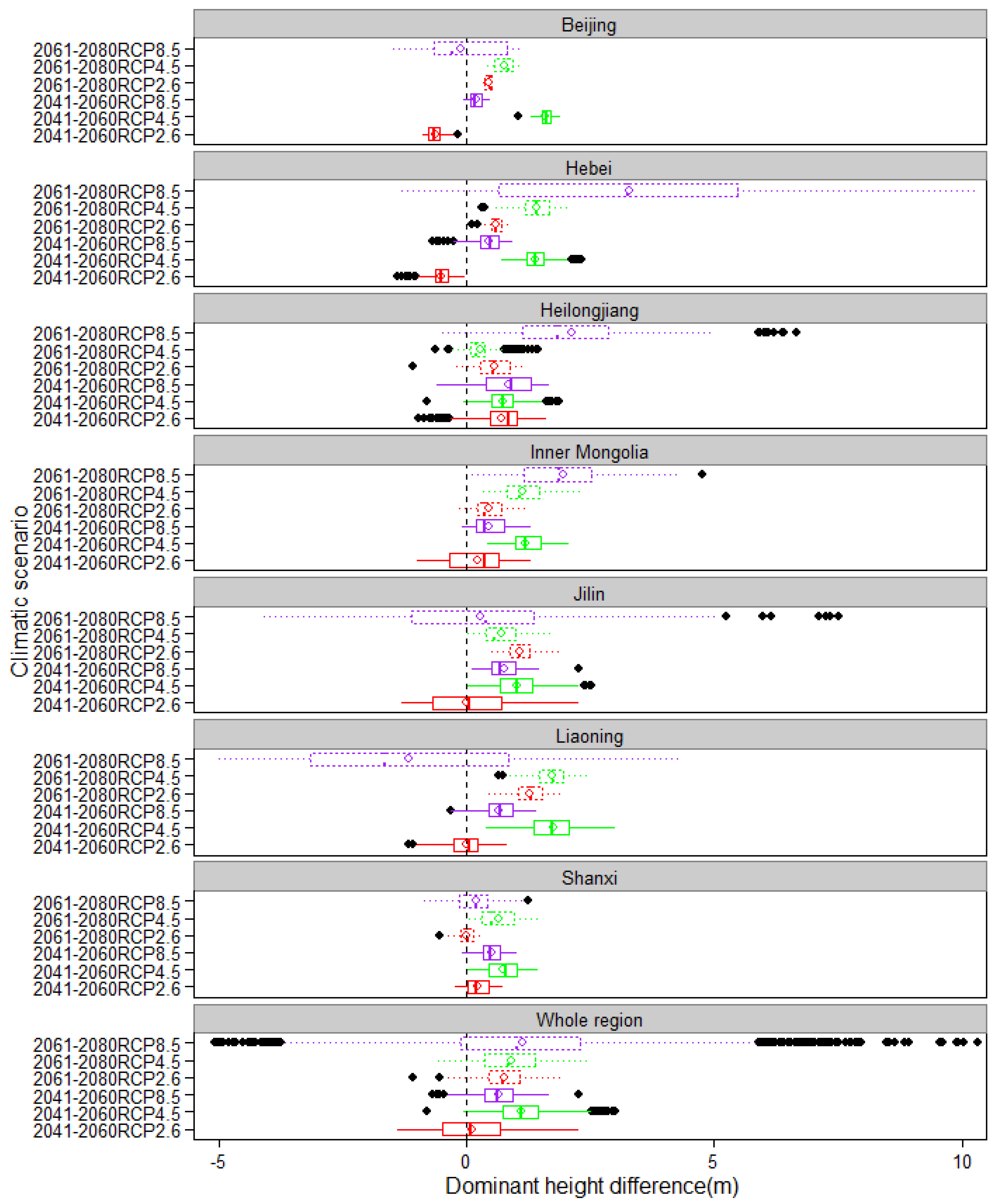
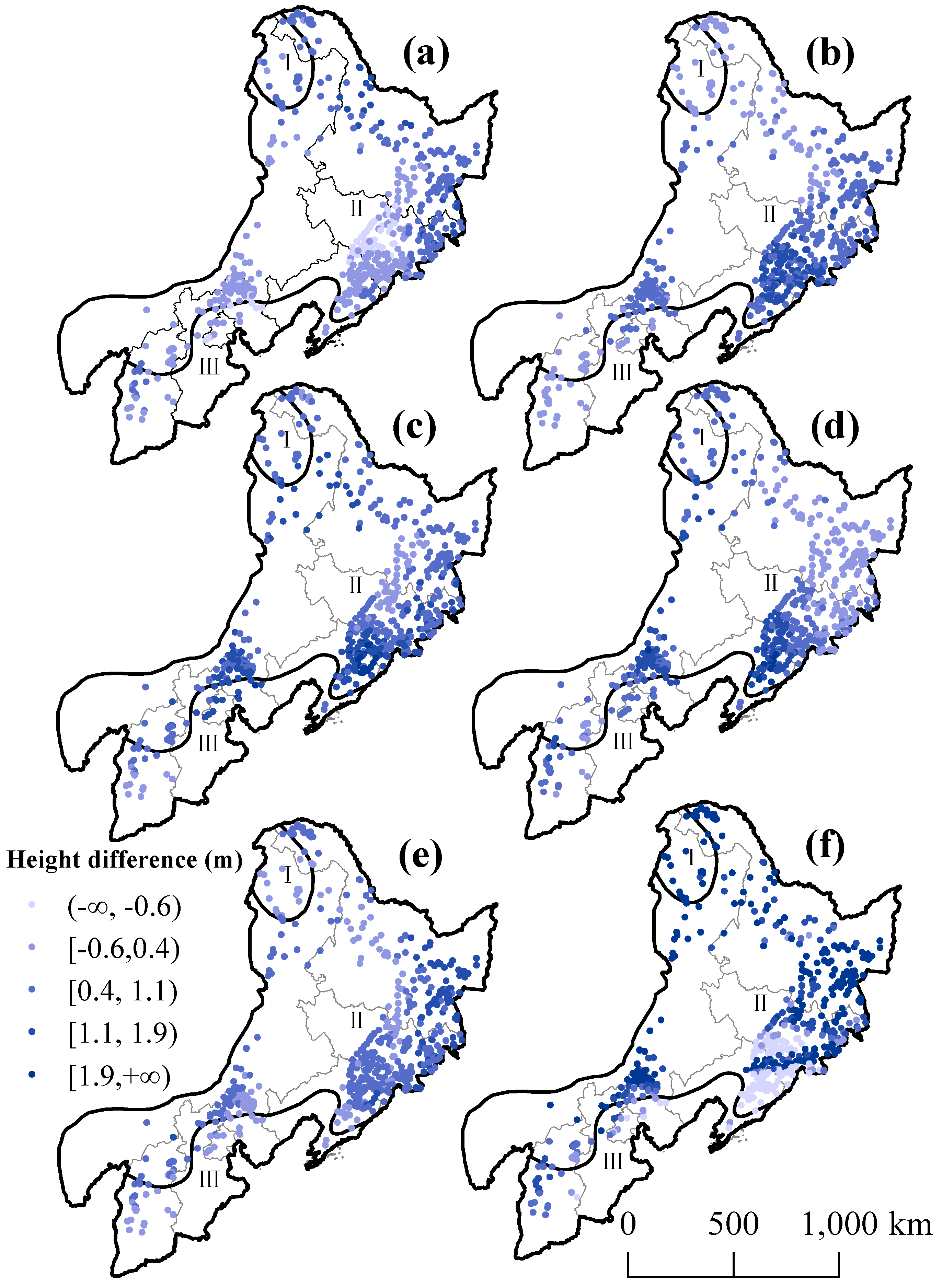
3.2.1. Growth Difference in Dominant Height across Different Provinces and Climate Zones under Future Climate Scenarios

The dominant height changes predicted under various climate scenarios did not show a consistent trend for 2041–2060 and 2061–2080, depending on the scenario and province. Although future climate change had a positive effect on dominant height growth as Table 3 shows, considerable variability existed among provinces in terms of the magnitude of the dominant height difference under different climate scenarios. Compared to the dominant height under the current climate conditions across provinces (Figure 3), we predicted that the average difference in dominant height for larch plantations would range from −0.61 m to 1.75 m (−6.9% to 13.5%) by 2041–2060 and from −1.17 m to 3.28 m (−9.1% to 41.0%) by 2061–2080. Dominant height growth in Beijing, Inner Mongolia and Shanxi was less sensitive than in Hebei, Heilongjiang, Jilin, and Liaoning. A population mean tendency was provided by the distribution of dominant height differences for the whole region (Figure 3). The mean values of the whole region under different climatic scenarios were positive, which indicated divergence in seven provinces. Furthermore, the median and mean values of the whole region showed an increased tendency following the sequence: RCP2.6 in the period 2041–2060 <RCP8.5 in the period 2041–2060 <RCP2.6 in the period 2061–2080 <RCP4.5 in the period 2061–2080 <RCP8.5 in the period 2061–2080. The sequence seems to suggest that the mean difference increases with greenhouse gas concentrations (which were represented by three climate scenarios) and time. However, the difference distribution among provinces showed a mixed circumstance, and only Hebei showed a sequence similar to the whole region. The large spatial heterogeneity of future dominant height change across the geographic scale is found in Figure 4, which is consistent with Figure 3.

To avoid a sudden change in growth process resulting from a change in climate scenarios from 2060 to 2061, we simulated the growth of dominant height using the same climate data from one of the following seven scenarios for 50 years: current, RCP2.6 in 2041–2060, RCP4.5 in 2041–2060, RCP8.0 in 2041–2060, RCP2.6 in 2061–2080, RCP4.5 in 2061–2080, RCP8.0 in 2061–2080. Figure 5 shows the dominant height profiles generated from climate-sensitive mixed-effects model (Equation (8)) using the average values of all climatic variables for larch plantations under different climate scenarios. Additionally, the dominant height profile of the whole region was also generated for comparison. It clearly showed that differences existed in the growth curve of dominant height among provinces. For example, Liaoning, Jilin and Heilongjiang had larger maximum asymptotic values than those of Beijing and Shanxi. In most cases, the values of dominant height under RCP8.5 during the period 2061–2080 were the lowest with the exception of Hebei, Heilongjiang and Inner Mongolia, and the values of dominant height under RCP4.5 during the period 2041–2060 were the highest over all provinces. In contrast, the whole region showed a population mean tendency and neglected the differences among provinces. For instance, the stand dominant height profiles of the whole region under the future climate scenarios were larger than those under the current climate, and this was inconsistent for different provinces. This is consistent with Figure 3. Generally, the increase in dominant height in the cold and warm temperate zones was smaller than that in the mid temperate zone (Figure 4).

3.2.2. Dominant Height Responses of Larch Plantations at Different Forest Stages to Climate Change

To explore whether the growth difference in dominant height varied depending on forest stage, the data were divided into four segments based on stand age: young forests (<20 years), middle-aged forests (20–30 years), pre-mature forests (30–40 years), and mature forests (≥40 years). As

Table 4. Predicted dominant height difference under future climate scenarios at different stages and under different climate scenarios.

Period	Climate Scenarios	Statistics	Young Forest	Middle-Aged Forest	Pre-Mature Forest	Mature Forest
2041–2060	RCP2.6	ΔH (m)	0.19	0.14	−0.08	0.01
		ΔH %	2.0%	1.1%	−0.6%	−0.1%
	RCP4.5	ΔH (m)	0.98	1.17	1.18	1.32
		ΔH %	11.9%	11.4%	9.9%	9.7%
	RCP8.5	ΔH (m)	0.58	0.70	0.68	0.69
		ΔH %	7.0%	6.7%	5.5%	4.8%
2061–2080	RCP2.6	ΔH (m)	0.62	0.77	0.90	0.97
		ΔH %	7.3%	7.1%	7.0%	6.5%
	RCP4.5	ΔH (m)	0.84	0.95	0.92	0.80
		ΔH %	10.4%	9.4%	7.6%	5.9%
	RCP8.5	ΔH (m)	0.94	1.27	1.34	0.80
		ΔH %	13.7%	14.4%	12.8%	7.1%

ΔH is the predicted dominant height of different climatic scenarios minus that of the current climate; ΔH% is ΔH divided by dominant height of the current climate.

shows, in most cases, the magnitude of the relative change of dominant height (ΔH%) decreased with increasing stand age with the exception of RCP8.5 during the period 2061–2080.

4. Discussion

4.1. Climate-Sensitive Dominant Height Growth Model

As sustainable forest management needs to address concerns over global climate change, new growth models will be required that incorporate climate attributes as a pivotal part of independent variables [46]. In the present study, both climate variables and edaphic variables were explored to be incorporated into a dominant height growth model, and we found TWQ and PWM were significant in explaining the variation in dominant height growth of larch plantations in northern and northeastern China. The climate-sensitive dominant height growth model improved model performance. TWQ and PWM had significant effects on parameters β₀ and β₂ in Equation (1), which represented the asymptote and growth rate of dominant height, respectively. PWM showed a positive effect on the maximum dominant height, and TWQ showed a positive effect on the rate of dominant height growth. Many studies have found that precipitation is a key factor that has often been shown to have positive effects on the growth of larch plantations [30,47]. For example, the positive effects of precipitation on stand dominant height growth were also found for jack pine and black spruce [24], and these findings are consistent with those of the present study. Similar to precipitation, a positive effect was found for the response of dominant height to temperature. Although temperature is also a key factor in forest growth [48,49], the correlation between temperature and forest growth was inconsistent in previous studies, even for larch in China. Shen et al. [30] found an opposite result to the present study, i.e., that temperature showed a negative effect on site index of Larix olgensis in Jilin, China. However, Zhang et al. [49] found a significantly positive correlation between temperature and tree-ring width for Dahurian larch in Inner Mongolia, northeastern China. For other species, Wang et al. [22] reported that temperature had a positive effect, and Sharma et al. [24] reported that an increase in temperature had positive effects on the growth of dominant height for black spruce but negative effects for jack pine in Northern Ontario, Canada. Clark et al. [50,51] found that the annual diameter increment of six species and productivity were markedly lower when temperatures increased slightly. These authors concluded this may have resulted from increased stem respiration induced by warmer temperature. In contrast to climate variables, edaphic variables were not significant in the model, and this result is consistent with the findings of some previous studies on dominant height that were reported by Fang and Bailey [52], Wang et al. [22], and Sharma et al. [24]. Although some studies [5,53,54] concluded that edaphic variables can express the variability of dominant height, we suggest this may rely on species and regions. Because CO₂ data were not available, the potential effects of changes in CO₂ and atmospheric deposition were neglected in the present study.

4.2. Projection of Dominant Height Growth under Future Climate Change

According to the climate-sensitive dominant height growth model constructed in the present study, we predicted dominant height change under different future climate scenarios and found that the average difference in dominant height of larch plantations among provinces would range from −0.61 m to 1.75 m (−6.9% to 13.5%) by 2041–2060 and from −1.17 m to 3.28 m (−9.1% to 41.0%) by 2061–2080. This implies that climate change significantly affects dominant height growth of larch plantations. In order to explore the spatial heterogeneity, we analyzed the sensitivity among provinces with respect to dominant height difference between future climate scenarios and current climate (Figure 3), and between the provinces and the whole region. We found that dominant height growth in Beijing, Inner Mongolia, and Shanxi was less sensitive than in Hebei, Heilongjiang, Jilin, and Liaoning, and forests in cold and warm temperate zones had lower sensitivity to climate change than those in the mid temperate zone. Furthermore, a significant trend was found, i.e., the change in dominant height decreased with an increase in forest age. The dominant height difference for each plot was also investigated and ranged from −5.09 m to 10.31 m (−39.7% to 121.9%), which was caused by the extreme climate change under the predicted future climate scenarios. The values of the climatic variables under the future climate scenarios were projected based on underlying scenario assumptions, and the dominant height was calculated using a height-diameter model [32]; thus, uncertainty exists in the model predictions, which need to be highlighted clearly to the model user. In addition, the prediction risk arising from the uncertainty using a future climate dataset based on a small numbers of climate variables may cause large variation. Uncertainty in the model prediction of dominant height/site index under climate change was also observed in previous studies. Shen et al. [30] found that the average site index of Larix olgensis A. Henry ranged from 0.3 m (2.2%) to −0.8 m (−5.9%) by 2050 and from 0.5 m (3.7%) to −1.6 m (−11.8%) by 2070 in Jilin province, China. Albert and Schmidt [55] predicted a change in site index for the period 2041–2050 that varied from −1.19 m to −2.87 m (−4.4% to −10.5%) with decreasing precipitation and from −0.24 m to 2.05 m (−0.8% to 7.7%) with increasing temperature. Bravo-Oviedo et al. [56] found that the change in site index prediction of Spanish Pinus pinaster Ait. fluctuated greatly between −30% and 12.5%. Weiskittel et al. [57] predicted that the predominant trend from 2000 to 2090 was a 0–5 m (0%–30%) increase in the average site index across forests of the western part of the United States. When using model outputs from climate-sensitive growth models, caution should be taken because of the uncertainty arising from the different climate scenarios, model errors, and tree species.

4.3. Management Implications for Larch Plantations

Because of the uncertainties discussed above, it is difficult to accurately quantify how climate change may affect forest management. However, climate-sensitive forest growth models represent an important step towards providing relevant information for making adaptive management decisions associated with future climatic conditions. In order to balance timber supply and demand and to guarantee national timber security, the National Strategic Timber Reserve Plan from 2015 to 2020 was issued by the Chinese government, and larch was identified as a main tree genera. To achieve this goal, we developed a climate-sensitive dominant height growth model that can be used to quantify climate-related site quality and provide information on spatial variation of how climate change affects dominant height growth over time. In terms of the projections made in the present study, young forests were more sensitive to climate change than old forests, and managers may need to pay more attention to young forests. As both increases and decreases were found, rotation age may need to be adjusted according to the changes in growth rate. Moreover, more careful adaptive measures should be implemented in larch plantations in Hebei, Heilongjiang, Jilin, and Liaoning, which are more sensitive to climate change than those in Beijing, Inner Mongolia, and Shanxi. Our results also suggested the need for locally specific adaptation measures, owing to the large effects of spatial heterogeneity associated with climate change. Additionally, because of uncertainties related to climate scenarios and model errors, model users should be careful if their findings differ significantly from their experiences. Furthermore, future validation should be considered, and risk management should be implemented in forest management.

References

1. IPCC. Climate change 2014: Synthesis report. In Contribution of Working Groups I, II and III to the Fifth Assessment Report of the Intergovernmental Panel on Climate Change; Core Writing Team, Pachauri, R.K., Meyer, L.A., Eds.; IPCC: Geneva, Switzerland, 2014; p. 151. [Google Scholar]
2. Toledo, M.; Poorter, L.; Peña-Claros, M.; Alarcón, A.; Balcázar, J.; Leaño, C.; Licona, J.C.; Llanque, O.; Vroomans, V.; Zuidema, P.; et al. Climate is a stronger driver of tree and forest growth rates than soil and disturbance. J. Ecol. 2011, 99, 254–264. [Google Scholar] [CrossRef]
3. Nemani, R.R.; Keeling, C.D.; Hashimoto, H.; Jolly, W.M.; Piper, S.C.; Tucker, C.J.; Myneni, R.B.; Running, S.W. Climate driven increases in global terrestrial net primary production from 1982 to 1999. Science 2003, 300, 1560–1563. [Google Scholar] [CrossRef] [PubMed]
4. Khaine, I.; Woo, S.Y. An overview of interrelationship between climate change and forests. For. Sci. Technol. 2015, 11, 11–18. [Google Scholar] [CrossRef]
5. Bošeľa, M.; Máliš, F.; Kulla, L.; Šebeň, V.; Deckmyn, G. Ecologically based height growth model and derived raster maps of Norway spruce site index in the Western Carpathians. Eur. J. For. Res. 2013, 132, 691–705. [Google Scholar] [CrossRef]
6. Sharma, R.P.; Brunner, A.; Eid, T.; Øyen, B.-H. Modelling dominant height growth from national forest inventory individual tree data with short time series and large age errors. For. Ecol. Manag. 2011, 262, 2162–2175. [Google Scholar] [CrossRef]
7. Skovsgaard, J.P.; Vanclay, J.K. Forest site productivity: A review of the evolution of dendrometric concepts for even-aged stands. Forestry 2008, 81, 13–31. [Google Scholar] [CrossRef]
8. Calama, R.; Montero, G. Interregional nonlinear height-diameter model with random coefficients for stone pine in Spain. Can. J. For. Res. 2004, 34, 150–163. [Google Scholar] [CrossRef]
9. Gómez-García, E.; Fonseca, T.F.; Crecente-Campo, F.; Almeida, L.R.; Diéguez-Aranda, U.; Huang, S.; Marques, C.P. Height-diameter models for maritime pine in Portugal: A comparison of basic, generalized and mixed-effects models. iForest 2015, 9, 72–78. [Google Scholar] [CrossRef]
10. Paulo, J.A.; Tomé, J.; Tomé, M. Nonlinear fixed and random generalized height-diameter models for Portuguese cork oak stands. Ann. For. Sci. 2011, 68, 295–309. [Google Scholar] [CrossRef]
11. Soares, P.; Tomé, M. A tree crown ratio prediction equation for eucalypt plantations. Ann. For. Sci. 2001, 58, 193–202. [Google Scholar] [CrossRef]
12. Cao, Q.V. Predicting parameters of a Weibull function for modeling diameter distribution. For. Sci. 2004, 50, 682–685. [Google Scholar]
13. Newton, P.F.; Lei, Y.; Zhang, S.Y. Stand-level diameter distribution yield model for black spruce plantations. For. Ecol. Manag. 2005, 209, 181–192. [Google Scholar] [CrossRef]
14. Adame, P.; del Río, M.; Cañellas, I. Modeling individual-tree mortality in Pyrenean oak (Quercus pyrenaica Willd.) stands. Ann. For. Sci. 2010, 67, 810. [Google Scholar] [CrossRef]
15. Crecente-Campo, F.; Marshall, P.; Rodríguez-Soalleiro, R. Modeling non-catastrophic individual-tree mortality for Pinus radiata plantations in northwestern Spain. For. Ecol. Manag. 2009, 257, 1542–1550. [Google Scholar] [CrossRef]
16. Crecente-Campo, F.; Marshall, P.; Rodríguez-Soalleiro, R. Modelling annual individual-tree growth and mortality of Scots pine with data obtained at irregular measurement intervals and containing missing observations. For. Ecol. Manag. 2010, 260, 1965–1974. [Google Scholar] [CrossRef]
17. De-Miguel, S.; Guzmán, G.; Pukkala, T. A comparison of fixed- and mixed-effects modeling in tree growth and yield prediction of an indigenous neotropical species (Centrolobium tomentosum) in a plantation system. For. Ecol. Manag. 2013, 291, 249–258. [Google Scholar] [CrossRef]
18. Pienaar, L.V.; Shiver, B.D. Basal area prediction and projection equations for pine plantations. For. Sci. 1986, 32, 626–633. [Google Scholar]
19. Zhao, L.; Li, C. Stand basal area model for Cunninghamia lanceolata (Lamb.) Hook. plantations based on a multilevel nonlinear mixed-effect model across south-eastern China. South For. 2013, 75, 41–50. [Google Scholar]
20. Fang, Z.; Bailey, R.L.; Shiver, B.D. A multivariate simultaneous prediction system for stand growth and yield with fixed and random effects. For. Sci 2001, 47, 550–562. [Google Scholar]
21. Hall, D.B.; Clutter, M. Multivariate multilevel nonlinear mixed effects models for timber yield predictions. Biometrics 2004, 60, 16–24. [Google Scholar] [CrossRef] [PubMed]
22. Wang, Y.; LeMay, V.M.; Baker, T.G. Modelling and prediction of dominant height and site index of Eucalyptus globulus plantations using a nonlinear mixed-effects model approach. Can. J. For. Res. 2007, 37, 1390–1403. [Google Scholar] [CrossRef]
23. Bravo-Oviedo, A.; Tomé, M.; Bravo, F.; Montero, G.; del Río, M. Dominant height growth equations including site attributes in the generalized algebraic difference approach. Can. J. For. Res. 2008, 38, 2348–2358. [Google Scholar] [CrossRef]
24. Sharma, M.; Subedi, N.; Ter-Mikaelian, M.; Parton, J. Modeling climatic effects on stand height/site index of plantation-grown jack pine and black spruce trees. For. Sci. 2015, 61, 25–34. [Google Scholar] [CrossRef]
25. Aertsen, W.; Kint, V.; De Vos, B.; Deckers, J.; Van Orshoven, J.; Muys, B. Predicting forest site productivity in temperate lowland from forest floor, soil and litterfall characteristics using boosted regression trees. Plant Soil 2012, 354, 157–172. [Google Scholar] [CrossRef]
26. Jiang, H.; Radtke, P.J.; Weiskittel, A.R.; Coulston, J.W.; Guertin, P.J. Climate- and soil-based models of site productivity in eastern US tree species. Can. J. For. Res. 2015, 45, 325–342. [Google Scholar] [CrossRef]
27. McKenney, D.W.; Pedlar, J.H. Spatial models of site index based on climate and soil properties for two boreal tree species in Ontario, Canada. For. Ecol. Manag. 2003, 175, 497–507. [Google Scholar] [CrossRef]
28. State Forestry Administration, The People’s Republic of China. National Forest Resources Statistics (2009–2013); State Forestry Administration: Beijing, China, 2014; p. 233. (In Chinese) [Google Scholar]
29. Cook, E.R.; Kairiukstis, L.A. Methods of Dendrochronology: Applications in the Environmental Sciences; Kluwer Academic Publishers: Dordrecht, The Netherlands, 1989; pp. 25–26. [Google Scholar]
30. Shen, C.; Lei, X.; Liu, H.; Wang, L.; Liang, W. Potential impacts of regional climate change on site productivity of Larix olgensis plantations in northeast China. iForest 2015, 8, 642–651. [Google Scholar] [CrossRef]
31. Parks, C.G.; Bernier, P. Adaptation of forests and forest management to changing climate with emphasis on forest health: A review of science, policies and practices. For. Ecol. Manag. 2010, 259, 657–659. [Google Scholar] [CrossRef]
32. Zang, H.; Lei, X.; Zeng, W. Height-diameter equations for larch plantations in northern and northeastern China: A comparison of the mixed effects, quantile regression and generalized additive models. Forestry 2016. [Google Scholar] [CrossRef]
33. WorldClim-Global Climate Data. Available online: http://www.worldclim.org (accessed on 3 July 2016).
34. Hijmans, R.J.; Cameron, S.E.; Parra, J.L.; Jones, P.G.; Jarvis, A. Very high resolution interpolated climate surfaces for global land areas. Int. J. Climatol. 2005, 25, 1965–1978. [Google Scholar] [CrossRef]
35. Moss, R.; Babiker, M.; Brinkman, S.; Calvo, E.; Carter, T.; Edmonds, J.; Elgizouli, I.; Emori, S.; Erda, L.; Hibbard, K.; et al. Towards New Scenarios for Analysis of Emissions, Climate Change, Impacts, and Response Strategies; Intergovernmental Panel on Climate Change: Noordwijkerhout, The Netherlands, 2008; p. 14. [Google Scholar]
36. Van Vuuren, D.P.; Edmonds, J.; Kainuma, M.; Riahi, K.; Thomson, A.; Hibbard, K.; Hurtt, G.C.; Kram, T.; Krey, V.; Lamarque, J.F.; et al. The representative concentration pathways: An overview. Clim. Chang. 2011, 109, 5–31. [Google Scholar] [CrossRef]
37. Shangguan, W.; Dai, Y.; Liu, B.; Zhu, A.; Duan, Q.; Wu, L.; Ji, D.; Ye, A.; Yuan, H.; Zhang, Q.; et al. A China dataset of soil properties for land surface modeling. J. Adv. Model. Earth Syst. 2013, 5, 212–224. [Google Scholar] [CrossRef]
38. Shangguan, W.; Dai, Y.; Liu, B.; Ye, A.; Yuan, H. A soil particle-size distribution dataset for regional land and climate modeling in China. Geoderma 2012, 171–172, 85–91. [Google Scholar] [CrossRef]
39. Zeide, B. Analysis of growth equations. For. Sci. 1993, 39, 594–616. [Google Scholar]
40. Johnson, J.W. A heuristic method for estimating the relative weight of predictor variables in multiple regression. Multivar. Behav. Res. 2000, 35, 1–19. [Google Scholar] [CrossRef] [PubMed]
41. Yang, Y.; Huang, S.; Meng, S.X.; Trincado, G.; VanderSchaaf, C.L. A multilevel individual tree basal area increment model for aspen in boreal mixed wood stands. Can. J. For. Res. 2009, 39, 2203–2214. [Google Scholar] [CrossRef]
42. Lindstrom, M.J.; Bates, D.M. Nonlinear mixed effects models for repeated measures data. Biometrics 1990, 46, 673–687. [Google Scholar] [CrossRef] [PubMed]
43. Vonesh, E.F.; Chinchilli, V.M. Linear and Nonlinear Models for the Analysis of Repeated Measurements; Marcel Dekker: New York, NY, USA, 1997; p. 343. [Google Scholar]
44. R Development Core Team. R: A Language and Environment for Statistical Computing; R Foundation for Statistical Computing: Vienna, Austria, 2015; Available online: http://www.r-project.org (accessed on 12 January 2016).
45. Pinheiro, J.C.; Bates, D.M.; Debroy, S.; Sarkar, D.; EISPACK authors; R Core Team. Nlme: Linear and Nonlinear Mixed Effects Models; R Package Version 3.1–102; Available online: http://www.cran.r-project.org/web/packages/nlme/nlme.pdf (accessed on 12 January 2016).
46. Nothdurft, A.; Wolf, T.; Ringeler, A.; Bohner, J.; Saborowski, J. Spatio-temporal prediction of site index based on forest inventories and climate change scenarios. For. Ecol. Manag. 2012, 279, 97–111. [Google Scholar] [CrossRef]
47. Dulamsuren, C.; Hauck, M.; Bader, M.; Osokhjarga, D.; Oyungere, S.; Nyambayar, S.; Runge, M.; Leuschner, C. Water relations and photosynthetic performance in Larix sibirica growing in the forest-steppe ecotone of northern Mongolia. Tree Physiol. 2009, 29, 99–110. [Google Scholar] [CrossRef] [PubMed]
48. Panyushkina, I.P.; Ovtchinnikov, D.V.; Adamenko, M.F. Mixed response of decadal variability in larch tree-ring chronologies from upper tree-lines of the Russian Altai. Tree-Ring Res. 2005, 61, 33–42. [Google Scholar] [CrossRef]
49. Zhang, X.; He, X.; Li, J.; Davi, N.; Chen, Z.; Cui, M.; Chen, W.; Li, N. Temperature reconstruction (1750–2008) from Dahurian larch tree-rings in an area subject to permafrost in Inner Mongolia, Northeast China. Clim. Res. 2011, 47, 151–159. [Google Scholar] [CrossRef]
50. Clark, D.A.; Piper, S.C.; Keeling, C.D.; Clark, D.B. Tropical rain forest tree growth and atmospheric carbon dynamics linked to inter-annual temperature variation during 1984–2000. Proc. Natl. Acad. Sci. USA 2003, 100, 5852–5857. [Google Scholar] [CrossRef] [PubMed]
51. Clark, D.B.; Clark, D.B.; Oberbauer, S.F. Annual wood production in a tropical rain forest in NE Costa Rica linked to climatic variation but not to increasing CO2. Glob. Chang. Biol. 2010, 16, 747–759. [Google Scholar] [CrossRef]
52. Fang, Z.; Bailey, R.L. Nonlinear mixed effects modeling for slash pine dominant height growth following intensive silvicultural treatments. For. Sci. 2001, 47, 287–300. [Google Scholar]
53. Bergès, L.; Balandier, P. Revisiting the use of soil water budget assessment to predict site productivity of sessile oak (Quercus petraea Liebl.) in the perspective of climate change. Eur. J. For. Res. 2010, 129, 199–208. [Google Scholar] [CrossRef]
54. Seynave, I.; Gégout, J.-C.; Hervé, J.-C.; Dhôte, J.-F.; Drapier, J.; Bruno, É.; Dumé, G. Picea abies site index prediction by environmental factors and understorey vegetation: A two-scale approach based on survey databases. Can. J. For. Res. 2005, 35, 1669–1678. [Google Scholar] [CrossRef]
55. Albert, M.; Schmidt, M. Climatic-sensitive modeling of site-productivity relationships for Norway spruce (Picea abies (L.) Karst.) and common beech (Fagus sylvatica L.). For. Ecol. Manag. 2010, 259, 739–749. [Google Scholar] [CrossRef]
56. Bravo-Oviedo, A.; Gallardo-Andrés, C.; del Río, M.; Montero, G. Regional changes of Pinus pinaster site index in Spain using a climate-based dominant height model. Can. J. For. Res. 2010, 40, 2036–2048. [Google Scholar] [CrossRef]
57. Weiskittel, A.R.; Crookston, N.L.; Radtke, P.J. Linking climate, gross primary productivity and site index across forests of the western United States. Can. J. For. Res. 2011, 41, 1710–1721. [Google Scholar] [CrossRef]
Figure 1. The distribution of plots. Latitude and longitude ranged from 34°34′ N to 53°33′ N and 97°12′ E to 135°05′ E, respectively; the geographic coordinate system of this map was GCS_Clarke_1866.
Forests 07 00151 g001
Figure 2. Residuals for dominant height growth models, (a) Equation (1); (b) Equation (7); (c) Equation (8).
Forests 07 00151 g002
Figure 3. Boxplot of the predicted dominant height difference between different climate scenarios and current climate for seven provinces and the whole region; the hollow circles in each bar indicate the average values; the dashed vertical lines show zero lines (no dominant height difference).
Forests 07 00151 g003
Figure 4. The distribution of the differences between the predicted dominant height of different climate scenarios and the current predicted dominant height, (a) RCP2.6 during the period 2041–2060; (b) RCP2.6 during the period 2061–2080; (c) RCP4.5 during the period 2041–2060; (d) RCP4.5 during the period 2061–2080; (e) RCP8.5 during the period 2041–2060; (f) RCP8.5 during the period 2061–2080. The bold line shows the climatic zones: I for the cold temperate zone, II for the mid temperate zone and III for the warm temperate zone; the geographic coordinate system of these maps is GCS_Clarke_1866.
Forests 07 00151 g004
Figure 5. The dominant height profiles generated using the average values of all climate variables in different provinces and under different climatic scenarios.
Forests 07 00151 g005