Developing Two Additive Biomass Equations for Three Coniferous Plantation Species in Northeast China

Abstract

Accurate quantification of tree biomass is critical and essential for calculating carbon storage, as well as for studying climate change, forest health, forest productivity, nutrient cycling, etc. Tree biomass is typically estimated using statistical models. In this study, a total of 289 trees were harvested and measured for stem, root, branch, and foliage biomass from three coniferous plantation species in northeastern P.R. China. We developed two additive systems of biomass equations based on tree diameter (D) only and both tree diameter (D) and height (H). For each system, likelihood analysis was used to verify the error structures of power functions in order to determine if logarithmic transformation should be applied on both sides of biomass equations. The model coefficients were simultaneously estimated using seemingly unrelated regression (SUR). The results indicated that stem biomass had the largest relative contribution to total biomass, while foliage biomass had the smallest relative proportion for the three species. The root to shoot ratio averaged 0.27 for Korean pine, 0.25 for larch, and 0.23 for Mongolian pine. The two additive biomass systems obtained good model fitting and prediction performance, of which the model R_a² > 0.80, and the percent mean absolute bias (MAB%), was <17%. The second additive system (D and H) had a relatively greater R_a² and smaller root mean square error (RMSE). The model coefficient for the predictor H was statistically significant in eight of the twelve models, depending on tree species and biomass component. Adding tree height into the system of biomass equations can marginally improve model fitting and performance, especially for total, aboveground, and stem biomass. The two additive systems developed in this study can be applied to estimate individual tree biomass of three coniferous plantation species in the Chinese National Forest Inventory.

1. Introduction

Tree biomass is the foundation of forest ecosystems, and has been subject to research for over a century. In recent years, estimating tree total and component biomass has been greatly increased (e.g., [1,2,3,4]) because they are needed when predicting net primary production (NPP) for different stands or regions, and estimating total carbon and fluxes in forest ecosystems [5,6,7,8].

Total tree biomass is commonly divided into different components according to their physiological functions such as stems, roots, branches, and foliage. Although directly measuring the actual weight of each component is undoubtedly the most accurate method, it is destructive, time consuming, and costly. Thus, using allometric equations to develop biomass models is considered a better and more feasible approach to estimating tree-level biomass [9,10,11]. Over the last few decades, more than 2600 biomass models have been developed for more than 100 species around the world [12,13,14,15,16,17], especially for the aboveground biomass. Belowground biomass is an important component of forest biomass that demands more investigation and study. However, this component is not tracked in many forest inventories, because extracting tree roots is expensive and time consuming, and the techniques for measuring root biomass are poorly developed compared to stem, branch and foliage biomass [11,18]. Until now, only few models have been made available for tree belowground or root biomass. For these biomass models published in the literature, tree diameter at breast height (D) is the most commonly used and reliable predictor for total, sub-total, and components biomass [11,19,20,21,22,23]. Although other tree variables have been investigated as potential predictors for tree biomass models, tree total height is considered the best, in addition to tree diameter, to significantly improve model fitting and performance [24,25,26,27,28].

The allometric equation Y = a × X^b is a mathematical function commonly used for tree biomass modeling. In practice, logarithmic transformation is routinely used to fit the allometric equation using ordinary least squares regression [14,29,30]. However, some researchers suggest that data analysis and modeling should be performed on the original data of measurement via nonlinear regression [10,27]. The choice between linear regression on log-transformed data (LR) or nonlinear regression on original data (NLR) depends on the model error structure. NLR fits the original data by nonlinear least squares assuming an additive error structure for the allometric equation, whereas LR fits the log-transformed data assuming the underlying power function with a multiplicative error structure. To facilitate the objective determination on the model error structures, Bi et al. [10] compared the predictive performance of the two model specifications for a system of additive biomass equations using the ratio of their mean squared errors. Xiao et al. [31] and Ballantyne [32] outlined the approach of likelihood analysis to evaluating and comparing model error structures, which was recently used for tree biomass [30,33]. Compared with the MSE ratio approach, the likelihood analysis is considered to be consistent with core statistical principles, and more suitable in determining model error structures [32].

To date, biomass equations for estimating tree total, sub-total, and component biomass can be classified into non-additive and additive in nature. Non-additive biomass equations fit the biomass data of total, sub-total and components separately. Consequently, the sum of model predictions from component biomass models may not be equal to the model prediction from the total biomass model. In contrast, additive biomass equations fit the biomass data of total, sub-total and components simultaneously to account for the inherent correlations among biomass components measured on the same sample trees. Thus, the sum of biomass predictions from the component biomass equations is equal to the biomass prediction from the total or sub-total equation [34,35]. To achieve the additivity for a system of biomass equations, different model parameter estimation methods have been suggested for both linear and nonlinear biomass models [10,34,35,36]. In particular, seemingly unrelated regression (SUR) and nonlinear seemingly unrelated regression (NSUR) are more general and flexible, and have become more popular as the parameter estimation method for linear and nonlinear biomass equations [37,38,39,40,41].

Past research has indicated that the origin of forest stands may influence the biomass estimation [26,42,43,44]. Generally, if a tree species exists in both plantation and natural forests, the biomass models should be developed separately for each forest origin. In the forest regions of northeastern China, Korean pine (Pinus koraiensis Sieb. et Zucc.), larch (Larix gmelinii (Rupr.) Kuzen.) and Mongolian pine (Pinus sylvestris var. mongolica Litv.) are three major species growing in plantation forests. To date, Wang [11] and Dong et al. [33] developed biomass equations for Korean pine and larch in northeastern China. However, Wang’s [11] biomass data were collected from a limited forest region with a relatively small sample size for each species. The biomass data of Dong et al. [33] came from natural forest stands. For Mongolian pine, there was very limited information available on aboveground and belowground or root biomass. Thus, the objectives of this study were: (1) to analyze the biomass partitioning for the three species; (2) to examine which model error structure is more suitable for the allometric biomass relationships; (3) to develop two additive systems of biomass equations for the three species; and (4) to validate the performance of the biomass models through the jackknifing technique across the classes of tree diameter.

2. Materials and Methods

2.1. Site Description

The study area covered the Zhangguangcai Mountains (about 126°31′ E–131°44′ E, 43°35′ N–46°09′ N) and Xiaoxing’an Mountains (about 127°42′ E–130°14′ E, 46°28′ N–49°21′ N), located in Heilongjiang Province, China (Figure 1). A total of 83 plots were selected, and each plot was 30 × 30 m or 20 × 30 m in size. For these plots, there were three forest types (i.e., Korean pine, larch, and Mongolian pine pure plantations.) distributed in various site conditions. The characteristics of these forest types and the geographical location in this study were described in

Table 1. Characteristics of forest types from which the sample trees were selected.

Forest Types	Plots	Density (Trees·ha−1)	Age (Years)	Dq (cm)	Slope (°)	Altitude (m)
Korean pine plantation	36	650–1650	16–48	12.3–21.5	0–12	194–467
Larch plantation	17	700–1850	12–53	15.7–29.6	0–10	120–385
Mongolian pine plantation	30	452–1662	12–46	6.3–29.2	2–20	124–376

Note: Dq represents the quadratic mean diameter at breast height (1.3 m above ground level).

and Figure 1.

2.2. Destructive Tree Sampling

The data used in this study were selected from a large data set of tree biomass. The tree species included Korean pine (Pinus koraiensis Sieb. et Zucc.), Larch (Larix gmelinii (Rupr.) Kuzen.), and Mongolian pine (Pinus sylvestris var. mongolica Litv.) in the pure plantations of northeastern P.R. China. The sample plots were established over a five-year period from 2009 to 2013. For each of the 83 plots, at least one tree(s) was carefully selected from each of the dominant, intermediate and suppressed trees. Thus, a total of 114 Korean pine trees, 90 larch trees, and 85 Mongolian pine trees were destructively sampled as follows: the stems of the sampled trees were cut at the ground and the total height (H) and diameter at the breast height (D) were immediately measured and recorded. Then, the stems were cut into 1 m sections and each section was weighed and recorded. At the end of each stem section, a 2–3 cm thick disc was cut and weighed. The live crown (from the first dead branch to base of the terminal bud) was equally marked into three layers (i.e., top, middle, and bottom). All live branches in each crown layer were cut and weighed. Then, in each crown layer, 3–5 branches were cut and the branch and foliage were separated and weighed, respectively. The branches and foliage were then sampled (about 50–100 g), weighed and taken to the laboratory for moisture content determination. The entire roots of large trees were excavated using a chain (i.e., lifting equipment) and manually digging combination approach, and the roots of small trees were only dug manually. Because of the heavy workload and difficulty in excavating the roots, the fine roots < 5 mm were not included. All roots of the sampled trees were divided into three categories: large roots (diameter ≥ 5 cm), medium roots (2–5 cm), and small roots (diameter < 2 cm). Each root was sampled (about 100–200 g), weighed, and taken to the lab for moisture content determination. All stem, branch, foliage, and root samples were oven-dried at 80 °C and weighed. The dry biomass of each component was calculated by multiplying the fresh weight of each component by the dry/fresh ratio of each component. For each sampled tree, the sum of branch dry biomass and foliage dry biomass yielded the crown dry biomass. The sum of crown dry biomass and stem dry biomass gave the aboveground biomass. The sum of aboveground dry biomass and root dry biomass produced the total tree biomass. A total of 289 trees were included in this study.

Table 2. Descriptive statistics of main variables of sample trees.

Tree Species	N	Statistic	D	H	Wt	Wa	Wr	Ws	Wb	Wf	Wc
Korean pine	114	Min	5.4	5.4	5.6	4.0	1.6	3.4	0.3	0.3	0.6
		Max	33.4	16.2	491.2	384.1	107.0	246.5	99.3	38.3	137.6
		Mean	19.6	12.1	152.6	120.3	32.3	84.2	23.4	12.7	36.1
		Std	4.6	1.8	80.3	63.5	18.0	40.2	17.9	7.4	25.0
Larch	90	Min	7.6	8.3	11.8	9.6	2.2	7.2	1.5	0.9	2.5
		Max	35.7	27.0	764.7	561.1	203.6	510.2	42.3	8.6	50.9
		Mean	19.8	18.2	224.6	178.1	46.5	158.9	14.8	4.3	19.2
		Std	6.0	5.1	158.4	122.1	37.6	113.0	9.0	1.8	10.6
Mongolian pine	85	Min	6.0	3.5	6.6	4.0	2.6	2.5	0.7	0.8	1.5
		Max	38.7	22.3	685.9	607.1	78.8	441.2	108.2	57.6	165.8
		Mean	18.6	14.4	156.0	131.4	24.6	105.0	16.8	9.5	26.4
		Std	7.1	4.5	134.2	117.0	17.7	90.9	18.4	9.2	27.4

Note: D is diameter at breast height (cm), H is height of all the sample trees (m), N is number of all sample trees, W_t is the total biomass of the sample trees (kg), W_a is the aboveground biomass of the sample trees (kg), W_r is the root biomass of the sample trees (kg), W_s is the stem biomass of the sample trees (kg), W_b is the branch biomass of the sample trees (kg), W_f is the foliage biomass of the sample trees (kg), W_c is the crown biomass of the sample trees (kg).

listed the descriptive statistics of total biomass (kg), sub-total biomass (kg), and components biomass (kg).

2.3. Allometric Equations Development and Error Structure Evaluation

Three forms of allometric biomass equations, i.e., W = a × D^b, W = a × (D² × H)^b, and W = a × D^b × H^c, are commonly used in the literature (e.g., [3,10,11,26,27]). In many cases, the allometric biomass equation W = a × (D² × H)^b can improve model fitting and performance for total, aboveground, stem and root biomass, but not so for branch, foliage and crown biomass, whereas the function W = a × D^b × H^c is more flexible and can generally improve model accuracy for total, sub-totals, and component biomass [3,26]. Therefore, we decided to use both W = a × D^b and W = a × D^b × H^c as the basic model formats to construct the additive systems of biomass equations with three constraints.

However, the structure of model error is assumed differently in power-law and in log-transformed models. We explored the error structure and distribution of allometric biomass equations (power-law models) of the original (untransformed) data (hereafter, NLR) and the log-transformed data (hereafter, LR). As recommended by Xiao et al. [31], the error structures from linear regression (LR) on the log-transformed data and from nonlinear regression (NLR) on the original (untransformed) data were tested using Aikaike’s information criterion (AICc) in order to determine the most appropriate model for calculating the model intercept and slope parameters (i.e., a, b, and c) and σ². The AICc measures the goodness of fit of a statistical model by incorporating the likelihood of the model while applying a penalty for extra parameters and correcting for small sample size. The situation where AICc_NLR − AICc_LR > +2 implies that the assumption of log-normal error is favored over normal error. In this case, the more appropriate model is LR on the log-transformed data. Conversely, when AICc_NLR − AICc_LR < −2, the more appropriate model is NLR on the untransformed data. When −2 < AICc_NLR − AICc_LR < +2, neither model error structure is favored, then model averaging may be adopted.

For each species data set in this study, we fit the allometric equations W = a × D^b and W = a × D^b × H^c using nonlinear regression (NLR) on the untransformed data and linear regression (LR) on the log-transformed data, respectively, and estimate the model intercept and slope parameters and σ² for each model. The technical details on how to formulate the log-likelihood functions for the two models can be found in Xiao et al. [31] and Ballantyne [32]. We used the calculated ΔAIC_C values (i.e., AICc_NLR − AICc_LR) to select the appropriate model error structure for both W = a × D^b and W = a × D^b × H^c.

2.4. Additive Model Specification

For all biomass equations of the three tree species in this study, the likelihood analysis of the error structures for W = a × D^b and W = a × D^b × H^c indicated lower AICc for the LR models compared to the NLR models, and the ΔAICc values (i.e., AICc_NLR − AICc_LR) were much greater than +2 (

Table 3. Information statistic (ΔAICc) of likelihood analysis for two allometric biomass equations.

Tree Species	Equation Type	Total	Aboveground	Root	Stem	Branch	Foliage	Crown
Korean pine	W = a × Db	16.15	32.41	6.27	17.77	73.70	37.88	59.70
	W = a × Db × Hc	10.90	27.52	6.67	9.69	78.07	40.24	64.69
Larch	W = a × Db	36.45	44.54	7.84	41.26	40.10	4.08	37.28
	W = a × Db × Hc	37.90	52.86	10.12	55.32	43.01	3.77	38.86
Mongolian pine	W = a × Db	19.42	16.08	30.05	11.99	69.39	73.90	61.74
	W = a × Db × Hc	35.62	43.21	27.62	39.85	68.71	67.93	55.01

). Thus, at least for our data, LR should be favored over NLR to fit both W = a × D^b and W = a × D^b × H^c, and we proceed with the results obtained from LR.

Let W_t, W_a, W_r, W_s, W_b, W_f, and W_c represent the total biomass, aboveground biomass, root biomass, stem biomass, branch biomass, foliage biomass, and crown biomass in kg, respectively. Two additive systems of seven equations with cross-equation constraints on the structural parameters and cross-equation error correlation for four tree biomass components, sub-total biomass (i.e., aboveground and crown biomass), and total biomass are as follows:

• The additive system of log-transformed equations with three constraints based on the multiplicative error structure of W = a × D^b is specified as follows:

  $$\{\begin{array}{l}ln{W}_r=ln\left(a_{11}\right)+b_{12}\times lnD+{\mathsf{\epsilon }}_r=a_{11}^{*}+b_{12}^{*}\times lnD+{\mathsf{\epsilon }}_r\\ ln{W}_s=ln\left(a_{21}\right)+b_{22}\times lnD+{\mathsf{\epsilon }}_s=a_{21}^{*}+{\mathrm{b}}_{22}^{*}\times lnD+{\mathsf{\epsilon }}_s\\ ln{W}_b=ln\left(a_{31}\right)+b_{32}\times lnD+{\mathsf{\epsilon }}_b=a_{31}^{*}+b_{32}^{*}\times lnD+{\mathsf{\epsilon }}_b\\ ln{W}_f=ln\left(a_{41}\right)+b_{42}\times lnD+{\mathsf{\epsilon }}_f=a_{41}^{*}+b_{42}^{*}\times lnD+{\mathsf{\epsilon }}_f\\ ln{W}_c=ln\left(W_b+W_f\right)+{\mathsf{\epsilon }}_c=ln\left(a_{31}\times D^{b_{32}}+a_{41}\times D^{b_{42}}\right)+{\mathsf{\epsilon }}_c\\ ln{W}_a=ln\left(W_s+W_b+W_f\right)+{\mathsf{\epsilon }}_a=ln\left(a_{21}\times D^{b_{22}}+a_{31}\times D^{b_{32}}+a_{41}\times D^{b_{42}}\right)+{\mathsf{\epsilon }}_a\\ ln{W}_t=ln\left(W_r+W_s+W_b+W_f\right)+{\mathsf{\epsilon }}_t=ln\left(a_{11}\times D^{b_{12}}+a_{21}\times D^{b_{22}}+a_{31}\times D^{b_{32}}+a_{41}\times D^{b_{42}}\right)+{\mathsf{\epsilon }}_t\end{array}$$

  (1)

  where ln denotes natural logarithm, D represents the tree diameter at breast height, a_ij, b_ij, a^*_ij and b^*_ij are regression coefficients, and ε_i is the model error term.
• Based on the multiplicative error structure of W = a × D^b × H^c, the following model specification was adopted for nine species with the variable H:

  $$\{\begin{array}{l}ln{W}_r=a_{11}^{*}+b_{12}^{*}\times lnD+c_{13}^{*}\times lnH+{\mathsf{\epsilon }}_r\\ ln{W}_s=a_{21}^{*}+b_{22}^{*}\times lnD+c_{23}^{*}\times lnH+{\mathsf{\epsilon }}_s\\ ln{W}_b=a_{31}^{*}+b_{32}^{*}\times lnD+c_{33}^{*}\times lnH+{\mathsf{\epsilon }}_b\\ ln{W}_f=a_{41}^{*}+b_{42}^{*}\times lnD+c_{43}^{*}\times lnH+{\mathsf{\epsilon }}_f\\ ln{W}_c=ln\left(a_{31}\times D^{b_{32}}\times H^{c_{33}}+a_{41}\times D^{b_{42}}\times H^{c_{43}}\right)+{\mathsf{\epsilon }}_c\\ ln{W}_a=ln\left(a_{21}\times D^{b_{22}}\times H^{c_{23}}+a_{31}\times D^{b_{32}}\times H^{c_{33}}+a_{41}\times D^{b_{42}}\times H^{c_{43}}\right)+{\mathsf{\epsilon }}_a\\ ln{W}_t=ln\left(a_{11}\times D^{b_{12}}\times H^{c_{13}}+a_{21}\times D^{b_{22}}\times H^{c_{23}}+a_{31}\times D^{b_{32}}\times H^{c_{33}}+a_{41}\times D^{b_{42}}\times H^{c_{43}}\right)+{\mathsf{\epsilon }}_t\end{array}$$

  (2)

  where ln denotes natural logarithm, D represents the tree diameter at breast height, H represents the tree height, a_ij, b_ij, c_ij, a^*_ij, b^*_ij and c^*_ij are regression coefficients, and ε_i is the model error term.

The above two additive systems of biomass equations were fitted to the data of each species using seemingly unrelated regressions (SUR) in the SAS/ETS Model Procedure [45], in which the coefficients of the tree component biomass models were simultaneously estimated [41,46,47].

2.5. Model Assessment and Validation

It is well known that the quality of model fitting does not entirely reflect the quality of future prediction so that model validation is necessary to assess and evaluate the predictive quality of the different biomass equations. Several authors suggest that the most applicable models should be validated using a jackknifing technique, also known as the “leave-one-out” method or Predicted Sum of Squares (PRESS) [33,41,48]. Thus, in this study, the additive systems of biomass equations were fitted to the entire data set (sample size N), while model validation was accomplished by the jackknifing technique in which a biomass model was built using all-but-one observation (sample size (N − 1)) and then the fitted model was used to predict the value of the dependent variable for the held-out observation. The model fitting was assessed by three goodness-of-fit statistics (Equations (3)–(5)), and the model performance was evaluated by three model validation statistics of jackknifing (Equations (7)–(10)) as follows:

$$\text{Coefficient of determination }{R}^2=1-\frac{{\displaystyle \sum _{i=1}^N{(W_i-{\widehat{W}}_i)}^2}}{{\displaystyle \sum _{i=1}^N{(W_i-\overline{W})}^2}}$$

(3)

$$\text{Adjusted coefficient of determination }{R}_a^2=1-\left(1-R^2\right)\left(\frac{N-1}{N-p}\right)$$

(4)

$$\text{Root mean square error RMSE}=\sqrt{\text{MSE}}=\sqrt{\frac{{\displaystyle \sum _{i=1}^N(W_i-{\widehat{W}}_i}{)}^2}{N-p}}$$

(5)

$$\text{Jackknifing residual }{e}_{i,-i}=\left(W_i-{\widehat{W}}_{i,-i}\right)$$

(6)

$$\text{Mean prediction error MPE}=\frac{{\displaystyle \sum _{i=1}^N{e}_{i,-i}}}{N}$$

(7)

$$\text{Percent mean prediction error MPE\%}=\frac{{\displaystyle \sum _{i=1}^N\left(\frac{e_{i,-i}}{\overline{W}}\right)\times 100}}{N}$$

(8)

$$\text{Mean absolute bias MAB}=\frac{{\displaystyle \sum _{i=1}^N\left|e_{i,-i}\right|}}{N}$$

(9)

$$\text{Percent mean absolute bias MAB\%}=\frac{{\displaystyle \sum _{i=1}^N\left(\frac{\left|e_{i,-i}\right|}{W_i}\right)\times 100}}{N}$$

(10)

where $W_i$ is the ith observed log-transformed biomass value, ${\widehat{W}}_i$ is the ith predicted log-transformed biomass value from the model which was fitted using the entire data (sample size N), $\overline{W}$ is the mean of log-transformed biomass value, ${\widehat{W}}_{i,-i}$ is the predicted value of the ith observed value by the fitted model which was fitted by (N − 1) observations without the use of the ith observation.

3. Results

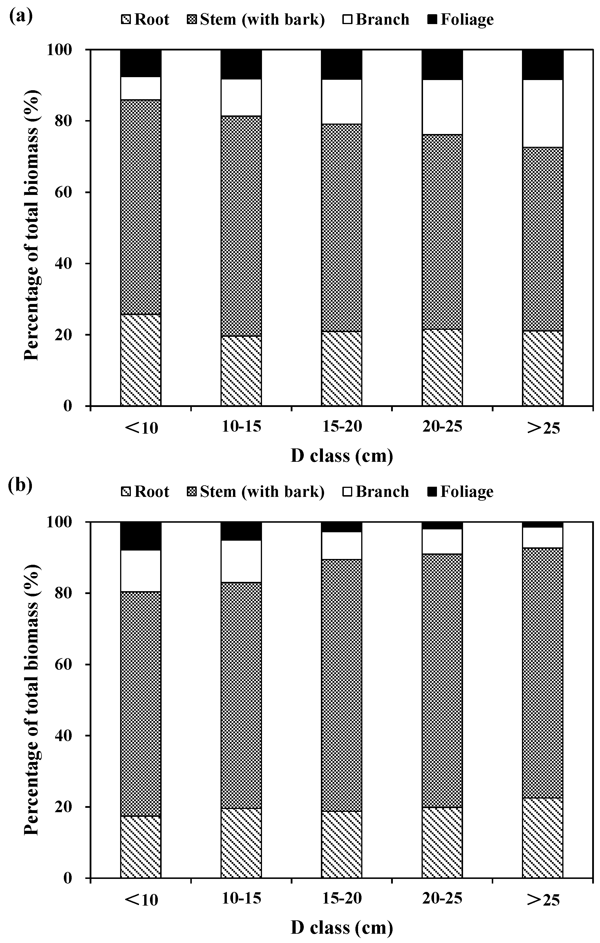
3.1. Biomass Partitioning

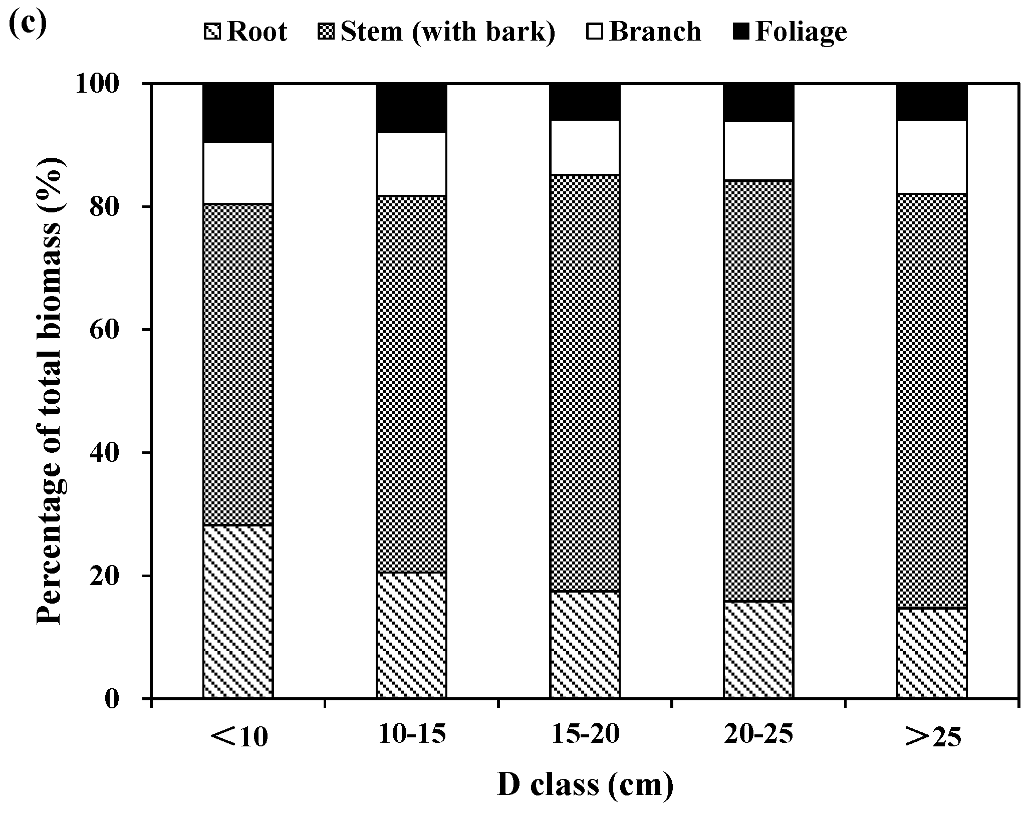
The relative partitioning of tree components to total tree biomass was also computed for the three species across tree diameter classes (Figure 2). For Korean pine, the relative contribution of stem (with bark) biomass to total biomass increased from about 50% for large diameter classes to 60% for small and medium diameter classes. The proportion of root biomass is about 25% for the small diameter class and 20% for the medium and large diameter class. The proportion of branch biomass increased from 7% for the small diameter class and to 19% for the large diameter class. However, the relative contribution of foliage biomass increased marginally with tree diameter classes, because the differences of this relative contribution were not significant among tree diameter classes (Figure 2a). For larch, the proportions of stem and root biomass increased from 63% and 17% for the small diameter class, and to 70% and 21% for medium and large diameter classes, respectively. However, the proportions of branch and foliage biomass decreased from about 12% and 7% for the small diameter class to 6% and 2% for the large diameter class, respectively (Figure 2b). For Mongolian pine, the proportions of root and foliage biomass decreased from 25% and 9% for the small diameter class, and to 15% and 6% for the large diameter class, respectively; however, the proportions of stem biomass increased from 52% for the small diameter class and to 68% for large diameter class. The proportion of branch biomass was greater for the smallest and largest diameter classes, and lesser for the medium diameter class (Figure 2c).

In general, stem biomass had the largest relative contribution to total biomass, while foliage biomass had the smallest relative proportion for the three plantation species. For Korean pine, the proportion was 57% for stem, 22% for root, 13% for branch, and 8% for foliage. For larch, the proportion was 67% for stem, 20% for root, 9% for branch, and 4% for foliage. For Mongolian pine, the proportion was 63% for stem, 20% for root, 10% for branch, and 7% for foliage. On average, the aboveground (i.e., the sum of stems, branches and foliage) biomass was usually above 75% of the total biomass, while the belowground biomass (i.e., roots) was below 25% of the total biomass.

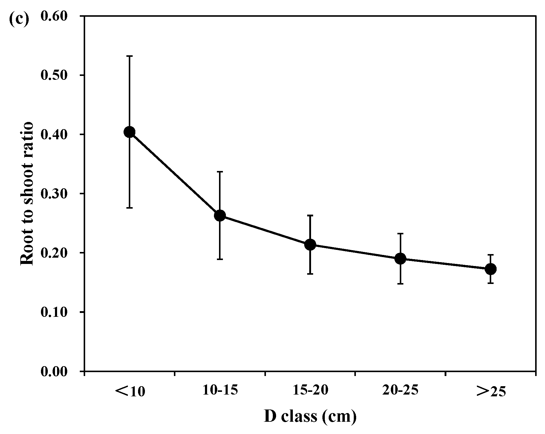
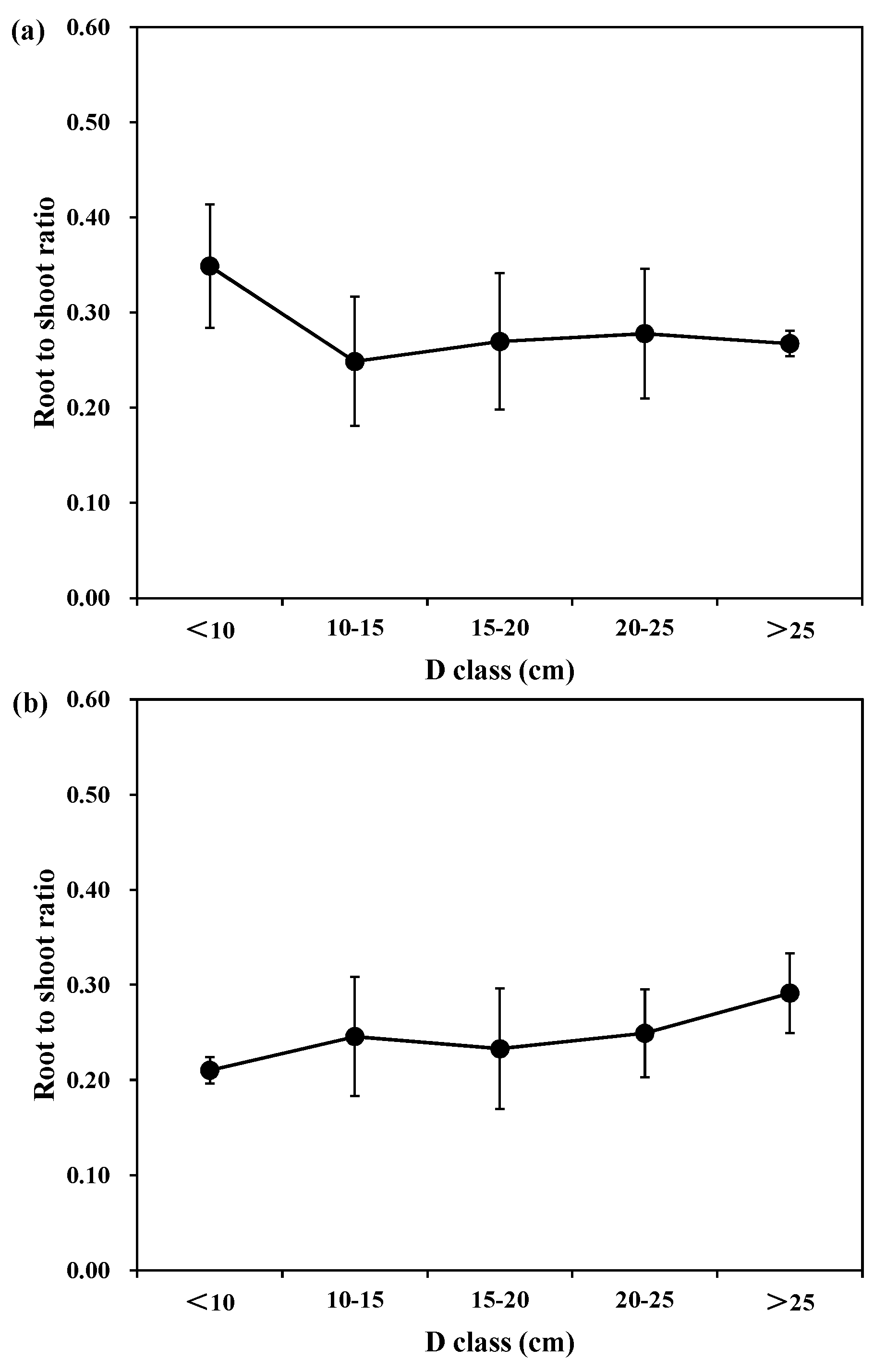
Figure 3 shows the individual root-to -hoot ratio of each tree species in different diameter and age classes. For different diameter classes, the mean root to shoot biomass ratios were 0.35, 0.25, 0.27, 0.28, and 0.27 for Korean pine; 0.21, 0.25, 0.23, 0.25, and 0.29 for larch; and 0.40, 0.26, 0.21, 0.19, and 0.17 for Mongolian pine in D < 10 cm, 10 < D < 15 cm, 15 < D < 20 cm, 20 < D < 25 cm, and D > 25 cm, respectively. Thus, there was a decline in the relative root biomass with the different diameter classes for Korean pine and Mongolian pine, and an increase in the relative root biomass for larch. However, the differences between the medium and large trees were minimal.

3.2. Biomass Additive Systems

With the likelihood analysis, we compared the appropriateness of the two error structures of the two allometric biomass equations (i.e., W = a × D^b and W = a × D^b × H^c) for each of the three species, following the method of Xiao et al. [31]. The information statistics (ΔAICc) of the likelihood analysis are found in Table 3. The results indicated that using the LR was favored over NLR to construct the biomass systems (Table 3). In this study, we developed two additive systems of biomass equations for the three species. The first additive system (i.e., Equation (1), System 1) of biomass equations was fitted in order to estimate individual tree biomass (kg/tree) from tree diameter D only. The second system (i.e., Equation (2), System 2) enabled the estimation of individual tree biomass from both tree diameter (D) and total height (H).

SUR was used to guarantee the additivity property of the tree biomass equations. The independent variable D only or D-H were included in the different biomass component equations (i.e., stems, roots, branches, and foliage), as well as in the total biomass equation. The additivity was guaranteed by setting three constraints to the parameters of the two additive systems of biomass equations in this study.

After applying logarithmic transformation, the coefficient estimates and goodness-of-fit statistics (i.e., R_a² and RMSE) of two additive systems for the three species obtained by SUR are shown in

Table 4. Model coefficient estimates and goodness-of-fit statistics of log-transformed biomass equations with three constraints, using the SUR estimation method.

Tree Species	System Types	Biomass Components	Parameters									Ra2	RMSE
			${\mathit{a}}_{\mathit{i}\mathbf{1}}^{\ast }$			${\mathit{b}}_{\mathit{i}\mathbf{2}}^{\ast }$			${\mathit{c}}_{\mathit{i}\mathbf{3}}^{\ast }$
			Estimate	SE	p Value	Estimate	SE	p Value	Estimate	SE	p Value
Korean pine	System 1	Total	-	-	-	-	-	-	-	-	-	0.972	0.11
		Aboveground	-	-	-	-	-	-	-	-	-	0.971	0.12
		Root	−3.2305	0.1741	<0.0001	2.2295	0.0601	<0.0001	-	-	-	0.865	0.26
		Stem	−2.4644	0.1155	<0.0001	2.2884	0.0392	<0.0001	-	-	-	0.957	0.13
		Branch	−6.6336	0.1800	<0.0001	3.2232	0.0614	<0.0001	-	-	-	0.908	0.29
		Foliage	−5.2441	0.1635	<0.0001	2.5788	0.0554	<0.0001	-	-	-	0.897	0.24
		Crown	-	-	-	-	-	-	-	-	-	0.916	0.25
	System 2	Total	-	-	-	-	-	-	-	-	-	0.975	0.11
		Aboveground	-	-	-	-	-	-	-	-	-	0.974	0.11
		Root	−3.6081	0.2375	<0.0001	2.2338	0.1012	<0.0001	0.1476	0.1571	<0.3497	0.868	0.26
		Stem	−3.0787	0.1431	<0.0001	2.0435	0.0496	<0.0001	0.5406	0.0797	<0.0001	0.970	0.11
		Branch	−6.0711	0.2512	<0.0001	3.4359	0.0836	<0.0001	−0.4892	0.1427	<0.0009	0.913	0.28
		Foliage	−4.9679	0.2389	<0.0001	2.6265	0.0790	<0.0001	−0.1735	0.1338	<0.1974	0.900	0.23
		Crown	-	-	-	-	-	-	-	-	-	0.920	0.24
Larch	System 1	Total	-	-	-	-	-	-	-	-	-	0.966	0.18
		Aboveground	-	-	-	-	-	-	-	-	-	0.958	0.19
		Root	−5.3510	0.1439	<0.0001	2.9914	0.0496	<0.0001	-	-	-	0.964	0.19
		Stem	−3.7797	0.1531	<0.0001	2.8778	0.0515	<0.0001	-	-	-	0.946	0.24
		Branch	−3.7266	0.1401	<0.0001	2.1147	0.0476	<0.0001	-	-	-	0.898	0.23
		Foliage	−2.3186	0.1495	<0.0001	1.2549	0.0509	<0.0001	-	-	-	0.820	0.20
		Crown	-	-	-	-	-	-	-	-	-	0.911	0.19
	System 2	Total	-	-	-	-	-	-	-	-	-	0.989	0.10
		Aboveground	-	-	-	-	-	-	-	-	-	0.989	0.10
		Root	−5.4519	0.1365	<0.0001	2.6643	0.0902	<0.0001	0.3755	0.1004	<0.0003	0.967	0.18
		Stem	−4.5363	0.0959	<0.0001	1.7008	0.0688	<0.0001	1.4804	0.0713	<0.0001	0.987	0.12
		Branch	−3.3632	0.1260	<0.0001	2.6728	0.1041	<0.0001	−0.7052	0.1082	<0.0001	0.919	0.21
		Foliage	−2.2879	0.1505	<0.0001	1.3369	0.1113	<0.0001	−0.0922	0.1205	<0.4466	0.821	0.20
		Crown	-	-	-	-	-	-	-	-	-	0.925	0.18
Mongolian pine	System 1	Total	-	-	-	-	-	-	-	-	-	0.978	0.15
		Aboveground	-	-	-	-	-	-	-	-	-	0.971	0.18
		Root	−2.6309	0.0876	<0.0001	1.9513	0.0310	<0.0001	-	-	-	0.963	0.16
		Stem	−3.5715	0.0310	<0.0001	2.7203	0.0488	<0.0001	-	-	-	0.952	0.24
		Branch	−4.8200	0.1365	<0.0001	2.5112	0.0468	<0.0001	-	-	-	0.956	0.22
		Foliage	−3.9112	0.1496	<0.0001	2.0327	0.0520	<0.0001	-	-	-	0.923	0.25
		Crown	-	-	-	-	-	-	-	-	-	0.961	0.19
	System 2	Total	-	-	-	-	-	-	-	-	-	0.987	0.11
		Aboveground	-	-	-	-	-	-	-	-	-	0.985	0.13
		Root	−2.5406	0.0886	<0.0001	1.9752	0.0886	<0.0001	−0.0606	0.0611	<0.3242	0.962	0.16
		Stem	−3.7044	0.0882	<0.0001	1.9074	0.0599	<0.0001	0.9412	0.0596	<0.0001	0.981	0.15
		Branch	−4.9247	0.1252	<0.0001	2.8783	0.1252	<0.0001	−0.3612	0.0823	<0.0001	0.963	0.21
		Foliage	−3.9908	0.0823	<0.0001	2.5358	0.0878	<0.0001	−0.5262	0.0883	<0.0001	0.940	0.22
		Crown	-	-	-	-	-	-	-	-	-	0.971	0.17

Note: System 1 is Equation (1) and System 2 is Equation (2); $a_{i1}^{\ast }$, $b_{i2}^{\ast }$ and $c_{i3}^{\ast }$ are regression coefficients, i = 1, 2, 3 and 4.

. The results indicated that all equations in System 1 (D only) fitted the biomass data well, with R_a² > 0.80 and RMSE < 0.30. The best model fittings were obtained in total, aboveground and stem biomass equations, while the worse model fittings were for foliage and branch biomass equations with relatively lower model R_a² and larger RMSE (Table 4).

When the tree height was measured, both D and H were used to develop the second additive system of biomass equations (i.e., Equation (2)). In comparison with the model fitting of Equation (1) (D only), the second additive system (D and H) had a relatively greater R_a² and smaller RMSE for total and sub-total component biomass (Table 4), whereas the stem biomass equation of larch had a greater than 4% increase in R² and a greater than 50% decrease in RMSE by including both D and H. The SE and p-values of the parameter estimation indicated that the parameter c for the predictor H was statistically significant (at α = 0.05) in eight of the twelve models (Table 4). Overall, the addition of tree height increased the accuracy for total, aboveground and stem biomass predictions (R_a² and RMSE, Equations (3) and (4)), of which the increased range of R_a² and RMSE is 0.3%–2% and 0.1%–43% for total biomass of the three species; 0.3%–3% and 8%–49% for aboveground biomass of the three species; and 1%–4% and 18%–50% for stem biomass of the three species, respectively. Adding tree height improved the accuracy for most root, branch, foliage, and crown biomass estimations by no more than 1% in R_a² and 10% in RMSE. Among the three species, the additive system with D or D-H for Mongolian pine had slightly better R_a² than those of other tree species (Table 4).

3.3. Model Validation

The model validation statistics (Equations (7)–(10)) based on the jackknifing residuals of the two additive systems of biomass equations are shown in

Table 5. Validation of log-transformed biomass equations by jackknifing technique.

Tree Species	Components	System 1				System 2
		MPE	MPE%	MAB	MAB%	MPE	MPE%	MAB	MAB%
Korean pine	Total	0.01	0.14	0.09	1.99	0.01	0.14	0.09	1.87
	Aboveground	0.01	0.30	0.09	2.18	0.01	0.31	0.09	2.07
	Root	−0.04	−1.33	0.21	7.43	−0.04	−1.35	0.21	7.82
	Stem	0.01	0.31	0.11	2.70	0.01	0.20	0.09	2.24
	Branch	−0.03	−1.03	0.22	8.94	−0.01	−0.23	0.22	9.11
	Foliage	−0.01	−0.25	0.19	10.45	0.01	0.29	0.19	9.75
	Crown	−0.01	−0.45	0.20	6.47	0.00	0.11	0.19	6.75
Larch	Total	0.03	0.62	0.14	3.02	0.01	0.26	0.08	1.66
	Aboveground	0.03	0.66	0.16	3.41	0.01	0.26	0.08	1.80
	Root	0.01	0.40	0.13	4.89	0.00	0.07	0.12	4.59
	Stem	0.03	0.54	0.20	4.58	0.01	0.21	0.09	2.26
	Branch	0.00	−0.08	0.19	9.01	0.01	0.45	0.17	7.96
	Foliage	0.00	0.26	0.17	15.68	0.00	−0.30	0.17	16.32
	Crown	0.00	0.16	0.15	5.89	0.01	0.44	0.14	5.35
Mongolian pine	Total	0.02	0.37	0.12	2.91	0.02	0.34	0.08	1.85
	Aboveground	0.02	0.47	0.15	3.85	0.02	0.37	0.09	2.10
	Root	−0.01	−0.44	0.10	4.02	−0.01	−0.47	0.09	3.88
	Stem	0.01	0.32	0.20	6.02	0.01	0.33	0.10	2.68
	Branch	−0.02	−0.70	0.19	11.88	−0.02	−0.75	0.18	12.24
	Foliage	0.01	0.49	0.21	15.60	0.02	1.29	0.19	13.47
	Crown	0.00	0.06	0.16	6.71	0.01	0.24	0.14	6.23

Note: System 1 is Equation (1) and System 2 is Equation (2).

, in which the MPE and MPE% represent the average prediction error, and the MAB and MAB% represent the magnitude of prediction error. For all biomass equations of the two additive systems for the three species, the average prediction error, i.e., MPE and MPE%, were close to 0. For total, aboveground and stem biomass of the three species, the magnitude of prediction errors of the two additive systems were relatively small (MAB < 0.2 and MAB% < 7%), and System 2 (Equation (2)) seemed preferable to System 1 (Equation (1)). On the other hand, the biomass equations for root, branch, foliage and crown had less accurate prediction, especially branch and foliage, than those for total, aboveground and stem.

In addition, some researchers suggest the prediction across the diameter classes would be a good way of validating the tree biomass models [41,49]. In this study, the MPE, MPE%, MAB and MAB% in tree components of the two additive systems for the three species are listed in

Table A1. Validation in tree components of log-transformed biomass equations by diameter classes.

Tree Species	D Class	System 1				System 2
		MPE	MPE%	MAB	MAB%	MPE	MPE%	MAB	MAB%
Korean pine	Total
	<10	−0.06	−2.41	0.13	5.77	0.02	1.01	0.13	5.23
	10–15	0.01	0.27	0.10	2.59	−0.01	−0.25	0.10	2.53
	15–20	0.03	0.54	0.10	2.14	0.02	0.41	0.09	2.00
	20–25	0.00	−0.09	0.08	1.56	0.00	−0.05	0.08	1.47
	>25	0.00	−0.03	0.05	0.91	0.01	0.22	0.05	0.82
	Aboveground
	<10	−0.07	−3.31	0.13	7.02	0.01	0.32	0.13	6.55
	10–15	0.06	1.49	0.10	2.65	0.03	0.70	0.09	2.51
	15–20	0.04	0.88	0.10	2.13	0.03	0.71	0.09	2.02
	20–25	−0.01	−0.20	0.09	1.89	0.00	−0.09	0.09	1.80
	>25	−0.01	−0.23	0.06	1.07	0.01	0.17	0.05	1.00
	Root
	<10	−0.03	−2.99	0.18	16.58	0.07	6.43	0.25	26.95
	10–15	−0.18	−7.67	0.32	14.74	−0.17	−7.31	0.32	14.75
	15–20	−0.05	−1.73	0.24	7.98	−0.05	−1.73	0.24	8.01
	20–25	−0.01	−0.29	0.19	5.15	−0.02	−0.57	0.19	5.23
	>25	0.04	0.93	0.07	1.59	0.02	0.57	0.05	1.30
	Stem
	<10	−0.09	−4.78	0.16	9.27	0.02	1.20	0.16	8.18
	10–15	0.06	1.72	0.11	3.11	0.01	0.32	0.10	3.04
	15–20	0.05	1.15	0.13	2.99	0.03	0.69	0.10	2.42
	20–25	−0.01	−0.32	0.09	2.00	−0.01	−0.27	0.07	1.51
	>25	−0.03	−0.67	0.06	1.22	0.00	0.10	0.06	1.16
	Branch
	<10	0.03	−11.62	0.06	21.32	−0.08	28.28	0.12	33.31
	10–15	0.00	−0.25	0.14	8.51	0.06	3.24	0.13	7.06
	15–20	−0.04	−1.34	0.22	8.61	0.00	0.04	0.22	8.54
	20–25	−0.05	−1.52	0.28	9.41	−0.03	−0.99	0.28	9.19
	>25	0.05	1.11	0.13	3.24	0.03	0.78	0.15	3.61
	Foliage
	<10	0.00	−1.49	0.21	60.76	−0.07	48.73	0.23	41.52
	10–15	0.06	3.79	0.17	11.12	0.08	5.21	0.18	11.87
	15–20	0.00	0.22	0.20	9.29	0.02	0.93	0.19	9.04
	20–25	−0.03	−1.08	0.21	8.32	−0.01	−0.52	0.21	8.28
	>25	−0.03	−1.05	0.11	3.35	−0.02	−0.77	0.11	3.29
	Crown
	<10	0.01	2.36	0.12	18.26	−0.08	−15.26	0.17	30.08
	10–15	0.03	1.30	0.10	4.31	0.07	3.16	0.12	4.66
	15–20	−0.01	−0.47	0.20	6.41	0.01	0.43	0.19	6.04
	20–25	−0.04	−0.99	0.24	6.90	−0.02	−0.55	0.24	6.74
	>25	0.02	0.47	0.11	2.53	0.01	0.33	0.13	2.81
Larch	Total
	<10	−0.03	−1.10	0.12	4.02	−0.06	−2.06	0.07	2.44
	10–15	−0.02	−0.50	0.17	4.27	0.05	1.18	0.13	3.22
	15–20	0.07	1.54	0.21	4.41	0.02	0.37	0.09	1.84
	20–25	0.08	1.38	0.12	2.14	0.00	−0.06	0.06	1.05
	>25	−0.03	−0.44	0.10	1.60	0.02	0.38	0.05	0.85
	Aboveground
	<10	−0.04	−1.56	0.12	4.37	−0.07	−2.46	0.07	2.59
	10–15	−0.03	−0.91	0.15	4.04	0.05	1.24	0.12	3.31
	15–20	0.09	1.89	0.24	5.22	0.03	0.55	0.09	2.07
	20–25	0.09	1.65	0.14	2.60	0.00	−0.08	0.06	1.19
	>25	−0.04	−0.69	0.12	2.05	0.02	0.32	0.05	0.92
	Root
	<10	0.02	1.63	0.15	12.87	−0.02	−1.96	0.12	9.39
	10–15	0.02	0.84	0.27	12.14	0.03	1.36	0.26	11.40
	15–20	0.00	−0.13	0.14	4.70	−0.03	−0.96	0.14	4.46
	20–25	0.02	0.53	0.08	2.02	−0.01	−0.22	0.08	2.11
	>25	0.01	0.31	0.04	0.93	0.04	0.77	0.06	1.23
	Stem
	<10	−0.02	−0.94	0.16	6.54	−0.05	−2.16	0.07	3.01
	10–15	−0.07	−2.17	0.21	6.28	0.04	1.21	0.15	4.62
	15–20	0.09	2.06	0.29	6.70	0.03	0.63	0.10	2.35
	20–25	0.09	1.65	0.17	3.24	−0.02	−0.38	0.08	1.45
	>25	−0.04	−0.75	0.14	2.48	0.03	0.48	0.07	1.12
	Branch
	<10	−0.12	−16.70	0.12	23.24	−0.11	−14.41	0.16	25.94
	10–15	0.10	5.58	0.22	12.62	0.05	2.76	0.14	8.43
	15–20	−0.08	−3.68	0.20	9.03	−0.05	−2.07	0.14	6.57
	20–25	0.04	1.48	0.20	7.23	0.10	3.46	0.22	7.75
	>25	−0.05	−1.65	0.15	4.67	−0.08	−2.51	0.14	4.34
	Foliage
	<10	−0.08	−24.25	0.08	31.10	−0.08	−25.80	0.08	31.82
	10–15	0.01	1.65	0.18	24.90	0.01	0.63	0.19	26.89
	15–20	−0.04	−2.86	0.19	17.20	−0.04	−3.19	0.20	18.06
	20–25	0.04	2.35	0.20	12.99	0.03	2.10	0.20	12.98
	>25	0.00	−0.12	0.10	5.72	−0.02	−1.05	0.11	5.96
	Crown
	<10	−0.10	−8.34	0.10	9.09	−0.10	−7.85	0.11	9.39
	10–15	0.08	3.79	0.16	7.66	0.04	2.02	0.13	5.99
	15–20	−0.06	−2.49	0.16	6.31	−0.04	−1.50	0.13	5.05
	20–25	0.05	1.55	0.17	5.47	0.09	2.91	0.18	5.61
	>25	−0.04	−1.18	0.12	3.59	−0.07	−1.95	0.12	3.49
Mongolian pine	Total
	<10	0.02	0.96	0.15	6.02	0.03	1.06	0.04	1.55
	10–15	0.00	0.05	0.15	3.76	−0.02	−0.60	0.10	2.71
	15–20	0.09	1.96	0.14	2.89	0.04	0.83	0.09	1.81
	20–25	0.01	0.16	0.11	2.04	0.02	0.37	0.06	1.17
	>25	−0.07	−1.13	0.07	1.21	0.00	0.08	0.06	1.04
	Aboveground
	<10	0.01	0.31	0.21	10.59	0.03	1.17	0.05	2.37
	10–15	0.02	0.55	0.17	4.75	−0.01	−0.21	0.11	3.06
	15–20	0.10	2.25	0.16	3.42	0.04	0.85	0.11	2.41
	20–25	0.01	0.22	0.12	2.35	0.02	0.48	0.06	1.17
	>25	−0.08	−1.38	0.09	1.50	0.00	0.04	0.07	1.17
	Root
	<10	0.05	3.77	0.06	5.00	0.03	1.92	0.04	3.34
	10–15	−0.09	−4.22	0.16	8.36	−0.10	−4.58	0.16	8.20
	15–20	0.03	1.02	0.06	2.07	0.04	1.22	0.07	2.26
	20–25	−0.02	−0.74	0.12	3.63	−0.02	−0.61	0.12	3.73
	>25	0.01	0.17	0.05	1.29	0.01	0.32	0.05	1.23
	Stem
	<10	−0.03	−1.36	0.31	19.87	0.02	1.28	0.05	2.95
	10–15	0.01	0.24	0.24	7.16	−0.03	−0.93	0.14	4.16
	15–20	0.13	2.96	0.21	4.70	0.05	1.08	0.13	3.05
	20–25	0.01	0.28	0.16	3.23	0.04	0.80	0.07	1.52
	>25	−0.13	−2.28	0.13	2.44	−0.01	−0.10	0.07	1.24
	Branch
	<10	0.07	23.61	0.10	36.20	0.08	28.71	0.14	47.77
	10–15	−0.03	−1.84	0.22	14.89	0.01	0.35	0.21	14.14
	15–20	−0.08	−3.36	0.21	9.62	−0.05	−2.04	0.18	8.28
	20–25	−0.08	−2.69	0.19	7.09	−0.10	−3.52	0.20	7.19
	>25	0.10	2.63	0.16	4.16	0.02	0.61	0.12	3.23
	Foliage
	<10	0.02	11.78	0.15	52.96	0.04	21.00	0.15	42.08
	10–15	0.00	−0.21	0.22	17.40	0.05	4.08	0.20	16.09
	15–20	−0.06	−3.19	0.23	12.91	0.00	0.09	0.20	11.10
	20–25	0.03	1.11	0.20	8.23	0.02	0.67	0.18	7.53
	>25	0.10	3.24	0.19	6.08	0.02	0.74	0.16	5.37
	Crown
	<10	0.05	5.36	0.12	16.01	0.07	7.06	0.14	18.08
	10–15	−0.01	−0.46	0.18	8.34	0.03	1.53	0.17	8.10
	15–20	−0.06	−1.97	0.16	5.68	−0.01	−0.47	0.12	4.19
	20–25	−0.03	−0.91	0.16	4.72	−0.05	−1.48	0.16	4.77
	>25	0.10	2.46	0.15	3.53	0.03	0.63	0.11	2.53

Note: System 1 is Equation (1) and System 2 is Equation (2).

. Taking the Korean pine as an example, the results indicated that for total biomass, System 2 reduced the prediction error for most diameter classes, but MPE and MPE% increased slightly in the largest diameter class (D > 25 cm); for aboveground biomass, adding tree height into biomass system reduced the prediction error in all classes; for root biomass, System 2 only reduced the prediction error in D > 25 cm; for stem biomass, in all diameters System 2 reduced the prediction error; for branch, foliage and crown biomass, System 2 reduced the prediction error in all but the smallest diameter class (Table A1). The validation of the other plantation species had similar results.

If a log-transformed biomass model is fitted to biomass data, a correction factor (i.e., CF = exp(σ²/2)) is commonly used to correct for the systematic bias introduced by anti-log transformation. However, Madgwick and Satoo [50] found that anti-log transformation tended to overestimate biomass by applying the correction factor, and suggested that the correction factor might be ignored if the bias was relatively small compared to the overall variation in the estimate of biomass. In this study, the values of the correction factor (i.e., CF = exp(σ²/2)) of all biomass equations were less than 1.04, and the percent biases (see [51], Equation (4)) were relatively small ranging from 0.6% to 4.1% (not shown). Thus, the CF was not applied for the three species in this study.

4. Discussion

We observed a diameter-related pattern in the changes of biomass partitioning among individual aboveground tree components. For larch and Mongolian pine, the results showed that the relative proportion of stem biomass in larger trees was greater across different tree sizes, whereas the crown biomass in larger trees was smaller than those in smaller trees. However, for Korean pine, these findings were not expected and were different from those of other species in general. The main reasons may be (1) the pinecone is an important product of Korean pine. To get more cone production, the older stands of Korean pine need heavier thinning to increase growing space for larger Korean pine trees, which may change the crown profile and the ratio of crown biomass to stems; and (2) the tree climbing and cone taking in the cone collection process may affect tree height growth. Overall, the increase or decrease in the stem, branch, and foliage biomass over different diameter classes found in this study supported the findings of previous studies [17,29,42]. There are obvious differences in partitioning of different biomass components. The belowground biomass (i.e., roots) is a particularly important part of total biomass. The proportion of belowground to total biomass rarely exceeds 30% for most coniferous tree species [29,52]. Our results were consistent with the literature of biomass partitioning. The root to shoot biomass ratios found in our study (0.17–0.40) were similar to the range reported for other coniferous species (0.18–0.35) [29,52,53]. It is crucial to accurately estimate the total biomass, and the root to shoot biomass ratios can be an important predictor for root biomass.

Our likelihood analysis showed that data sets of the total, sub-total and components biomass in trees supported a multiplicative error structure so that linear regression on log-transformed data was more appropriate. Our findings were consistent with previous studies that multiplicative error structure is assumed in biomass allometric equations [4,11,29,51,54]. The likelihood analysis proposed by several authors [31,32] is a good method to verify the error structure of tree biomass data. However, it has not been widely applied in foresty.

Based on the multiplicative error structure of the biomass data, we constructed two additive systems of log-transformed models (Equations (1) and (2)), which were validated using the jackknifing technique. The allometric equation using D as the only predictor is simple in equation form (i.e., Equation (1)), easy to fit to biomass data, requires only basic forest inventory data to apply in practice, and usually provides reasonably accurate predictions for many species and regions [11,14,19,55]. However, adding tree height as an additional predictor into biomass equations can significantly improve the model fitting and performance [21,28]. Our results demonstrated that adding tree height into the additive system marginally improved two-thirds of the biomass equations for the three plantation species, and were consistent with the literature (e.g., [20,26,28]).

The SUR method should be used in model fitting when total biomass is divided into two parts (aboveground and belowground biomass), aboveground is divided into smaller parts (e.g., stem and crown), crown biomass is divided into two parts (branch and foliage), and stem biomass is divided into bark and wood. The advantages of using an additive system by SUR to estimate total, sub-total and components include: (1) prediction for the components’ biomass sum to the prediction for the total or sub-total biomass; (2) the inherent correlation among biomass components measured on the same sample trees is considered; (3) the parameter estimation is more efficient; and (4) no single biomass component is estimated beyond the total or sub-total biomass [10,34,35]. However, the additivity of biomass equations has not always been addressed when predicting tree total and component biomass.

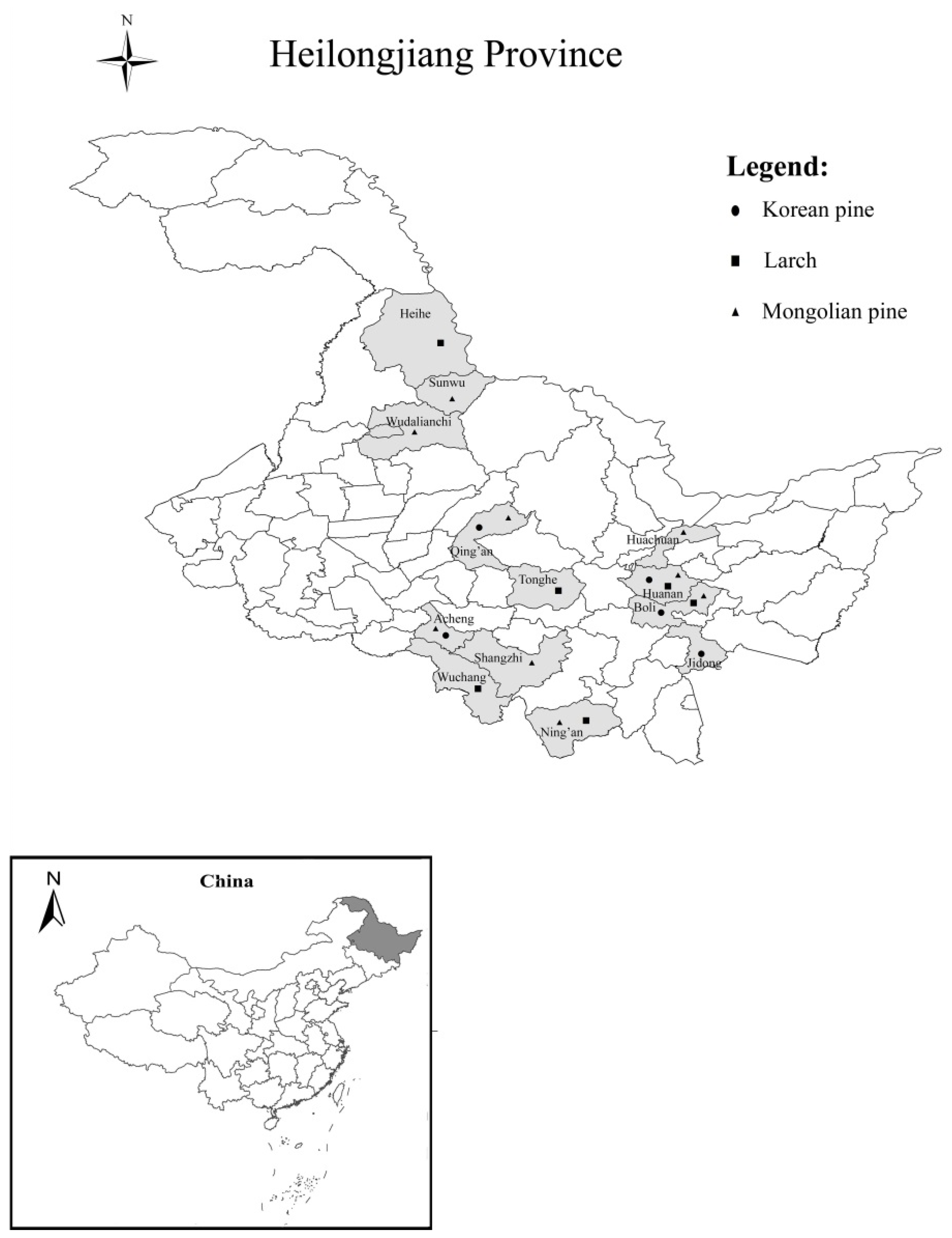
To date, few biomass equations exist for the three coniferous plantation species of northeastern China, especially Mongolian pine. Wang [11] developed biomass equations using D as the only predictor for Korean pine and larch in plantation forest from the Maoershan Ecosystem Research Station of the Northeast Forestry University in Heilongjiang Province, China, which is part of Changbai Mountains. However, his sample size was only ten trees for each species and the biomass equations derived from the sample data were not additive. Our research developed the additive systems of biomass equations for the two species in natural forests in the Xiaoxing’an Mountains, and Changbai Mountains, located in Heilongjiang Province and Jilin Province of China, and the sample sizes in Dong et al. 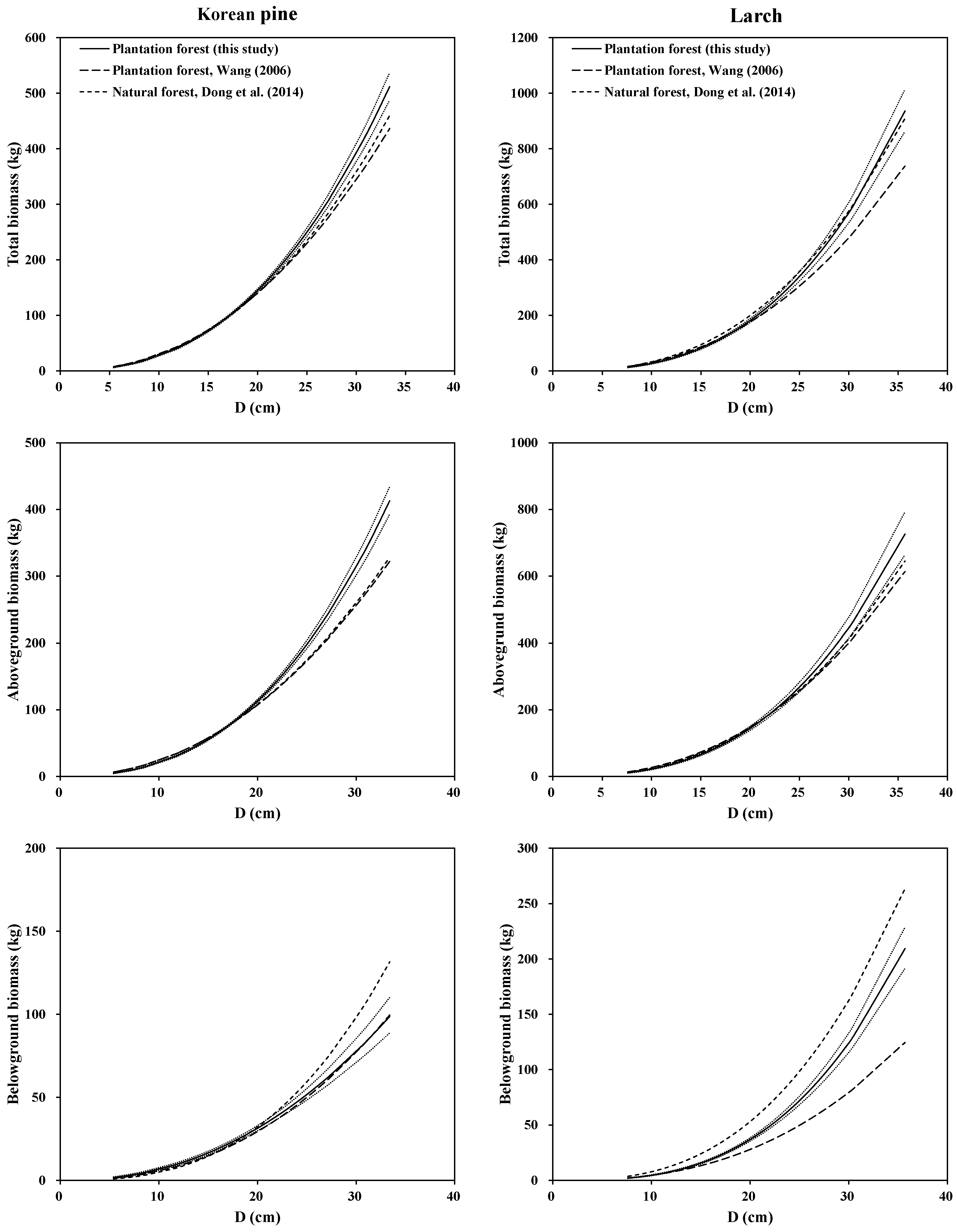[33] was 42 trees for Korean pine and 122 trees for larch in the natural forests, respectively. A graphical analysis of total, aboveground and belowground (root) biomass equations illustrated the differences among our models (System 1) in this study, with Wang [11]’s biomass equations and Dong et al. [33]’s biomass equations for the two species (Figure 4). It is clear that the three models in different forest origins produced different predictions for the root biomass for both species. The models of Korean pine and larch in planted and natural forest produced similar predictions for the aboveground biomass, and most of the mean predicted biomass of Wang’s equations fell into the 95% confidence intervals of mean prediction by our equations. However, our models for the two species in plantations and natural stands yielded higher predictions for the total biomass than Wang’s models for both species, especially for large-sized trees. The possible reasons may be: (1) data of three studies came from different sampling sites; (2) each species of three studies came from different forests; (3) even the two species in plantations were different; and (4) difference in the sample number and sample size range. These may lead to the differences in terms of tree root morphologic features, soil conditions and growth process [10,54,56,57]. Overall, site, stand origin, and stand structural characteristics of the study trees may also play an important role in biomass estimation and partitioning.

5. Conclusions

In this study, we analyzed the biomass partitioning of aboveground and belowground components across diameter classes for the three coniferous species growing in pure plantations in northeastern P.R. China. Our results were consistent with the literature such that (1) partitioning of aboveground and belowground biomass into various tree components changed considerably with tree diameter; (2) stem biomass for the three species accounted for the largest proportion of total biomass. Among them the relative proportion of stem for larch and Mongolian pine increased with tree diameter, and the relative proportion of foliage and branch decreased, while the proportion patterns of stem, branch and foliage biomass were opposite for Korean pine; and (3) the contribution of root biomass to total tree biomass was rather variable, and the root to shoot ranged from 0.17 to 0.40.

The choice between linear regression on log-transformed data (LR) or nonlinear regression on original data (NLR) depends on the model error structure. We used the likelihood analysis outlined by Xiao et al. [31] to assess the model error structure of tree biomass equations. The results indicated that the multiplicative error structure was preferable so that logarithmic transformation was necessary. Then two additive biomass systems were developed for the three species. System 1 used tree diameter D as the only predictor, and System 2 included both tree diameter D and total height H as the predictors. As expected, the accuracy of the biomass component equations differed for the two additive systems across the three species. The mean of all models R_a² was > 0.94 for System 1 (D only) and > 0.95 for System 2 (D and H). The model root mean square error (RMSE) was relatively smaller for total, aboveground and stem biomass equations, but larger for root, branch, foliage, and crown biomass. Overall, adding tree height into the system of biomass equations can marginally improve model fitting and performance, especially for total, aboveground and stem biomass.

References

1. Wang, X.; Fang, J.; Zhu, B. Forest biomass and root-shoot allocation in northeast China. For. Ecol. Manag. 2008, 255, 4007–4020. [Google Scholar] [CrossRef]
2. Schall, P.; Lödige, C.; Beck, M.; Ammer, C. Biomass allocation to roots and shoots is more sensitive to shade and drought in European beech than in Norway spruce seedlings. For. Ecol. Manag. 2012, 266, 246–253. [Google Scholar] [CrossRef]
3. Cai, S.; Kang, X.; Zhang, L. Allometric models for aboveground biomass of ten tree species in northeast China. Ann. For. Res. 2013, 56, 105–122. [Google Scholar]
4. Cienciala, E.; Centeio, A.; Blazek, P.; Gomes Soares, M.D.C.; Russ, R. Estimation of stem and tree level biomass models for Prosopis juliflora/pallida applicable to multi-stemmed tree species. Trees 2013, 27, 1061–1070. [Google Scholar] [CrossRef]
5. Bond-Lamberty, B.; Wang, C.; Gower, S.T. Net primary production and net ecosystem production of a boreal black spruce wildfire chronosequence. Glob. Chang. Biol. 2004, 10, 473–487. [Google Scholar] [CrossRef]
6. Pregitzer, K.S.; Euskirchen, E.S. Carbon cycling and storage in world forests: Biome patterns related to forest age. Glob. Chang. Biol. 2004, 10, 2052–2077. [Google Scholar] [CrossRef]
7. Mu, C.; Lu, H.; Wang, B.; Bao, X.; Cui, W. Short-term effects of harvesting on carbon storage of boreal Larix gmelinii-Carex schmidtii forested wetlands in Daxing’anling, northeast China. For. Ecol. Manag. 2013, 293, 140–148. [Google Scholar] [CrossRef]
8. Konopka, B.; Pajtik, J.; Noguchi, K.; Lukac, M. Replacing Norway spruce with European beech: A comparison of biomass and net primary production patterns in young stands. For. Ecol. Manag. 2013, 302, 185–192. [Google Scholar] [CrossRef]
9. Bond-Lamberty, B.; Wang, C.; Gower, S.T. Aboveground and belowground biomass and sapwood area allometric equations for six boreal tree species of northern Manitoba. Can J. For. Res. 2002, 32, 1441–1450. [Google Scholar] [CrossRef]
10. Bi, H.; Turner, J.; Lambert, M.J. Additive biomass equations for native eucalypt forest trees of temperate Australia. Trees 2004, 18, 467–479. [Google Scholar] [CrossRef]
11. Wang, C. Biomass allometric equations for 10 co-occurring tree species in Chinese temperate forests. For. Ecol. Manag. 2006, 222, 9–16. [Google Scholar] [CrossRef]
12. Alvarez, E.; Duque, A.; Saldarriaga, J.; Cabrera, K.; Salas, G.D.L.; Valle, I.D.; Lema, A.; Moreno, F.; Orrego, S.; Rodríguez, L. Tree above-ground biomass allometries for carbon stocks estimation in the natural forests of Colombia. For. Ecol. Manag. 2012, 267, 297–308. [Google Scholar] [CrossRef]
13. Lambert, M.C.; Ung, C.H.; Raulier, F. Canadian national tree aboveground biomass equations. Can. J. For. Res. 2005, 35, 1996–2018. [Google Scholar] [CrossRef]
14. Jenkins, J.C.; Chojnacky, D.C.; Heath, L.S.; Birdsey, R.A. National-scale biomass estimators for United States tree species. For. Sci. 2003, 49, 12–35. [Google Scholar]
15. Kenzo, T.; Furutani, R.; Hattori, D.; Kendawang, J.J.; Tanaka, S.; Sakurai, K.; Ninomiya, I. Allometric equations for accurate estimation of above-ground biomass in logged-over tropical rainforests in Sarawak, Malaysia. J. For. Res. 2009, 14, 365–372. [Google Scholar] [CrossRef]
16. Fatemi, F.R.; Yanai, R.D.; Hamburg, S.P.; Vadeboncoeur, M.A.; Arthur, M.A.; Briggs, R.D.; Levine, C. Allometric equations for young northern hardwoods: The importance of age-specific equations for estimating aboveground biomass. Can. J. For. Res. 2011, 41, 881–891. [Google Scholar] [CrossRef]
17. Blujdea, V.N.B.; Pilli, R.; Dutca, I.; Ciuvat, L.; Abrudan, I.V. Allometric biomass equations for young broadleaved trees in plantations in Romania. For. Ecol. Manag. 2012, 264, 172–184. [Google Scholar] [CrossRef]
18. Brown, S. Measuring carbon in forests: Current status and future challenges. Environ. Pollut. 2002, 116, 363–372. [Google Scholar] [CrossRef]
19. Ter-Mikaelian, M.T.; Korzukhin, M.D. Biomass equations for sixty-five North American tree species. For. Ecol. Manag. 1997, 97, 1–24. [Google Scholar] [CrossRef]
20. Cole, T.G.; Ewel, J.J. Allometric equations for four valuable tropical tree species. For. Ecol. Manag. 2006, 229, 351–360. [Google Scholar] [CrossRef]
21. Wang, X.; Fang, J.; Tang, Z.; Zhu, B. Climatic control of primary forest structure and D-height allometry in Northeast China. For. Ecol. Manag. 2006, 234, 264–274. [Google Scholar] [CrossRef]
22. Zhou, X.; Brandle, J.R.; Schoeneberger, M.M.; Awada, T. Developing above-ground woody biomass equations for open-grown, multiple-stemmed tree species: Shelterbelt-grown Russian-olive. Ecol. Model. 2007, 202, 311–323. [Google Scholar] [CrossRef]
23. Zhang, C.; Peng, D.L.; Huang, G.S.; Zeng, W.S. Developing aboveground biomass equations both compatible with tree volume equations and additive systems for single-trees in poplar plantations in Jiangsu province, China. Forests 2016, 7, 32. [Google Scholar] [CrossRef]
24. Peria, P.L.; Verónica, G.; Pastur, G.M.; Lencinas, M.V. Carbon accumulation along a stand development sequence of Nothofagus antarctica forests across a gradient in site quality in Southern Patagonia. For. Ecol. Manag. 2010, 260, 229–237. [Google Scholar] [CrossRef]
25. Verónica, G.; Louis, P.P.; Gerardo, R. Allometric relations for biomass partitioning of Nothofagus antarctica trees of different crown classes over a site quality gradient. For. Ecol. Manag. 2010, 259, 1118–1126. [Google Scholar]
26. Battulga, P.; Tsogtbaatar, J.; Dulamsuren, C.; Hauck, M. Equations for estimating the above-ground biomass of Larix sibirica in the forest-steppe of Mongolia. J. For. Res. 2013, 24, 431–437. [Google Scholar] [CrossRef]
27. Menendez-Miguelez, M.; Canga, E.; Barrio-Anta, M.; Majada, J.; Alvarez-Alvarez, P. A three level system for estimating the biomass of Castanea sativa Mill. coppice stands in north-west Spain. For. Ecol. Manag. 2013, 291, 417–426. [Google Scholar] [CrossRef]
28. Bi, H.; Murphy, S.; Volkova, L.; Weston, C.; Fairman, T.; Li, Y.; Law, R.; Norris, J.; Lei, X.; Caccamo, G. Additive biomass equations based on complete weighing of sample trees for open eucalypt forest species in south-eastern Australia. For. Ecol. Manag. 2015, 349, 106–121. [Google Scholar] [CrossRef]
29. Wang, J.; Zhang, C.; Xia, F.; Zhao, X.; Wu, L.; Gadow, K.V. Biomass structure and allometry of Abies nephrolepis (Maxim) in Northeast China. Silva Fenn. 2011, 45, 211–226. [Google Scholar] [CrossRef]
30. Lai, J.; Yang, B.; Lin, D.; Kerkhoff, A.J.; Ma, K. The allometry of coarse root biomass: Log-transformed linear regression or nonlinear regression? PLoS ONE 2013, 8, e77007. [Google Scholar] [CrossRef] [PubMed]
31. Xiao, X.; White, E.P.; Hooten, M.B.; Durham, S.L. On the use of log-transformation vs. nonlinear regression for analyzing biological power laws. Ecology 2011, 92, 1887–1894. [Google Scholar] [CrossRef] [PubMed]
32. Ballantyne, F.T. Evaluating model fit to determine if logarithmic transformations are necessary in allometry: A comment on the exchange between Packard (2009) and Kerkhoff and Enquist (2009). J. Theor. Biol. 2013, 317, 418–421. [Google Scholar] [CrossRef] [PubMed]
33. Dong, L.; Zhang, L.; Li, F. A compatible system of biomass equations for three conifer species in Northeast, China. For. Ecol. Manag. 2014, 329, 306–317. [Google Scholar] [CrossRef]
34. Parresol, B.R. Assessing tree and stand biomass: A review with examples and critical comparisons. For. Sci. 1999, 45, 573–593. [Google Scholar]
35. Parresol, B.R. Additivity of nonlinear biomass equations. Can. J. For. Res. 2001, 31, 865–878. [Google Scholar] [CrossRef]
36. Tang, S.; Li, Y.; Wang, Y. Simultaneous equations, error-in-variable models, and model integration in systems ecology. Ecol. Mod. 2001, 142, 285–294. [Google Scholar] [CrossRef]
37. Carvalho, J.P.; Parresol, B.R. Additivity in tree biomass components of Pyrenean oak (Quercus pyrenaica Willd.). For. Ecol. Manag. 2003, 179, 269–276. [Google Scholar] [CrossRef]
38. Návar, J. Biomass component equations for Latin American species and groups of species. Ann. For. Sci. 2009, 66, 208–216. [Google Scholar] [CrossRef]
39. Russell, M.B.; Burkhart, H.E.; Amateis, R.L. Biomass partitioning in a miniature-scale loblolly pine spacing trial. Can. J. For. Res. 2009, 39, 320–329. [Google Scholar] [CrossRef]
40. Castedo-Dorado, F.; Gomez-Garcia, E.; Dieguez-Aranda, U.; Barrio-Anta, M.; Crecente-Campo, F. Aboveground stand-level biomass estimation: A comparison of two methods for major forest species in northwest Spain. Ann. For. Sci. 2012, 69, 735–746. [Google Scholar] [CrossRef]
41. Li, H.; Zhao, P. Improving the accuracy of tree-level aboveground biomass equations with height classification at a large regional scale. For. Ecol. Manag. 2013, 289, 153–163. [Google Scholar] [CrossRef]
42. Son, Y.; Hwang, J.W.; Kim, Z.S.; Lee, W.K.; Kim, J.S. Allometry and biomass of Korean pine (Pinus koraiensis) in central Korea. Bioresour. Technol. 2001, 78, 251–255. [Google Scholar] [CrossRef]
43. Fu, L.; Zeng, W.; Zhang, H.; Wang, G.; Lei, Y.; Tang, S. Generic linear mixed-effects individual-tree biomass models for Pinus massoniana in southern China. South For. 2014, 76, 47–56. [Google Scholar]
44. Zeng, W.S. Using nonlinear mixed model and dummy variable model approaches to construct origin-based single tree biomass equations. Trees 2014, 29, 275–283. [Google Scholar] [CrossRef]
45. SAS Institute Inc. SAS/ETS® 9.3. User’s Guide; SAS Institute Inc.: Cary, NC, USA, 2011. [Google Scholar]
46. Balboa-Murias, M.Á.; Rodríguez-Soalleiro, R.; Merino, A.; Álvarez-González, J.G. Temporal variations and distribution of carbon stocks in aboveground biomass of radiata pine and maritime pine pure stands under different silvicultural alternatives. For. Ecol. Manag. 2006, 237, 29–38. [Google Scholar] [CrossRef]
47. Dong, L.; Zhang, L.; Li, F. A Three-step proportional weighting system of nonlinear biomass equations. For. Sci. 2015, 61, 35–45. [Google Scholar]
48. Quint, T.C.; Dech, J.P. Allometric models for predicting the aboveground biomass of Canada yew (Taxus canadensis Marsh.) from visual and digital cover estimates. Can. J. For. Res. 2010, 40, 2003–2014. [Google Scholar] [CrossRef]
49. Kozak, A.; Kozak, R. Does cross validation provide additional information in the evaluation of regression models? Can. J. For. Res. 2003, 33, 976–987. [Google Scholar] [CrossRef]
50. Madgwick, H.; Satoo, T. On estimating the aboveground weights of tree stands. Ecology 1975, 56, 1446–1450. [Google Scholar] [CrossRef]
51. Zianis, D.; Xanthopoulos, G.; Kalabokidis, K.; Kazakis, G.; Ghosn, D.; Roussou, O. Allometric equations for aboveground biomass estimation by size class for Pinus brutia Ten. trees growing in North and South Aegean Islands, Greece. Eur. J. For. Res. 2011, 130, 145–160. [Google Scholar] [CrossRef]
52. Cairns, M.A.; Brown, S.; Helmer, E.H.; Baumgardner, G.A. Root biomass allocation in the world’s upland forests. Oecologia 1997, 111, 1–11. [Google Scholar] [CrossRef]
53. Vega-Nieva, D.J.; Valero, E.; Picos, J.; Jiménez, E. Modeling the above and belowground biomass of planted and coppiced Eucalytpus globulus, stands in NW Spain. Ann. For. Sci. 2015, 72, 967–980. [Google Scholar] [CrossRef]
54. Zianis, D.; Mencuccini, M. Aboveground biomass relationships for beech (Fagus moesiaca Cz.) trees in Vermio Mountain, Northern Greece, and generalised equations for Fagus sp. Ann. For. Sci. 2003, 60, 439–448. [Google Scholar] [CrossRef]
55. Basuki, T.M.; Laake, P.E.V.; Skidmore, A.K.; Hussin, Y.A. Allometric equations for estimating the above-ground biomass in tropical lowland Dipterocarp forests. For. Ecol. Manag. 2009, 257, 1684–1694. [Google Scholar] [CrossRef]
56. Strong, W.; Roi, G.L. Root-system morphology of common boreal forest trees in Alberta, Canada. Can. J. For. Res. 1983, 13, 1164–1173. [Google Scholar] [CrossRef]
57. Nicoll, B.C.; Ray, D. Adaptive growth of tree root systems in response to wind action and site conditions. Tree Physiol. 1996, 16, 891–898. [Google Scholar] [CrossRef] [PubMed]
Figure 1. Geographical location of study area and plot distribution in Heilongjiang province of China.
Forests 07 00136 g001
Figure 2. Biomass partitioning of aboveground and belowground components across a range of diameter classes (the first column; <10 cm, 10–15 cm, 15–20 cm, 20–25 cm and >25 cm): (a) Korean pine; (b) Larch; and (c) Mongolian pine.
Forests 07 00136 g002aForests 07 00136 g002b
Figure 3. Root to shoot biomass ratios for Korean pine, larch and Mongolian pine across a range of diameter classes (the first column; <10 cm, 10–15 cm, 15–20 cm, 20–25 cm and >25 cm): (a) Korean pine; (b) Larch; and (c) Mongolian pine.
Forests 07 00136 g003aForests 07 00136 g003b
Figure 4. The comparison of model predictions from System 1 in this study, with Wang [11]’s and Dong et al. [33]’s biomass equations for total, aboveground, and root biomass for Korean pine and larch.
Forests 07 00136 g004