Article

Impacts of Forest to Urban Land Conversion and ENSO Phase on Water Quality of a Public Water Supply Reservoir

1
U.S. Department of Agriculture—Agricultural Research Service, Wooton Hall, New Mexico State University, Las Cruces, NM, 88003, USA
2
TetraTech, Inc., 2110 Powers Ferry Rd., Atlanta, GA 30326, USA
3
Auburn University, 206 Tom Corley Bldg., Auburn, AL 36832, USA
4
New Mexico State University, Las Cruces, NM, 88003 USA
*
Author to whom correspondence should be addressed.
These authors contributed equally to this work.
Forests 2016, 7(2), 29; https://doi.org/10.3390/f7020029
Submission received: 15 November 2015 / Revised: 15 January 2016 / Accepted: 18 January 2016 / Published: 27 January 2016
(This article belongs to the Special Issue Forest Management and Water Resources in the Anthropocene)

Abstract

:
We used coupled watershed and reservoir models to evaluate the impacts of deforestation and l Niño Southern Oscillation (ENSO) phase on drinking water quality. Source water total organic carbon (TOC) is especially important due to the potential for production of carcinogenic disinfection byproducts (DBPs). The Environmental Fluid Dynamics Code (EFDC) reservoir model is used to evaluate the difference between daily pre- and post- urbanization nutrients and TOC concentration. Post-disturbance (future) reservoir total nitrogen (TN), total phosphorus (TP), TOC and chlorophyll-a concentrations were found to be higher than pre-urbanization (base) concentrations (p < 0.05). Predicted future median TOC concentration was 1.1 mg·L−1 (41% higher than base TOC concentration) at the source water intake. Simulations show that prior to urbanization, additional water treatment was necessary on 47% of the days between May and October. However, following simulated urbanization, additional drinking water treatment might be continuously necessary between May and October. One of six ENSO indices is weakly negatively correlated with the measured reservoir TOC indicating there may be higher TOC concentrations in times of lower streamflow (La Niña). There is a positive significant correlation between simulated TN and TP concentrations with ENSO suggesting higher concentrations during El Niño.

1. Introduction

Forested watersheds provide essential ecosystem services such as the provision of high quality water. As watershed land becomes increasingly urbanized, valuable filtration services once provided by the forested catchments are lost. Drinking water treatment authorities in locations such as Boston, MA, Portland, OR, and New York, NY recognize the water quality benefits from forested catchments and actively purchase natural land in supplying watersheds. For example, an improvement in turbidity of 30% saved $90,000 to $553,000 per year for drinking water treatment in the Neuse Basin of North Carolina [1]. An analysis of 27 US water suppliers concluded that a reduction from 60% to 10% forest land increased drinking water treatment costs by 211% [2]. The progressive loss of forest ecosystem services risks harm to human health through lowered drinking water quality, as well as increased drinking water treatment cost [2].
One water quality variable of particular interest to water providers is total organic carbon (TOC) because of disinfection byproduct (DBP) formation. Source water TOC is a good indicator of the amount of DBP that may form as a result of chemical disinfection [3]. TOC reacts with chlorine during the disinfection phase of water treatment to form DBPs. Several DBPs have been identified by the US Environmental Protection Agency (US EPA) as probable human carcinogens. Evidence is insufficient to support a causal relationship between chlorinated drinking water and cancer. However, the US EPA concluded that epidemiology studies support a potential association between exposure to chlorinated drinking water and bladder cancer leading to the introduction of the Stage 2 DBP rule. The American Cancer Society (ACS) estimates that there will be about 74,000 new cases of bladder cancer diagnosed in the United States each year [4]. Approximately 2260 drinking water treatment plants nationwide are estimated to make treatment technology changes to comply with the Stage 2 DBP rule [5]. An alternate method to mitigate DBP formation is the management of watershed land to reduce source water TOC [6,7].
While water providers are struggling to maintain low source water TOC concentrations and minimize DBP formation potential, many source water catchments are undergoing rapid forest to urban land use change [8]. The impact of forest to urban land conversion on lotic TOC concentrations varies, however literature reports elevated TN and TP concentrations in urban streams [9]. Elevated nutrient concentrations can support increased algae growth thereby increasing overall TOC in reservoirs regardless of the allochthonous contribution.
Here we assess the impact of forest to urban land conversion on reservoir TOC concentrations at Converse Reservoir, which supplies the drinking water for the City of Mobile, Alabama through the Mobile Area Water and Sewer Systems (MAWSS). MAWSS is one of the >2000 water treatment facilities nationally making changes to comply with the Stage 2 DBP rule because of existing elevated TOC concentrations. Rapid urbanization is occurring in the contributing watershed and urbanization projections concur that the watershed will undergo significant urbanization in the coming decades [8,10,11]. Like other urbanizing watersheds, the concern is that Mobile source water TOC concentrations may increase as watershed urbanization continues.
Along with watershed forest to urban land conversion, changes in reservoir concentrations may be related to variations in ocean-atmosphere oscillation, known as El Niño Southern Oscillation (ENSO). In southern Alabama, interannual variations in precipitation and streamflow are related to ENSO. El Niño events, which occur every 2 to 10 years, are caused by positive sea surface temperature anomalies. Conversely, La Niña events are caused by negative sea surface temperature anomalies (SST). Strong relationships have been established between ENSO and precipitation in certain regions including southern Alabama, ENSO and water temperature and ENSO and streamflow in the Converse watershed [12]. El Niño seasonal precipitation has been shown to be higher than normal and La Niña precipitation in the three southern climate divisions in Alabama [13]. Precipitation during JFM in the La Niña phase is lower than normal for the southern climate divisions [14]. TOC loads from watershed sources have also been linked with ENSO phase and reflect a seasonal component wherein El Niño TOC loads are higher than neutral or La Niña phase loads during Jan-Mar, but lower than La Niña during Aug-Oct [15]. During El Niño events in January to March, the higher precipitation and streamflow could lead to higher nutrient loads delivered to Converse or similar reservoirs.
Changes in precipitation and temperature can have a significant effect on surface water quality [16]. There is a relationship between ENSO phase, precipitation and streamflow in Alabama [13]. Seasonal streamflow is related to both ENSO phase and surface water nutrient loadings [17]. ENSO phase has been found to have strong nitrate concentration, streamflow and precipitation predictive effects in a southeastern U.S. watershed [18]. ENSO phase has been linked to flow, stream temperature, dissolved oxygen and water quality parameters in southeast Alabama and related to ENSO phase for predicting periods restrictive to point-source discharge to limit water quality impairment [19].
Changes in land use can significantly alter the quality of adjacent surface waters [16]. Increased nutrient concentrations are associated with urban streams [9]. However, the relationship between land use and water quality can vary regionally and even on a stream-by-stream basis due to many factors including land use intensity, geology, precipitation patterns. In the greater Converse Watershed urban subwatersheds had higher TP and TN loads and concentrations than undisturbed forested watershed [20,21]. Watershed simulations also support elevated post-urbanization nutrient concentrations [22]. Converse Reservoir response to changing land use was evaluated previously using a BATHTUB reservoir model [23]. Modelers found increased TP and TN loads, changes in trophic state and increased algal blooms.
This study improves upon previous research by evaluating the impacts of two major stressors to water resources of Converse Reservoir simultaneously. Here we concurrently evaluate the impacts of watershed urbanization and ENSO phase on reservoir water quality. The modeling utilized in this study expands previous efforts by utilizing coupled watershed and reservoir models rather than the BATHTUB model [23], simulating the entire year, rather than April to September only, and using a realistic estimate of watershed urbanization, rather than the expectation of 100% land development. This study builds upon previous efforts [15,19] by relating ENSO phase to reservoir, rather than stream, water quality. Reservoir modeling studies most often evaluate nitrogen and phosphorous fractions, but here we simulate TOC, the variable of most interest to drinking water managers. The rigor of modeling efforts used here, the relation to multiple watershed stressors and the incorporation of reservoir water quality serve to enhance our understanding of the relationship between urbanization, ENSO phase and water quality. To evaluate the impact of forest to urban land conversion and ENSO phase on reservoir water quality, linked watershed [24] and reservoir [25] models were used. Daily nutrient concentrations and streamflow from watershed simulations provide input data to estimate the effects on nutrient and TOC concentrations within the reservoir under base and future land use conditions. Total (1992 to 2005) and monthly median TOC concentrations at a source water intake from base and future scenarios were compared. Additionally, six ENSO indices were correlated with (1) measured TOC; (2) simulated pre-urbanization monthly nutrient and reservoir TOC concentrations; and (3) simulated post- urbanization monthly nutrient and TOC concentrations.
The objectives of this study were to (1) utilize linked watershed and reservoir models to test the hypothesis that watershed nutrient loads during future scenarios will lead to increased TOC concentrations and algae growth at the source water intake when compared with base scenarios; (2) evaluate the influence of anticipated forest to urban land use change in terms of the daily and monthly changes in source water nutrient and TOC concentrations; and (3) evaluate the influence of ENSO phase on measured TOC and simulated pre- and post- urbanization TN, TP, chlorophyll-a and TOC concentrations.

Study Area

Converse Reservoir supplies the majority of drinking water for the City of Mobile, Alabama through the Mobile Area Water and Sewer Service (MAWSS). Past concerns about the quality of Converse Reservoir as a supply source for drinking water prompted various scientific investigations [20,21,23,26,27,28]. Tributary and reservoir water quality data were collected by the United States Geological Survey (USGS), Auburn University (AU) and MAWSS under various sampling programs beginning in 1990.
Converse Reservoir was formed in 1952 by impoundment of Big Creek in Mobile County, Alabama with a 37 m high earthen dam. The physical characteristics of the reservoir include: volume 64,100,000 m3, surface area 14.6 km2, mean depth 4.4 m, and maximum depth 15.2 m. Converse Reservoir has two main branches, Big Creek, which is the reservoir mainstem, and Hamilton Creek, which contains the drinking water intake 4.8 km from the reservoir mainstem (
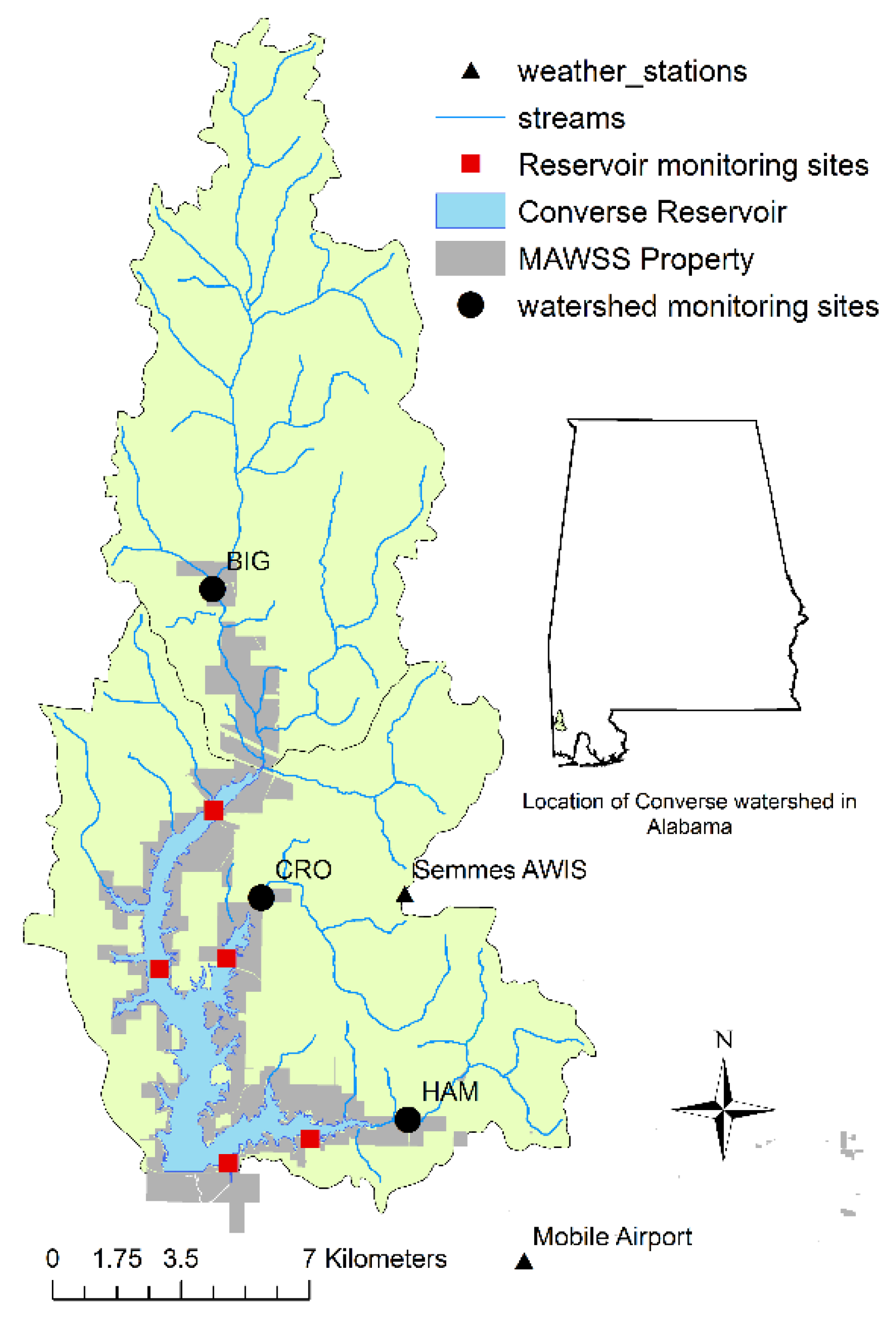
Figure 1).
Figure 1. Monitoring locations, weather stations, and Mobile Area Water and Sewer System (MAWSS) property in the Converse watershed and reservoir located in southwestern Alabama.
Forests 07 00029 g001
Precipitation near the study area is some of the highest in the US, with a 48-year (1957–2005) median monthly precipitation of 12.40 cm (1953–2005). A firm-yield analysis of Converse Reservoir estimated ~5% of the total reservoir volume is from groundwater [29]. Streamflow from the 3 major tributaries has been monitored by USGS gauging stations since 1990.
A 267 km2 watershed drains to the reservoir. Within the watershed there are wetlands, forests, dairy farms, plant nurseries, pecan groves and residential areas using septic tanks for sewage disposal. Watershed soils are generally acidic, low in organic matter content and composed of fine sand or loamy find sand [30]. The eastern watershed boundary extends to within 500 m of Mobile, Alabama city limits. Local, regional and national urbanization studies concur that the study area will likely experience significant urbanization in the coming decades [8,10,11,31].

2. Methods

Long-term simulations using measured hydrologic data were conducted for 1991 to 2005. Environmental Fluid Dynamics Code (EFDC) model simulations were first conducted using uncorrected inflows from the Loading Simulation Program C++ (LSPC) watershed model and water surface elevation. Next, 4 s time-step simulations were conducted using constant outflows. Corrected water surface elevation is recorded daily. After hydrodynamic routines were executed water quality simulations were conducted.

2.1. Software: EFDC Hydrodynamic Model

The EFDC hydrodynamic model was developed at the Virginia Institute of Marine Science beginning in 1988 [25]. EFDC has been applied in various locations, including Chesapeake Bay estuarine system [32], the Neuse Estuary in North Carolina [33] and the Florida Everglades [34]. It has been used in a wide range of environmental studies including simulations of pollutant and pathogenic organism transport, simulation of power plant cooling water discharges, simulation of oyster and crab larvae transport, and evaluation of dredging and dredge spoil disposal alternatives [35]. EFDC has evolved over the past several decades to become one of the most technically defensible and widely used reservoir models available [24]. The EFDC hydrodynamic model provides the hydrologic basis for a number of other water quality models such as Water Quality Analysis Simulation program (WASP5) [36] and the multi-dimensional surface water model (CE-QUAL-ICM) [37]. Details regarding model set-up and theoretical basis are provided in the EFDC User’s Manual [35] and the EFDC Theory and Computation Manual [38].
EFDC is an open-access FORTRAN 77 based hydrodynamic model particularly adept at simulating estuarine and reservoir systems. EFDC is an orthogonal, grid-based model, so model execution requires computation of an orthogonal grid with specified number of vertical layers, which is easiest to create using a specialized program (visual orthogonal grid generator). The model solves three-dimensional, vertically hydrostatic equations of motion with many aspects computationally equivalent to the Blumberg-Mellor model [39]. Multiple text files supply various functions in model computation including control files (efdc.inp, show.inp), grid specification files (cell.inp, depth.inp, gcellmap.inp, dxdy.inp, lxly.inp), and time series files (aser.inp (atmospheric information), pser.inp (surface water elevation), qser.inp (volumetric source-sink). EFDC produces various output file classes, all controlled by the master input file (efdc.inp). Modelers can specify diagnostic output files, restart files, two-dimensional graphic and visualization files and three-dimensional graphic and visualization files.

2.2. Scenarios

The 1992 multi-resolution land cover (MRLC) land cover served as the base (pre-urbanization) scenario for comparison with the future (2020; post-urbanization) scenario (Table 1). The 2020 scenario is based on the population-based housing density forecasts of the Forests On The Edge Project [40]. During base and future simulations only daily LSPC-derived streamflow and TN, TP and TOC loads to Converse Reservoir change [22,41].
Table 1. Comparison of 1992 multi-resolution land cover percentages within the Converse Watershed, AL.
Land Use1992Post-Urbanization
Watershed Area (km2)Watershed (%)Watershed Area (km2)
Urban7.72.9%59.7
Barren0.00.0%0.0
Forest165.661.6%113.6
Pasture45.316.9%45.3
Cropland32.812.2%32.8
wetlands4.81.8%4.8
Water12.54.6%12.5
Total268.7100%268.7

2.3. Model Configuration

2.3.1. Orthogonal Reservoir Model Grid Generation

Reservoir bathymetry data were unavailable so topographic maps, which reflect the watershed prior to reservoir impoundment in 1952, were used to delineate reservoir bathymetry. We imported photographs of the maps into ArcMap Version 9.1 and georeferenced them to 7.5-min topographic maps. VOGG: A Visual Orthogonal Grid Generation Tool for Hydrodynamic and Water Quality Modeling generates the grid required for reservoir modeling [42]. The grid serves as the reference system for EFDC modeling. A total of 575 grid cells in a curvilinear grid array represented the Converse Reservoir (Figure 2). The mean cell width is 178 m (range: 139–208 m) and mean cell height is 186 m (range: 97–390 m).
Figure 2. Grid showing the Converse Reservoir with eight control points and 575 cells used in Environmental Fluid Dynamics Code (EFDC) modeling. Cell colors correspond with bottom elevation in meters above mean sea level. Numbers represent the horizon.
Forests 07 00029 g002

2.3.2. Atmospheric Data

We used hourly local climatological data from the National Climatic Data Center (NCDC) for the Mobile Regional Airport weather station for the monitoring period. Atmospheric input files include hourly barometric pressure, air temperature, dewpoint temperature, rainfall, solar radiation, and cloud cover, wind speed and wind direction.

2.3.3. Reservoir Inflows and Outflows

The input file of streamflow and outflow data (qser.inp) was created using modeled LSPC streamflow. Simulated inflows from all subwatersheds draining to Converse Reservoir were apportioned to one of five inflows (Hamilton Creek, Crooked Creek, Big Creek, Long Branch, and Boggy Branch). The two simulated outflows are dam spillage and pumpage for drinking water treatment, taken from MAWSS records. Water level was the measured water surface elevation during the first day of simulation and fluctuated with each time step during the simulation. Dam and lake seepage and groundwater interaction are not simulated by EFDC and estimated to be negligible. Losses to lake evaporation are approximately equal to precipitation in this humid, subtropical region.

2.3.4. Tributary Water Quality Inputs

Daily TN, TP and TOC concentrations from the watershed model [22] were partitioned into nutrient fractions for the EFDC model based upon measured data for each stream (Table 2).
Table 2. Environmental Fluid Dynamics Code (EFDC) water quality simulation variables and measured data used to partition simulated total nitrogen (TN), total phosphorus (TP) and total organic carbon (TOC) into nutrient fractions.
EFDC Simulation VariableMeasured Data Used to Partition Simulated TN, TP and TOC into Fractions
Green Algae= Daily inflow × 0.002 mg·L−1 × 2.447 = kg·d−1
Refractory Particulate Organic C= TOC (680 ) − DOC (681 ).
Dissolved Organic C= 681
Refractory Particulate Organic P= TP (665 ) − dissolved orthophosphate (671 ) and dissolved organic P (below).
Dissolved Organic P= [dissolved P (666 ) − dissolved orthophosphorus (671 )].
Total Phosphate= TP (665) – organic P (above)
Refractory Particulate Organic N= 20% of the total organic N. TON = ammonium (625 ) − organic N (610 ).
Dissolved Organic N= 80% of the total organic N.
Ammonium N= 610
Nitrate N= 630
Dissolved O2Mean monthly measured dissolved O2 concentrations are used to estimate daily tributary dissolved O2.
indicates USGS parameter code.
Measured data provided the basis for partitioning watershed model TN concentrations into TON, nitrate and ammonium values based upon the following relationship; TN is the sum of inorganic N [nitrate and ammonium] and organic N. Organic N was simulated in either the dissolved or particulate form. TON was assumed to be ~20% particulate and 80% dissolved based upon the measured proportions in samples at Big, Crooked and Hamilton creeks (TON n = 61; DON n = 52). Dissolved and particulate organic P are partitioned based upon the following relationship; TP = particulate organic P + dissolved organic P + orthophosphate. Measured TP, dissolved P and orthophosphorus were used to calculate the percentage of incoming simulated TP as dissolved organic, particulate organic and inorganic (orthophosphate) at all 5 tributaries flowing into Converse Reservoir. Organic C was simulated in particulate and dissolved forms. Measured TOC and DOC data are used to partition the simulated TOC from the watershed model into dissolved and particulate fractions. Daily values of 2 µg·L−1 for green algae chlorophyll-a were input. Measured data provided an estimate of mean monthly dissolved oxygen at each stream.

2.4. Calibration and Validation

Reservoir calibration (2001 to 2003) and validation (1996 to 1999) time periods were selected based upon monitoring data availability. The calibration period included one year of below average precipitation (2001) and two years of above average precipitation (2002 and 2003). The validation period also had one year of below average precipitation (1999) and three years of above average precipitation (1996 to 1998).
Measured data were used to assess model calibration and validation. Temperature data are collected using an YSI thermistor and DO was collected using the membrane electrode method [43]. Chlorophyll-a samples are analyzed using standard method 10200H, a high-performance liquid chromatography method [43]. TOC was analyzed using method 5310-B [43]. Colorimetric methods were used to analyze TP and TN (mg·L−1). Chlorophyll-a, TN, TP and TOC model parameters were adjusted to achieve similar simulated and measured water quality near the drinking water intake.

2.5. Data Analyses

2.5.1. Model Calibration and Validation Statistics

EFDC produced daily results for each cell (n = 575) at 5 depths. We calculate the mean of the values for each depth at the MAWSS source water intake (cell 34,18). To assess model performance we calculate absolute mean error (AME), fractional AME and percent bias (PBIAS) performance ratings (Table 3). Fractional AME (or relative error) is a normalized statistic and allows for comparison with other model applications. PBIAS performance ratings [44] are published for monthly mean values, but here were applied to daily grab samples because multiple monthly samples for water quality were unavailable. Moriasi et al. (2007) recommend the use of graphs to evaluate calibration and validation quality where a continuous dataset is unavailable. Time-series plots of simulated and measured water quality were developed for visual comparison. Profile plots of measured and simulated temperature and DO in the channel near the drinking water intake (cell 27,18) were also used to assess performance. Model calibration and validation were deemed acceptable based upon time-series plots, as well as comparison of AME and PBIAS performance ratings.
Table 3. Environmental Fluid Dynamics Code (EFDC) calibration (1 August 2001 to 31 December 2003) and validation (1 July 1996 to 31 December 1999) statistics at Converse Reservoir drinking water intake for temperature (TEMP), dissolved oxygen (DO), total nitrogen (TN), total phosphorus (TP), total organic carbon (TOC), and chlorophyll-a (CHL a). Unavailable performance ratings are based on temperature (for dissolved oxygen) and nutrient (for TOC and chlorophyll-a) ratings.
VariableUnitsNMeanSDFractional AMEAMEPBIAS
ObsSimObsSim
Calibration
 TEMP°C1726.227.03.23.40.041.0−3.1% VG
 DOmg·L−1176.36.11.350.90.140.863.6% VG
 TNmg·L−1180.390.420.130.040.260.10−9.0% VG
 TPmg·L−1180.0070.0060.0080.0020.660.0049.0% VG
 TOCmg·L−1383.903.501.120.640.210.8110.2% VG
 CHL aµg·L−1174.827.54.481.840.944.5−54% S
Validation
 TEMP°C3821.521.36.586.500.051.01.7% VG
 DOmg·L−1387.956.911.781.300.161.313.0% F
 TNmg·L−1240.380.470.070.090.290.11−25% G
 TPmg·L−1230.0150.0100.0100.0050.560.00940% G
 TOCmg·L−11433.543.481.160.340.280.972% VG
 CHL aµg·L−1214.195.05.773.160.823.419% VG
Profiles of temperature and dissolved oxygen collected over 17 days during calibration and 13 days during validation. Individual temperature and dissolved oxygen samples collected on 25 days during validation. N = sample size; SD = standard deviation; Fractional AME = fractional absolute mean error; AME = absolute mean error; PBIAS = percent bias.

2.5.2. Base and Future Scenario Statistics

We analyze daily concentrations at the MAWSS source water intake for the simulated water quality variables and urbanization scenarios for normality using histograms and quantile-quantile normal plots of residuals. When data were not normally distributed, differences between scenarios were conducted using nonparametric comparison methods such as the Wilcoxon Sign-Ranked (WSR) test to compare daily and monthly median base and future concentrations [45].
We report the change in overall median (1992 to 2005) and median monthly TN, TP and TOC concentration and percent difference between base and future scenarios. Reservoir concentration change following deforestation is reported in terms of land use change. The percent change per area change (%Δ/areaΔ) metric is the percent difference between base and future concentrations divided by the simulated change in forest to urban land (km2). Time-series plots display differences between daily base and future TN, TP, TOC and chlorophyll-a concentrations.

2.5.3. El Niño Southern Oscillation Index

Various indices are used to estimate ENSO phase. The oldest indicator if ENSO is based on air pressure differences at sea level at two locations (Tahiti and Darwin) in the southern Pacific Southern Oscillation Index (SOI). Sea surface temperature data in different regions of the Pacific Ocean were later added to ENSO indices. An area of the Pacific was identified as being the most representative of ENSO phase [46] and this area is reflected in the Oceanic Niño Index and the Niño 3.4 Index.
We use three common indices to represent ENSO phase, the National Oceanic and Atmospheric Administration’s (NOAA) official ENSO indicator, the Oceanic Niño Index (ONI) [47], Niño 3.4 Index [48] and the Multivariate ENSO Index (MEI) [49]. The Niño 3.4 Index values, which represent a 3 month running mean of sea surface temperature anomalies in the Niño 3.4 region (5° N–5° S, 120°–170° W) was obtained from the NOAA Climate Prediction Center [50]. The Multivariate ENSO Index (MEI) is based upon the six main observed variables over the tropical Pacific Ocean. MEI is computed for bi-monthly seasons and here the Dec/Jan value is attributed to January for analysis purposes. Since the impact of precipitation on reservoir water quality may be delayed, we also shifted the ONI, Niño 3.4 and MEI forward one month, facilitating comparison of, for example, March concentrations with February ENSO index to determine if there is a lagged response between ENSO and reservoir water quality.

2.5.4. Correlation Analysis

MAWSS collected TOC data in Converse Reservoir and at both drinking water treatment plants between 1995 and 2007 (n = 334 samples at each location). Pearson correlation coefficients between measured TOC concentrations with six representative indices (ONI, ONI + 1, Niño 3.4, Niño 3.4 + 1, MEI, MEI + 1) were calculated using SAS Version 9.4 (SAS Institute Inc., North Carolina, USA) to study the relationship between ENSO and TOC. Correlation analysis between simulated monthly mean TN, TP, TOC and chlorophyll-a concentrations (n = 141 months) at the drinking water intake with the six ENSO indices for both pre- and post- urbanization were also evaluated. The null hypothesis of no correlation was tested at the 95% level for all correlations.

3. Results and Discussion

3.1. Calibration and Validation Results

Measured and simulated water level correspond well. Mean simulated water surface elevation (WSE) during calibration was 0.03 m higher than mean measured WSE (33.42 and 33.39 m, respectively). Mean simulated WSE during validation was 0.21 m higher than mean measured WSE (33.32 and 33.53, respectively). Results of simulated and observed mean, standard deviation, absolute mean error (AME), fractional AME and percent bias (PBIAS) for calibration and validation are provided in Table 3.
During calibration, mean values for temperature profiles collected on 17 days for observed and simulated data were 26.2 °C and 27.0 °C, respectively (Table 3). An AME of 1.0 indicates that, on average, the predicted temperature values were within 1.0 °C of the observed values. The PBIAS of −3.1% for temperature calibration indicates “very good” performance [51]. Temperature fractional AME was 4%. Temperature and DO profiles of observed and simulated data during calibration and validation indicate good model performance. DO fractional AME was 0.14, similar to EFDC modeling applications at Cape Fear River, NC (0.12–0.15), Charleston Harbor, SC (0.08–0.21), and Charles River, MA (0.07–0.21) [38]. During calibration and validation, the Converse EFDC model predicted DO levels well and within ranges reported by other EFDC applications.

Nutrient and TOC Calibration and Validation

During calibration, TN, TP and TOC concentration performance ratings were “very good” based upon PBIAS. On average, predicted TN values were within 0.1 mg·L−1 of observed values. Mean of daily observed and predicted TP concentrations were 0.007 and 0.006 mg·L−1, respectively. Mean daily observed and predicted TOC are 3.9 and 3.5 mg·L−1, respectively. On average, predicted TOC values were within 0.8 mg·L−1 of observed TOC values. TN fractional AME is 0.26, within the range reported for a calibrated model of St. Johns River [52] and other calibrated EFDC models [38]. TP fractional AME was 0.66, within the ranges reported for other calibrated reservoir models [38]. TOC fractional AME was 0.21, less than values reported for Florida Bay [53] and similar to St. Johns River [52].
During validaiton, TN, TP and TOC concentration performance ratings were “good” to “very good” based upon PBIAS. The mean observed and simulated TN concentrations during validation were 0.38 and 0.47 mg·L−1, respectively. Simulated TN was higher than observed TN, with an AME indicating that predicted TN was within 0.11 mg·L−1 of observed TN. Fractional AME for TN (0.29) was within the range of reported values from other EFDC applications.TN validation performance rating based upon a PBIAS of 25% was “good” [44]. While the Converse Reservoir EFDC model slightly overpredicted in-reservoir TN concentrations, it slightly underpredicted TP concentrations. Mean observed and simulated TP concentrations during validation were 0.015 and 0.010 mg·L−1, respectively. The fractional AME of 0.56 for TP validation was within reported values for other EFDC applications [38]. PBIAS for TP during validation was 40% indicating “good” model performance. Observed (3.54 mg·L−1) and simulated (3.48 mg·L−1) mean daily TOC concentrations (n = 143) during validation correspond well. The TOC PBIAS of 2% was considered ‘very good’ based upon the nutrient performance ratings of Moriasi et al. (2007).
Mean measured chlorophyll-a during the calibration period was 4.8 µg·L−1, while simulated mean chlorophyll was 7.5 µg·L−1. Seven of the 17 measured chlorophyll-a samples were below the detection limit of 0.1 µg·L−1. Time-series plots of simulated and measured chlorophyll-a revealed that simulated values did not decrease to the detection limit. On average, predicted calibration chlorophyll-a was 4.5 µg·L−1 higher than measured chlorophyll-a. PBIAS performance critera specific to chlorophyll-a were not provided by Moriasi et al. (2007) or Donigian (2002), but applying TN and TP performance ratings of Moriasi to chlorophyll-a, the validation PBIAS of 19% indicated “very good” reservoir model performance. During validation, mean observed and simulated chlorophyll-a (n = 21) were 4.19 and 5.0 µg·L−1, respectively. The fractional AME for chlorophyll-a during validation was 0.82 and within the range of values reported for a calibrated model of Charles River, MA (0.76–1.37) and St. Johns River, FL (0.37–1.10) [38,52]. The relative error for Converse Reservoir chlorophyll-a simulation during both calibration and validation (0.94 and 0.82, respectively) were within the range of errors reported for other EFDC simulations. Chlorophyll-a concentrations are inherantly difficult to measure accurately due to chlorophyll-a overestimation from the presence of phaeophytin [54], decomposition during the process of measurement and variations in collection methodology [55]. Consequently, the differences between simulated and observed chlorophyll-a during calibration and validation, which are commonly attributed to model errors, may in fact be a consequence of errors in determining measured chlorophyll-a.

3.2. Measured Concentrations Used to Partition Total Loads

We partitioned watershed model TN concentrations into TON, nitrate and ammonium values using measured data. The mean N percentages ranged from 32% to 65% for TON, 30% to 65% for nitrate and 3% to 5% for ammonium. These percentages were applied to the daily TN values for each stream to calculate input TON, nitrate and ammonium values. Measured TP data were used to estimate the percentage of incoming simulated TP as dissolved organic, particulate organic and inorganic (orthophosphate) at all 5 tributaries to Converse Reservoir. The TP percentages ranged from 33% to 38% for dissolved organic P, 18% to 23% for particulate organic P and 44% to 49% for orthophosphate. Measured TOC and DOC data was used to partition the simulated TOC from the watershed model into dissolved and particulate fractions. Most of the organic C was in the dissolved form, with average percentages at the five tributaries ranging from 89% to 93%. Particulate organic carbon was between 7% and 11% of the TOC.

3.3. Comparison of Simulated Nutrient, TOC and Chlorophyll-a Concentrations

3.3.1. Daily Simulated Reservoir Concentrations at the Intake

We used nonparametric tests in data comparisons because histograms, quantile-quantile normal plots of residuals and skewness coefficients using simulated daily TN, TP and TOC concentrations indicate data follow a non-normal distribution. The WSR test using daily TN, TP, TOC, and chlorophyll-a concentrations at MAWSS drinking water intake indicated that pre- and post-urbanization reservoir concentrations were significantly different for all variables (p < 0.05). In each case, future daily concentrations from the urbanized watershed were higher than pre-urbanization concentrations.
Median future TN, TP, TOC, and chlorophyll-a concentrations were higher than median base concentrations for each scenario and nutrient (Table 4). Future (urban) TN concentrations at MAWSS drinking water intake were 55% (0.21 mg·L−1) higher than base scenario (forested) TN concentrations. Median TN concentration increased by 0.004 mg·L−1 km−2. Median future TP concentrations increased by 0.004 mg·L−1 (67%) above median base TP concentrations. Median TP concentrations increased by 0.0002 mg·L−1 km−2 urbanized. Median future TOC concentrations increased by 1.1 mg·L−1 (41%) over median base TOC concentrations due to simulated urbanization. Median TOC concentration increased by 0.02 mg·L−1 for each km2 urbanized. The percent TOC change per area urbanized (%Δ/areaΔ) was 0.8% per km2 urbanized indicating that for each km2 of forest land converted to urban land reservoir, TOC concentrations at the source water intake increase by 0.8%.
Table 4. Median total nitrogen (TN), total phosphorus (TP) and total organic carbon (TOC) concentrations using daily simulated data at the drinking water intake on Converse Reservoir, AL, 1992 to 2005 (n = 4292 days).
ScenarioUnitsTNTPTOC
Basemg·L−10.380.0062.59
Futuremg·L−10.590.0103.65
Differencemg·L−10.210.0041.1
Percent change%55%67%41%
Difference/km2mg·L−1·km−20.0040.00010.02

3.3.2. Simulated Reservoir Concentrations by Month at the Drinking Water Intake

Simulated urbanization significantly increased TN, TP, TOC and chlorophyll-a levels during each monthly comparison. A comparison of median concentration by month (i.e., Jan base concentrations compared with Jan future concentrations, Feb base concentrations compared with Feb future concentrations, etc.) indicated base and future TN, TP, TOC, and chlorophyll-a by month were significantly different (p < 0.05) (Table 5).
Monthly median TP concentrations were highest from January to March, when simulated median TOC concentrations were least. Analysis of monthly median TP and chlorophyll-a showed an increase in median chlorophyll-a in April that coincided with decreased median TP concentrations indicating simulated P limitation. Monthly analysis indicated that TN and TP concentrations declined as TOC concentrations increased, likely due to the influence of algae growth, which utilized TN and TP and incorporated C into biomass, thereby increasing simulated TOC. Simulated monthly median chlorophyll-a was highest in May and June and TOC was highest in June. However, the strong seasonal influence evident in monthly median chlorophyll-a concentrations was not as evident in TOC concentrations indicating both algae growth and other factors influence TOC concentration at the drinking water intake.
Table 5. Monthly median base, future and measured (n = 382) total organic carbon (TOC) concentration (mg·L−1) and monthly TOC percent increase in concentration and percent of days with TOC concentration >2.7 mg·L−1 before and following urbanization at the drinking water intake on Converse Reservoir, AL, 1992 to 2005.
Jan.Feb.Mar.Apr.May.Jun.Jul.Aug.Sep.Oct.Nov.Dec.
Base2.42.62.52.72.92.92.82.52.42.52.62.5
Future3.33.03.03.33.84.03.93.73.63.83.73.7
Simulated percent increase in TOC concentration following urbanization
371921223340414949494346
Measured median TOC concentration at source water intake (n = 382; 1995 to 2005)
3.33.03.23.33.63.54.44.24.24.63.92.9
Simulated percent of days with TOC concentration > 2.7 mg·L−1 before and after urbanization
Base413429527262543724374138
Future10085728797100100100100100100100
Wilcoxon sign ranked test of simulated monthly median base and future concentrations
TN************
TP************
TOC************
Chlorophyll-a************
* indicates significant difference between base and future monthly median values from 1992 to 2005, excluding drought year of 2000 (n = 141 months).

3.3.3. Comparison of Simulated and Measured Monthly Reservoir TOC

Between May and October, simulated TOC concentrations at the source water intake increased by 33% to 49% (Table 5). The largest increase occurred from August to October. Since additional drinking water treatment is related to elevated water temperatures between May and October, the elevated reservoir TOC concentrations between May and October here can increase DBP formation potential. Changes to existing drinking water treatment to minimize the increased May to October TOC concentrations will be necessary to achieve future compliance with the Stage 2 DBP legislation.

3.3.4. TOC Concentration and Potable Water Treatment

Between May and October, simulated base scenario reservoir TOC was less than the drinking water treatment threshold (2.7 mg·L−1) on 1118 of 2117 d (53%). Thus, prior to urbanization, additional drinking water treatment would be required 47% of the days between May to October. Future scenario simulated reservoir TOC concentrations were <2.7 mg·L−1 on 11 of 2117 d (0.5%) between May and October. The monthly simulated percent of days with TOC concentrations >2.7 mg·L−1 using the base simulation indicated that 24% to 72% of days required additional drinking water treatment prior to urbanization. Following urbanization, 97% to 100% of days between May and October required additional drinking water treatment. To comply with the DBP treatment level of 2.7 mg·L−1, additional future drinking water treatment would be continuously necessary and significantly increase treatment costs [56,57]. Mean increase in daily treatment cost ranged from $91–$95 per km2 converted for forest to urban land use per day [57].

3.3.5. Effects of ENSO on Reservoir Nutrient Concentrations

Other researchers report higher January to March precipitation in Southern Alabama during El Niño events than normal or La Niña phases [12]. We anticipate the reported increases in precipitation and streamflow may lead to measurable changes in reservoir TOC, nutrients and chlorophyll-a.
We compared measured TOC data at three locations with six ENSO indices. Results indicate no significant correlation between MEI, MEI + 1, Niño3.4, Niño3.4 + 1 and ONI + 1 with measured TOC concentrations. While there is a significant correlation between ONI and drinking water treatment plant TOC at both plants (p = 0.04), the correlation coefficient (−0.11) is low in both cases, suggesting that while ENSO may be related to TOC concentration at the drinking water treatment plants, other factors, such as seasonal in-reservoir algae growth, likely have a greater impact on concentrations. A strong positive relationship between ENSO and TOC would indicate watershed TOC sources associated with elevated precipitation and streamflow of El Niño likely driving TOC concentrations. A strong negative relationship between ENSO and TOC may suggest internal factors such as in-reservoir algae growth since La Niña is associated with lower streamflow during most of the year [12]. Given the small negative correlation, there may be slightly higher TOC concentrations at the drinking water plants associated with La Niña events, which are associated with lower streamflow all months except September and October. The small significant correlation between ONI and TOC should be interpreted conservatively because (1) it is evident in only one of six ENSO indices and (2) it explains relatively little of the variance in TOC concentrations. However, further evaluation of the relationship between ONI and reservoir TOC data is warranted. Recent research using long-term instrumented data found a relationship between ENSO phase, streamflow and reservoir dissolved oxygen content [58]. This supports the possible relationship between ENSO and reservoir water quality and indicates dissolved oxygen analysis at Converse Reservoir may be warranted.
There was no significant relationship between simulated monthly chlorophyll-a concentration with ENSO indices or simulated monthly TOC with ENSO indices for either pre- or post- urbanization. There was, however, an observed positive correlation between both TN and TP with ENSO indices (Table 6). The correlation between simulated monthly TN concentrations and ENSO phase was significant for all indices for both forested and urban scenarios. ENSO phase explained between 27% and 37% of the variance in TN concentrations before urbanization and slightly less following urbanization. The correlations between ENSO phase and TP were not as strong as those with TN, however urbanization appears to strengthen the relationship between ENSO and TP concentration. The correlations were positive, indicating higher concentrations associated with El Niño events, which corroborates a recent finding that TN and TP loads to Converse Reservoir were higher during El Nino [59]. Our research indicates that the relationship evident in streamflow modeling is also reflected in reservoir nutrient concentrations, thereby reverberating through the reservoir ecosystem. The positive correlation in simulated reservoir TN and TP concentrations associated with ENSO phase were not apparent in simulated TOC and chlorophyll-a. It is possible that the nutrient additions associated with urbanization and El Niño have a delayed effect on reservoir algae growth and TOC concentrations or that other factors, such as temperature and light, are more important in controlling chlorophyll-a and TOC in Converse Reservoir. The lower flows of La Niña events may serve to promote TOC increase in Converse Reservoir because of lower flushing rates.
Table 6. Correlation between ENSO indices and Converse Reservoir simulated monthly TN and TP concentrations at the Mobile Area Water and Sewer Systems drinking water intake.
IndexTNTP
Baserp-valueFuturerp-valueBaserp-valueFuturerp-value
MEI0.320.00010.310.00020.120.14290.180.0377
MEI + 10.270.00120.240.00400.130.12720.170.0488
Niño 3.40.370.00000.350.00000.170.03980.260.0021
Niño 3.4 + 10.360.00000.340.00000.220.01040.270.0010
ONI0.370.00000.330.00010.170.03900.260.0021
ONI + 10.370.00000.330.00010.220.00880.280.0007

4. Conclusions

Simulated forest to urban land conversion of 52 km2 in the 267 km2 Converse Reservoir watershed increased monthly median TN, TP, TOC and chlorophyll-a concentrations (p < 0.05) at a source water intake located 4.8 km upstream of the mainstem of Converse Reservoir. Expected increases in future TOC concentrations are important due to the potential for increased carcinogenic DBP formation. Simulated forest to urban land conversion to 2020 in the Converse Watershed increased median overall TOC concentrations, calculated from daily concentrations, from 1992 to 2005, by 1.1 mg·L−1 (41%). Total median TOC concentrations (1992 to 2005) increased by 0.02 mg·L−1 km−2 following urbanization. The percent TOC change per area urbanized (%Δ/areaΔ) was 0.8% per km2 urbanized over the 15-year simulation period, indicating that for each km2 of forest land converted to urban land, reservoir TOC concentrations at the source water intake increased 0.8%. Monthly median TOC concentrations between May and October increased between 33% and 49% following urbanization during the same simulation period. Chlorophyll-a, indicating algae growth, accounted for most of the variance (R2 > 0.37; p < 0.05) in simulated TOC concentration between May and November. In early spring (March and April), prior to high algae growth, allochthonous TOC load predicted 47% to 58% of the variance in intake TOC concentration. Simulated urbanization was associated with a significant relationship between chlorophyll-a and intake TOC concentrations earlier in the spring season of most years. It was found that under simulated 1992 land cover conditions, additional drinking water treatment is necessary in 47% of the simulated days between May and October. Reservoir modeling with future land use indicated the need for continuous additional treatment in Converse Reservoir between May and October based on daily TOC concentrations at the drinking water intake. Simulated urbanization indicated the need for continuous additional drinking water treatment between May and October to comply with the Safe Drinking Water Act DBP regulations.
Along with urbanization, climatic factors may influence reservoir nutrient concentrations. Only one of six ENSO indices was associated with measured TOC data. The small negative correlation between ONI and TOC concentrations may suggest higher TOC associated with lower streamflow of La Niña. Simulated TN and TP were correlated with ENSO phase with El Niño events having higher reservoir concentrations. This relationship was not evident in chlorophyll-a or TOC indicating that a delayed response and other factors such as temperature, light and reservoir flushing may have a larger impact on monthly in-reservoir TOC concentrations than TN and TP concentrations in Converse Reservoir. Converse watershed should be managed to retain forest cover. Water providers can use predictions of ENSO phase to estimate changes to streamflow, stream nutrient loads and in-reservoir TN and TP concentrations, thereby minimizing some uncertainty in the provision of potable water.

Acknowledgments

We thank Jamie Childers (TetraTech, Atlanta, GA), Amy Gill, (Alabama United States Geological Survey), and Tony Fisher (Mobile Area Water and Sewer Systems) for their assistance in this research. We also acknowledge and sincerely thank the Center for Forest Sustainability, Auburn University, for funding this research.

Author Contributions

Emile Elias conducted the watershed and reservoir modeling and primary authorship of this research. Puneet Srivastava and Mark Dougherty provided project guidance, particularly related to watershed modeling and ENSO. Hugo Rodriguez, the expert in EFDC modeling, provided guidance and technical help to support reservoir model simulation. Darren James contributed to the statistical analyses of nutrient concentrations and ENSO phase. Ryann Smith compiled ENSO indices and provided technical and administrative support.

Conflicts of Interest

The authors declare no conflict of interest.

References

  1. Elsin, Y.K.; Kramer, R.A.; Jenkins, W.A. Valuing drinking water provision as an ecosystem service in the neuse river basin. J. Water Resour. Plan. Manag. 2010, 136, 474–482. [Google Scholar] [CrossRef]
  2. Postel, S.L.; Thompson, B.H. Watershed protection: Capturing the benefits of nature's water supply services. Nat. Resour. Forum 2005, 29, 98–108. [Google Scholar] [CrossRef]
  3. Singer, P.C.; Chang, S.D. Correlations between trihalomethanes and total organic halides formed during water treatment. Am. Water Works Assoc. 1989, 81, 61–65. [Google Scholar]
  4. American Cancer Society. Bladder Cancer Overview; New York, NY, USA, 2010. [Google Scholar]
  5. U.S. Environmental Protection Agency. Economic Analysis for the Final Stage 2 Disinfectants and Disinfection Byproducts Rule; EPA 815-R-05-010; Washington, DC, USA, 2005.
  6. Walker, W.W.J. Significance of eutrophication in water supply reservoirs. Am. Water Works Assoc. 1983, 75, 38–42. [Google Scholar]
  7. Canale, R.P.; Chapra, S.C.; Amy, G.L.; Edwards, M.A. Trihalomethane precursor model for lake youngs, washington. J. Water Resour. Plan. Manag. 1997, 123, 259–265. [Google Scholar] [CrossRef]
  8. Wear, D.N.; Greis, J.G. Southern Forest Resource Assessment; Southern Research Station: Asheville, NC, USA, 2002. [Google Scholar]
  9. Walsh, C.J.; Roy, A.H.; Feminella, J.W.; Cottingham, P.D.; Groffman, P.M.; Morgan, R.P. The urban stream syndrome: Current knowledge and the search for a cure. J. N. Am. Benthol. Soc. 2005, 24, 706–723. [Google Scholar] [CrossRef]
  10. Mobile Metropolitan Planning Organization. 2030 Long Range Trasnportation Plan; South Alabama Regional Planning Commission: Mobile, AL, USA, 2005. [Google Scholar]
  11. Stein, S.M.; McRoberts, R.E.; Alig, R.J.; Nelson, M.D.; Theobald, D.M.; Eley, M.; Dechter, M.; Carr, M. Forests on the Edge: Housing Development on America's Private Forests; General Technical Report PNW-GTR-636; U.S. Department of Agriculture: Washington, DC, USA, 2005. [Google Scholar]
  12. Mondal, P.; Srivastava, P.; Kalin, L.; Panda, S.N. Ecologically sustainable surface water withdrawal for cropland irrigation through incorporation of climate variability. J. Soil Water Conserv. 2011, 66, 221–232. [Google Scholar] [CrossRef]
  13. Sharda, V.; Srivastava, P.; Chelliah, M.; Kalin, L. Quantification of el niño southern oscillation impact on precipitation and streamflows for improved management of water resources in alabama. J. Soil Water Conserv. 2012, 67, 158–172. [Google Scholar] [CrossRef]
  14. Sharda, V.; Ortiz, B.; Srivastava, P. Impact of El Niño Southern Oscillation on Precipitation in Alabama; Alabama Cooperative Extension System: Auburn, AL, USA, 2010. [Google Scholar]
  15. Sharma, S.; Srivastava, P.; Kalin, L.; Fang, X.; Elias, E.H. Predicting total organic carbon load with el nino southern oscillation phase using hybrid and fuzzy logic approaches. Trans. ASABE 2014, 57, 1071–1085. [Google Scholar]
  16. Murdoch, P.S.; Baron, J.S.; Miller, T.L. Potential effects of climate change on surface-water quality in north america. J. Am. Water Resour. Assoc. 2000, 36, 347–366. [Google Scholar] [CrossRef]
  17. Oh, J.; Sankarasubramanian, A. Interannual hydroclimatic variability and its influence on winter nutrient loadings over the southeast united states. Hydrol. Earth Syst. Sci. 2012, 16, 2285–2298. [Google Scholar] [CrossRef]
  18. Keener, V.W.; Feyereisen, G.W.; Lall, U.; Jones, J.W.; Bosch, D.D.; Lowrance, R. El-nino/southern oscillation (enso) influences on monthly no3 load and concentration, stream flow and precipitation in the little river watershed, tifton, georgia (ga). J. Hydrol. 2010, 381, 352–363. [Google Scholar] [CrossRef]
  19. Sharma, S.; Srivastava, P.; Fang, X.; Kalin, L. Incorporating climate variability for point-source discharge permitting in a complex river system. Trans. Asabe 2012, 55, 2213–2228. [Google Scholar] [CrossRef]
  20. Journey, C.A.; Gill, A.C. Assessment of Water-Quality Conditions in the J.B. Converse Lake Watershed, Mobile County, Alabama, 1990–98; Water-Resources Investigations Report 01-4225; U.S. Geological Survey: Reston, VA, USA, 2001; p. 131. [Google Scholar]
  21. Journey, C.A.; Psinakis, W.L.; Atkins, J.B. Streamflow in and Water Quality and Bottom Material Analyses of the JB Converse Lake Basin, Mobile County, Alabama, 1990–92; 95-4106; U.S. Geological Survey: Reston, VA, USA, 1995. [Google Scholar]
  22. Elias, E.H.; Dougherty, M.; Srivastava, P.; Laband, D. The impact of forest to urban land conversion on streamflow, total nitrogen, total phosphorus, and total organic carbon inputs to the converse reservoir, southern alabama, USA. Urban Ecosyst. 2011, 16, 79–107. [Google Scholar] [CrossRef]
  23. Gill, A.C.; McPherson, A.K.; Moreland, R.S. Water Quality and Simulated Effects of Urban Land-Use Change in J.B. Converse Lake Watershed, Mobile County, Alabama, 1990–2003; 2005-5171; US Geological Survey: Montgomery, AL, USA, 2005; p. 124. [Google Scholar]
  24. Loading Simulation Program in C++ (LSPC), version 3.0; 2010. Software for technical computation; Tetra Tech, Inc.: Fairfax, VA, USA, 2003.
  25. Hamrick, J.M. A Three-Dimensional Environmental Fluid Dynamics Computer Code: Theoretical and Computational Aspects; Virginia Institute of Marine Science, College of William and Mary: Gloucester Point, VA, USA, 1992. [Google Scholar]
  26. Alabama Department of Environmental Management. Adem Reservoir Water Quality Monitoring Program Report (1990–1995); Montgomery, AL, USA, 1996. [Google Scholar]
  27. Bayne, D.R.; Seesock, W.C.; Reutebuch, E. Limnological Study of Big Creek Lake; Auburn University: Auburn, AL, USA, 1998. [Google Scholar]
  28. Alabama Department of Environmental Management. Surface Water Quality Screening Assessment of the Escatawpa river, Mobile Bay, and Upper and Lower Tombigbee river Basins—2001; Montgomery, AL, USA, 2003. [Google Scholar]
  29. Carlson, C.S.; Archfield, S.A. Hydrogeologic Conditions and a Firm-Yield Assessment for J.B. Converse Lake, Mobile County, Alabama, 1991–2006; 2008-5005; US Geological Survey: Reston, VA, USA, 2009. [Google Scholar]
  30. U.S. Department of Agriculture Natural Resources Conservation Service. Hydrologic soil groups. In National Engineering Handbook Part 630; Washington, DC, USA, 2009. [Google Scholar]
  31. U.S. Bureau of Land Management. Bureau of Land Management Letter to Permittees in Las Cruces Grazing District; B.o.L.M., Ed.; U.S. Department of Interior: Las Cruces, NM, USA, 2011; p. 11. [Google Scholar]
  32. Hamrick, J.M. Linking hydrodynamic and biogeochemical transport models for estuarine and coastal waters. In Estuarine and Coastal Modeling; ASCE: Oak Brook, IL, USA, 1994. [Google Scholar]
  33. Wool, T.A.; Davie, S.R.; Rodriguez, H.N. Development of three-dimensional hydrodynamic and water quality models to support total maximum daily load decision process for the neuse river estuary, north carolina. J. Water Resour. Plan. Manag. 2003, 129, 295–306. [Google Scholar] [CrossRef]
  34. Moustafa, M.Z.; Hamrick, J.M. Calibration of the wetland hydrodynamic model to the everglades nutrient removal project. Water Qual. Ecosyst. Model. 2000, 1, 141–167. [Google Scholar] [CrossRef]
  35. The Environmental Fluid Dynamics Code User Manual us Epa Version 1.01; Tetra Tech Inc.: Fairfax, VA, USA, 2007.
  36. Ambrose, R.B.; Wool, T.A.; Martin, J.L. The Water Quality Analysis Simulation Program, Wasp5 Part A: Model Documentation; Environmental Research Laboratory: Athens, GA, USA, 1993. [Google Scholar]
  37. Cerco, C.F.; Cole, T. User's Guide to the CE-Qual-ICM Three-Dimensional Eutrophication Model; Technical Report EL-95-15: Vicksburg, MS, USA, March 1995. [Google Scholar]
  38. The environmental Fluid Dynamics Code Theory and Computation Volume 3: Water Quality Module; Tetra Tech Inc.: Fairfax, VA, USA, 2007.
  39. Blumberg, A.F.; Mellor, G.L. A description of a three-dimensional coastal ocean circulation model. In Three-Dimensional Coastal Ocean Models; American Geophysical Union: Washington, DC, USA, 1987; pp. 1–16. [Google Scholar]
  40. Stein, S.M.; McRoberts, R.E.; Nelson, M.D.; Theobald, D.M.; Eley, M.; Dechter, M. Forests on the edge: A gis-based approach to projecting housing development on private forests. In Monitoring Science and Technology Symposium: Unifying Knowledge for Sustainability in the Western Hemisphere Proceedings RMRS-P-42CD; U.S. Department of Agriculture: Fort Collins, CO, USA, 2006. [Google Scholar]
  41. Elias, E.H. Valuing ecosystem services from forested landscapes: How urbanization influences drinking water treatment cost. Ph.D. Dissertation, Auburn University, Auburn, AL, USA, 2010. [Google Scholar]
  42. Vogg: A Visual Orthogonal Grid Generation Tool for Hydrodynamic and Water Quality Modeling; Tetra Tech Inc.: Fairfax, VA, USA, 2002.
  43. Standard Methods for the Examination of Water and Wastewater, 19th ed.; American Public Health Association: Washington, DC, USA, 1995.
  44. Moriasi, D.N.; Arnold, J.G.; van Liew, M.W.; Bingner, R.L.; Harmel, R.D.; Veith, T.L. Model evaluation guidelines for systematic quantification of accuracy in watershed simulations. Trans. ASABE 2007, 50, 885–900. [Google Scholar] [CrossRef]
  45. Wilcoxon, F. Individual comparisons by ranking methods. Biometrics Bull. 1945, 1, 80–83. [Google Scholar] [CrossRef]
  46. Bamston, A.G.; Chelliah, M.; Goldenberg, S.B. Documentation of a highly enso-related sst region in the equatorial pacific: Research note. Atmos. Ocean 1997, 35, 367–383. [Google Scholar] [CrossRef]
  47. National Oceanic and Atmospheric Administration. Oceanic Niño Index dataset. Available online: http://www.cpc.ncep.noaa.gov/products/analysis_monitoring/ensostuff/ensoyears.shtml (accessed on 4 November 2015).
  48. Trenberth, K.E.; Stepaniak, D.P. Indices of el niño evolution. J. Clim. 2001, 14, 1697–1701. [Google Scholar] [CrossRef]
  49. Wolter, K.; Timlin, M. Monitoring enso in coads with a seasonally adjusted principal component index. In Proceedings of the 17th Climate Diagnostics Workshop, Norman, OK, USA, 1993; NOAA/NMC/CAC, NSSL, Oklahoma Clim. Survey, CIMMS and the School of Meteor., Univ. of Oklahoma: Norman, OK, USA; pp. 52–57.
  50. National Oceanic and Atmospheric Administration. Niño 3.4 sst Index dataset; Silver Spring, MD, USA, 2012. [Google Scholar]
  51. Donigian, A.S. Watershed model calibration and validation: The hspf experience. Proc. Water Environ. Fed. 2002, 2002, 44–73. [Google Scholar] [CrossRef]
  52. Tillman, D.H.; Cerco, C.F.; Noel, M.R.; Martin, J.L.; Hamrick, J.M. Three-Dimensional Eutrophication Model of the Lower ST. Johns River, Florida; ERDC/EL TR-04-13; US Army Corps of Engineers Waterways Experiment Station: Vicksburg, MS, USA, 2004. [Google Scholar]
  53. Cerco, C.F.; Linker, L.; Sweeney, J.; Shenk, G.; Butt, A.J. Nutrient and solids controls in virginia’s chesapeake bay tributaries. J. Water Resour. Plan. Manag. 2002, 128, 179–189. [Google Scholar] [CrossRef]
  54. Lind, O.T. Handbook of Common Methods in Limnology; Kendall/Hunt Publishing Company: Bubuque, IA, USA, 1985. [Google Scholar]
  55. Nõges, P.; Poikane, S.; Kõiv, T.; Nõges, T. Effect of chlorophyll sampling design on water quality assessment in thermally stratified lakes. Hydrobiologia 2010, 649, 157–170. [Google Scholar] [CrossRef]
  56. Elias, E.H.; Laband, D.N.; Dougherty, M. Estimating the public water supply protection value of forests. J. Contemp. Water Resour. 2013, 152, 94–104. [Google Scholar] [CrossRef]
  57. Elias, E.H.; Laband, D.; Dougherty, M. Estimating the public water supply protection value of forests. J. Contemp. Water Res. Educ. 2013, 152, 94–104. [Google Scholar] [CrossRef]
  58. Marcé, R.; Rodríguez-Arias, M.À.; García, J.C.; Armengol, J. El niño southern oscillation and climate trends impact reservoir water quality. Glob. Chang. Biol. 2010, 16, 2857–2865. [Google Scholar] [CrossRef]
  59. Mirhosseini, G.; Srivastava, P. Effect of irrigation and climate variability on water quality of coastal watersheds: Case study in alabama. J. Irrig. Drain. Eng. 2015, 142, 05015010. [Google Scholar] [CrossRef]

