Individual-Tree Competition Indices and Improved Compatibility with Stand-Level Estimates of Stem Density and Long-Term Production

Abstract

When explaining the dynamics of individual trees, the incorporation of size and distance of neighboring trees into a model can improve the prediction of growth and mortality. Several methods have been proposed to define the number of competing trees based on variable zone radii and the principles of angle count sampling. The task of measuring position-dependent competition indices appears to be ideally suited for permanent sample plots and long-term studies of growth and yield (production), where the marginal effort of remeasurement is concentrated on measuring size attributes of survivor trees and the occasional distance of a new sample tree. The proposed competition index is based on point sampling with a variable basal area factor (BAF_V) that is partially derived from the Spurr (1962) competition index. Point sampling is a fast, easy, and inexpensive methodology for selecting the number of competing trees, and the new BAF_V methodology proved to be very efficient for estimating growth. With the selection of an appropriate basal area factor, it is possible to reduce the number of subject trees and competition trees in the sample, and eliminate the need for edge correction methods. Although the index value assigned to the subject tree using the BAF_V is biased, an appropriate correction is presented and discussed. The average competition index obtained from using the corrected value for the subject tree and the BAF_V for the competing trees equals the stand level estimate of basal area.

1. Introduction

When a competition index is used to describe an individual tree’s social status and quantify the surrounding environment, it is labeled as one-sided competition [1]. A two-step procedure is generally used for constructing one-sided, distance-dependent, or position-dependent competition indices [2]. The first step determines the count and which trees are labeled as competitors, while the second step determines their size and distance. The closer and larger the competitor tree is to the subject tree, the larger is the index. Several authors have indicated the superiority of selecting neighbor trees for the first step with angle count sampling (also known as point sampling, variable plot sampling, or the Bitterlich method [3,4]). Other authors [5,6] have presented alternative methods for selection of competitor trees in forests of Eucalyptus globulus and Betula pendula, respectively. It is affirmed, however, that any fixed-radius method proves disadvantageous when it is utilized in long-term growth studies [2].

Spurr [7] defined a modified angle summation estimate of tree competition that is dependent upon the spatial distribution and relative size of trees counted at a point. In particular, Spurr [7] contended that the Bitterlich [8] angle count method presents a drawback in that a cluster of large trees close to the sample point could present a tally identical to the count of relatively smaller trees distributed around the periphery of a wide circle. Spurr [7] proposed measuring the angles subtended by sample trees surrounding the test point to account for the density influence of large stems and stems closer to the sample point. To accomplish this, the Spurr [7] methodology treats each sample tree as a borderline tree and computes a basal area type or borderline factor for the individual tree. The borderline factor (BLF) can be expressed as BLF = (d/R)²/4, where d is diameter at breast height (cm) and R is the distance to the center of the tree (m) from the point (plot) center. While the Spurr [7] angle summation technique has found some popularity as an individual tree competition index for growth and yield models [9], its original formulation cannot be used to duplicate a random sample of stand density in terms of basal area. Rouvinen and Kuuluvainen [10] derived an angle summation competition index that is based on the value of arctan (d/R). The advantage of the index by [10] is that the measurement equals π/2 as R → 0, whereas BLF → ∞ as R → 0.

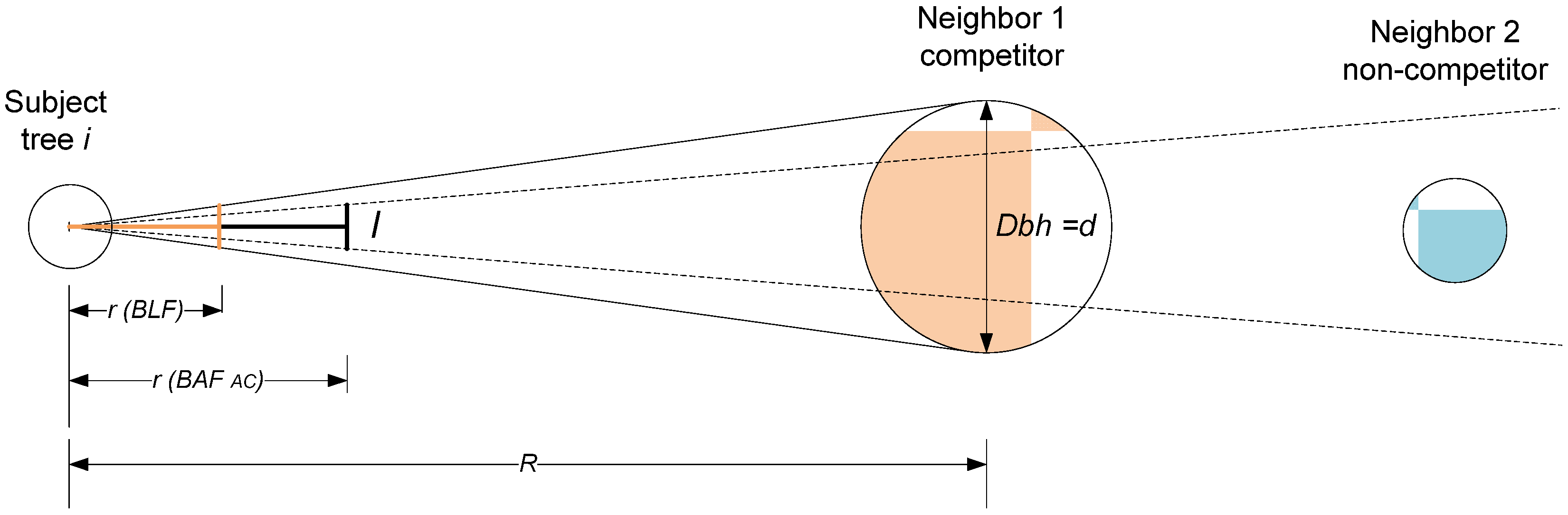
It has been suggested that the separate measurements of d and R could be omitted for determining the BLF by using the Wide Scale Relaskop or Telerelaskop to directly measure the subtended angle of the sample tree formed by the ratio d/R [11]. As displayed in Figure 1, it is possible to use a much simpler stick angle gauge to sight on a sample “in” tree to determine the BLF in forests of sparse understory. It should be possible to slide the crossarm or sighting intercept back to the point of r (BLF) so that the angle is coincident with the angle formed by diameter at breast height (Dbh) and distance R. It is then easy to devise a scale on the stick that directly furnishes the borderline factor of BLF or (d/R)²/4. Experience in southeastern United States, however, reveals that the Haglöf DME 201 ultrasonic distance measuring instrument is ideally suited for quickly measuring distances to the nearest 0.01 m without walking from the subject tree to the competing “in” tree. In forest conditions with dense understory vegetation consisting of shrubs and arborescents, the distance of many candidate trees that are further from the point center must be verified, since it is difficult to visually verify if the neighboring tree is included “in” the sample. The added time to measure the distance of close-to-point center trees is relatively small.

Numerous authors have discussed the demise of the use of permanent sample plots in forests of North America, based on an angle count (point sampling) estimator, for measuring forest stock and growth. Point sampling estimators have been considered appropriate for measuring growth, but this has been debated [13,14]. For example, the ubiquitous installation of permanent point sample plots in the 1960s and 1970s in North America was based on the low cost, ease of measurement, and efficiency of basal area and volume estimates. The disfavor of permanent point sample points became evident later when analyzing growth from remeasurements as additive or compatible estimates, such as those reported by Van Deusen et al. [15]. These estimates typically displayed high variance for the attribute of growth, while the efficient change estimator of Grosenbaugh was non-additive for biomass and/or volume (V₂ ≠ [V₁ + ΔV], where ∆ represents volume change and V_i is stand volume at time i [16]). Based on this evidence, Green [17] noted that it is difficult to detect much enthusiasm for the analysis of remeasurements using the angle count methodology.

Given the wide use of point sampling and the need to better quantify tree-level competition, this paper counters the arguments of Green [17] and explores the use of a new estimator and its properties in the estimation of basal area and volume growth from point sampling [18]. In addition, the prior estimator by McTague [18] can be decomposed on an individual tree basis to assign a competition index. Consequently, a comparison is made to the growth estimator using the traditional angle count constant for basal area factor (BAF_AC) created by Bitterlich [8], and the newer variable basal area factor (BAF_V) [18]. The primary research objectives of this analysis were to: (1) demonstrate the application of a new estimator for quantifying long-term production; (2) develop a new tree-level competition index based on point sampling; and (3) evaluate both estimators in two contrasting plantations and examine behavior of bias, precision, and additivity.

2. Materials and Methods

2.1. Plantation Locations and Tree Attributes

Two locations of loblolly pine (Pinus taeda L.) plantations were utilized to test the development of the BAF_V competition index. The first location was a 40 ha forest stand measured with a sampling intensity of one point (plot) per ha. The inclusion of “in” trees was determined with a BAF_AC = 4 using the same point location at ages 12 and 16. The population consists of 500 loblolly pine plantation trees in Santa Catarina, Brazil generated from the growth and yield model described by McTague [19]. The modeled population is derived from a thinned 12-year old stand, grown to age 16, with a site index, based on dominant height, of 20 m (base age 15). Parameters of the population generated from the growth and yield model are presented in

Table 1. Population parameters of thinned plantations of loblolly pine in Brazil and the United States used in this analysis.

Attribute	Measurement 1	Measurement 2	Change
Santa Catarina, Brazil
Total age (years)	12	16	4 years
Stem density (N)	500	500	0
Forest stand basal area (G; m2·ha−1)	28.8	39.1	10.3
Total green weight outside bark (W; t·ha−1)	195.2	335.5	140.3
Mean top height (H; m)	17.0	20.9	3.9
Quadratic mean diameter (dg; cm)	27.1	31.6	4.5
Weibull location (a) parameter	19.13	22.11	-
Weibull scale (b) parameter	8.709	10.257	-
Weibull shape (c) parameter	2.241	2.015	-
Southeastern United States
Total age (years)	17	-	-
Stem density (N)	330.5	-	-
Forest stand basal area (G; m2·ha−1)	14.13	-	-
Total green weight outside bark (W; t·ha−1)	100.0	-	-
Quadratic mean diameter (dg; cm)	23.3	-	-

Note: the 3-parameter Weibull cumulative density function is expressed as $F\left(x\right)=1-e^{-{\left(\frac{x-a}{b}\right)}^c}$, where x (x ≥ a) is the random variable representing tree diameter (d).

. Using prediction equations for the 10th and 63rd diameter percentiles of the growth model [19], Weibull parameters are recovered for the stand that are consistent with the stand-level estimate of basal area and the user-stipulated 500 trees per ha. Several parameter recovery methods for the Weibull distribution are presented in Burkhart and Tomé [12], including the use of diameter percentiles. In this case, each diameter class contains a proportion of 1/500 or 0.002 of the total trees, and the diameter class assignment is computed with the following formula by Clutter and Allison [20]:

$$d_i=a+b{\left[-\ln \left(1.001-0.002i\right)\right]}^{1/c}$$

(1)

where i = 1–500, d_i = diameter breast height of diameter class i, and a, b, and c, are Weibull distribution parameters.

Individual tree volume and green weight from the stump to the top of the tree were computed with the following equations presented in McTague [19].

$$v=0.0000289198d^{1.764357}{h}^{1.356831}$$

(2)

$$w=\frac{0.9672764v^{1.01834}}{{(d^{2}h)}^{0.004977}}$$

(3)

where

• v = total stem volume of a tree outside (including) bark in m³
• w = total stem green weight outside bark in tons
• d = individual tree diameter in cm determined at breast height of 1.3 m
• h = total tree height in m

The attributes of crown width and live crown ratio were predicted with equations localized for dominant trees of loblolly pine in Rio Grande do Sul and Santa Catarina, Brazil [21]. Crown size was used for computing an alternative competition index. The live crown ratio for individual trees was computed by adjusting the predicted live crown ratio by the ratio of individual tree height to Lorey height, while the predicted crown widths of dominant trees were adjusted with the ratio of diameter (d) to quadratic mean diameter (d_g).

Each of the 40 ha in the simulation at ages 12 and 16 contained the same population of 500 trees. The trees were randomly sorted for each ha and assigned once, at age 12, to grid coordinates. The spacing between rows was maintained at 2.5 m, while the distance between trees in the row was randomly perturbed. Since the simulated stand had been thinned with a combination of row and low thinning, every fourth row was completely removed. The simulation procedure was repeated 500 times using a 40 ha forest stand and a sampling intensity of one point (plot) per ha with multiple random starts within and between iterations. There was, however, no random perturbation associated with tree size. A small random perturbation, associated with the point (plot) location, was also simulated. The edge-effect and the potential bias associated with point locations close to mapped canopy openings or a forest edge were not investigated here as the point locations were at least 12.5 m away from the property boundary in this study.

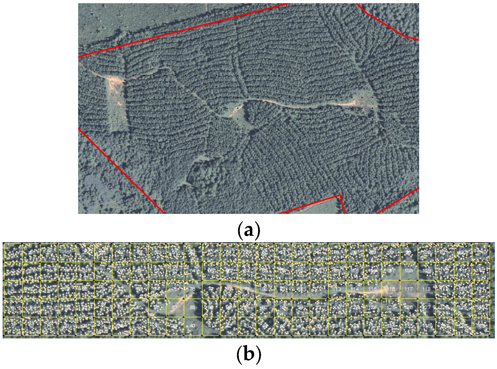
The second study site was located in a 17-year old loblolly pine plantation in the Piedmont physiographic region, Warren County, Georgia, USA. The 13.1 ha forest was completely stem-mapped following a thinning operation. The tract was divided into 135 quadrants with dimensions of 31.15 m × 31.15 m. All trees were tagged and had a measurement of d. Total tree heights were systematically measured on half of the stems in a quadrant. A common localized height-diameter equation was fit to the measured diameters (ds) and heights (hs) of each quadrant of the form: ln(h) = a₀ + a₁·(1/d), where a₀ and a₁ are estimated coefficients. Using the quadrant specific values of a₀ and a₁, trees without observed heights were then assigned a predicted height value.

Total stem green weight outside bark (w) in kg was estimated with the following equation from Harrison and Borders [22]:

$$w=0.049993d^{1.935455}{h}^{1.080621}$$

(4)

The attribute of crown width was estimated with coefficients specific for loblolly pine [23], while live crown ratio was predicted with the equation derived for loblolly pine in southeastern United States [24].

Remeasurements were not conducted for the southeastern United States plantation. However, the age 17 population parameters are provided in Table 1. Several salient features of the second study location are demonstrated in Figure 2, including the appearance of planting rows with considerable curvature and almost random direction. Large gaps in the forest canopy and non-planted openings were also visible, which leads inevitably to high variability and sampling error. Systematic sampling was conducted for the 13.1 ha forest stand using a sample size of 30 points (plots) with a BAF_AC = 4. The procedure was repeated 500 times using multiple random starts within and between iterations. For the sake of avoiding the placement of point (plot) locations too close to the long and narrow tract perimeter, there was no random perturbation of point centers from the multiple systematic grids. Point locations were at least 16 m away from the property boundary in this study location.

2.2. The Application of a New Estimator for Quantifying Long-Term Production

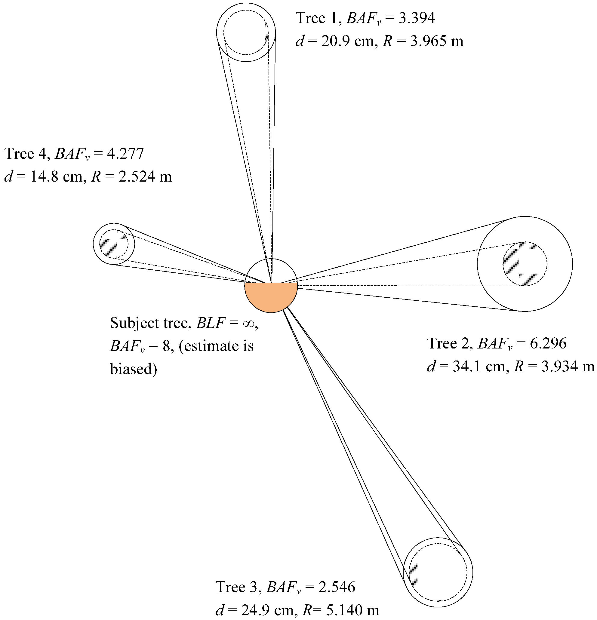
The proposed estimator will be demonstrated to be ideally suited for a system of permanent sample plots (PSPs) using a point sampling methodology for selecting “in” trees at each location. The point (plot) locations themselves are generally based on a probability based design. The change statistics in this study for attributes such basal area, volume, and stem density, were computed using only subject trees of the PSP points. These subject trees were selected by using the Bitterlich angle count basal area factor (BAF_AC).

The attributes assigned to subject trees were not computed with the constant BAF_AC. Rather, the estimator is a ratio that employs elements of both the Bitterlich angle count sample and the Spurr borderline factor, specifically (1−BAF_AC/BLF). The new variable basal area factor estimator (BAF_V) was presented by McTague [18] as:

$$G={\displaystyle \sum BA{F}_V}=2BA{F}_{AC}{\displaystyle \sum _{i=1}^m\left(1-\frac{BA{F}_{AC}}{BL{F}_i}\right)}$$

(5)

where

• m = the number of “in” trees at the point (plot)
• G = the basal area in m²·ha⁻¹
• BLF_i = the borderline factor for tree i, or (d_i/R_i)²/4
• d_i = diameter at 1.3 m (Dbh) in cm for tree i
• R_i = distance in m between the sample point and center of tree i
• BAF_AC = the Bitterlich angle count (point sampling) constant

Stem density, N, was estimated as $N={\displaystyle \sum _{i=1}^m\frac{BA{F}_V}{g_i}}$, where g_i is the individual tree basal area calculated as $k{d}_i^2\mathrm{with}k=\pi /40000$.

Basal area, and weight per ha, W, was predicted as $W={\displaystyle \sum _{i=1}^m\frac{BA{F}_V}{g_i}}{w}_i$ where w_i is individual tree green weight outside (including) bark. The basal area value for borderline “in” trees approaches zero, while trees close to the point center have a basal area approaching a value of 2 (BAF_AC) with the new estimator. Large trees have more influence on the attributes of basal area, stem density, and volume per ha. Estimates were computed by using the BAF_V and BAF_AC approaches for both the 16-year old plantation in Brazil and 17-year old plantation in USA in order to compare the results obtained by both methodologies. Yield and variance statistics of repeated sampling for the stand-level attributes of basal area (G), stem density (N), and green weight per ha (W) were computed from analysis-of-variance-type calculations of the between repetitions component.

2.3. Improved Compatible Estimator for Stand-Level Growth

The work of Hradetzky [25] was extended by McTague [26] whereby empirical comparisons of bias and precision among growth estimators from permanent point samples were presented. The problem of estimating growth from permanent point samples, as described by [25], consisted of varying sample composition from one measurement occasion to the next. Excluding the consideration of trees that died, or saplings that grew into merchantable size during the remeasurement interval, the sample plot on each remeasurement occasion would normally contain an augmented list of “in” trees. What differs among various point sampling growth estimators is the computation of the basal area and expansion factors for the new “in” trees at the time of remeasurement.

The original list of “in” trees is generally referred to as survivor trees, since they are measured “in” and are alive on both measurement occasions. Several authors preferred to allocate a basal area and expansion factor of zero to the new “in” trees [16,27]. Expanding upon the notation of Hradetzky [25], unbiased change estimators for green weight per ha of a pure panel design are presented below:

$$Z_{AC}={BAF}_{AC}\left[{\displaystyle \sum }_{i=1}^{m_2}\frac{w_{i2}}{g_{i2}}-{\displaystyle \sum }_{i=1}^{m_1}\frac{w_{i1}}{g_{i1}}\right]$$

(6)

where

• Z_AC = change in stand green weight (t·ha⁻¹) using the additive estimator [15] of angle count sampling
• w_ij = green weight for tree i at time j
• g_ij = individual tree basal area in m²·ha⁻¹ for tree i at time j
• m_j = number of sample “in” trees at a point (plot) at time j. The number of new “in” trees at the time of remeasurement equals (m₂ − m₁)

The most widely used estimator for computing change in biomass/volume from point samples is the non-additive Grosenbaugh estimator [16], which essentially ignores the contribution of the new “in” trees at the time of remeasurement into the calculation of growth:

$$Z_G={BAF}_{AC}\left[{\displaystyle \sum }_{i=1}^{m_1}\frac{\left(w_{i2}-w_{i1}\right)}{g_{i1}}\right]$$

(7)

where Z_G represents the change in green weight (t·ha⁻¹) using the non-additive Grosenbaugh estimator.

The change estimator by McTague [26] using BAF_V of Equation (5) is expressed as:

$$Z_V={\displaystyle \sum }_{i=1}^{m_2}{BAF}_V\frac{w_{i2}}{g_{i2}}-{\displaystyle \sum }_{i=1}^{m_1}{BAF}_V\frac{w_{i1}}{g_{i1}}$$

(8)

Since the BAF_V is very small for a new “in” tree at the time of remeasurement, the Z_V change estimator is very efficient, as virtually all the change is attributed to the growth of survivor trees. The equations for Z_AC, Z_G, and Z_V were used to compute the growth of stand-level green weight W. When w_ij was replaced with g_ij in Equations (6)–(8), stand-level growth of basal area G was computed.

2.4. Alternative Measures of Individual Tree Competition

Given that the estimator BAF_V was partially comprised of the borderline factor (BLF), it is only natural to believe that it is highly correlated with the Spurr point density index [7]. The Spurr point density competition index (CI_PD) requires that the (n) sample “in” trees be ordered by decreasing values of BLF_j, or (d_j/R_j)²/4, and it is expressed as:

$$C{I}_{PD}=\frac{{\sum }_{j=1}^n\left(j+0.5\right)BL{F}_j}{n}$$

(9)

The BAF_V also proves to be correlated to other distance-dependent indices. The Hegyi index (CI_H) [28], as applied by Daniels and Burkhart [29], was used in a point sampling context and it is a function of size of competing trees and distance:

$$C{I}_H={\displaystyle \sum }_{j=1}^n\left[\frac{\left(\frac{d_j}{d_i}\right)}{R_{ij}}\right]$$

(10)

where

• d_i = Dbh in cm of subject tree i
• d_j = Dbh in cm of competitor tree j
• R_ij = distance in m between subject tree i and competing tree j
• n = number of trees included “in” the sample for a given BAF_AC (excluding the subject tree)

One apparent drawback of both CI_PD and CI_H is the property that the indices predict values approaching infinity as R_ij becomes increasingly smaller. This is particularly problematic for stems that are forked below breast height (1.3 m) as the distance between subject tree i and competing tree j is often less than 0.5 m.

It is possible to demonstrate that the sample tree expansion factor (BAF_V/g) is also a function of tree size and distance (the expansion factor is used to compute the representative trees per ha of each sample tree of an angle count plot—this is unrelated to the linear expansion factor of Biging and Dobbertin [30] which is used as an adjustment for plot edge bias). Smaller trees of diameter (d) located near the angle count limiting distance, namely,$0.5d/\sqrt{BA{F}_{AC}}$, contribute less to stand weight than larger trees located near the sample point. It was hypothesized that the variable stand weight estimator, computed as the product of individual tree weight (w) and the expansion factor, might be correlated with the crown volume competition index [30]. The crown volume unweighted by distance (CVU) index was formed by projecting a 50° angle from the base of a subject tree and computing the crown volume of competing trees calculated at the point where the height angle intersects the tree bole axis. The crown is assumed to have a profile of a cone. The crown volume index is computed as:

$$CVU={\displaystyle \sum }_{i\ne j}^n\frac{C{V}_{aj}}{C{V}_i}$$

(11)

where

• CVU = unweighted crown volume index
• CVa_j = crown volume of competitor tree j above the point where the height angle cuts in height axis
• CV_i = crown volume of subject tree i
• n = number of trees included “in” the sample for a given BAF_AC

3. Results

3.1. Moving the Point Center from a Probability Based Location to the Center of The Subject Tree

The Z_V estimator makes it possible to assign a variable basal area factor to sample trees, based on size and distance, and efficiently estimate additive change or growth for a point or stand of interest. As demonstrated in Figure 3, when using a BAF_AC = 4, the sum of the BAF_V = 16.513 for the four competing trees. At each sample point, however, it is possible to further decompose the estimate of basal area and volume for the subject trees located “in” the sample and their respective competing trees. The methodology proposed here creates an absolute value of competition for the subject tree rather than a dimensionless competition index. A problem immediately surfaces, however, when attempting to quantify the contribution of basal area of the subject tree. Moving the point center from a probability based location to the center of the subject tree inflates the estimate of basal area for the subject tree and results in a bias. In other words, the BAF_V value for the subject tree must increase to the maximum value (2BAF_AC), resulting in a positive bias of stand basal area and volume.

It is possible to assign a value to the subject tree that achieves consistency between the basal area and volume per ha of the probability based design and the decomposition between subject and competitor trees. This implies assigning a BAF_V value to the subject tree that is less than 2(BAF_AC). The study described here attempts to quantify the new value assignment for the subject tree. The following steps are employed to compute the value for the subject tree. This new subject tree value, on average, is between the values of BAF_AC and 2(BAF_AC), and it should be assigned to each subject tree. It is computed with the sequence of steps below, and an example of the computations is provided in Appendix A.

(1)

A BAF_V competition index is computed for all competitor trees surrounding every subject tree at each sample point using Equation (5). Subject trees are temporarily assigned a competition index of zero.

(2)

The BAF_V competition index is summed by subject tree. An average BAF_V competition index is then computed at each sample point of the probability based location.

(3)

A difference is computed between the average variable basal area of the stand or strata (multiple sample points of the probability based design) and the average BAF_V competition index for the same sample points. This average difference is then assigned as the BAF_V competition index for each subject tree of the stand or strata.

The computation of the BAF_V competition index implies knowledge of the size and location of all trees in the neighborhood of each subject tree in the probability based design. The neighborhood in this case was defined by the angle count limiting distance, namely$0.5d/\sqrt{BA{F}_{AC}}$. Edge bias was avoided in Step 1 above since all neighboring trees of subject trees were measured, irrespective of whether they are contained in the original set of the “in” trees at the probability based sample point.

3.2. Sampling Simulation Statistics

Comparisons among the conventional (BAF_AC) and variable (BAF_V) estimators for the stand-level attributes of basal area, green weight, and stem density are presented in

Table 2. Estimates and efficiencies of the point sampling estimators obtained from repeated sampling using a BAF_AC = 4 for basal area, stem density, and green weight per ha.

Age, Location, andEstimator	Basal Area (G; m2·ha−1) $\sum \mathit{B}\mathit{A}\mathit{F}$		Stem Density (N) $\sum \mathit{B}\mathit{A}\mathit{F}\frac{1}{{\mathit{g}}_{\mathit{i}}}$		Green Weight (W; t·ha−1) $\sum \mathit{B}\mathit{A}\mathit{F}\frac{{\mathit{w}}_{\mathit{i}}}{{\mathit{g}}_{\mathit{i}}}$
	Mean	Variance of Mean	Mean	Variance of Mean	Mean	Variance of Mean
Age 16—Brazil
Conventional BAFAC	39.1	0.8	500.2	158	335.9	63
Equation (5) BAFV	39.2	0.6	500.7	98	336.2	45
Age 17—USA
Conventional BAFAC	14.0	1.7	357.8	779	109.3	63
Equation (5) BAFV	14.1	1.9	325.3	1027	99.5	107

Note: g_i is the individual tree basal area.

Clearly, the new BAF_V estimator was more efficient in the simulated forest plantation conditions of Brazil with more uniform occupancy of the growing space. On the other hand, the advantage of the BAF_V estimator for stand attributes in the United States plantation with large gaps was unclear, since it was slightly more accurate for green weight (W) and stem density (N), but less precise in terms of variance.

A real advantage of the BAF_V estimator appeared to be with permanent sample plots (PSP) and the measurement of growth. The statistical properties of growth (change) estimator, reported in

Table 3. Estimates and efficiencies of the point sampling change estimators obtained for basal area and green weight per ha in Brazil.

Estimator	Equation and Source	Change in Basal Area (ΔG; m2·ha−1)		Change in Green Weight (ΔW; t·ha−1)
		Mean	Variance of Mean	Mean	Variance of Mean
ZAC	Equation (6), [15]	10.3	0.81	140.0	52.9
ZG	Equation (7), [16]	10.3	0.10	140.5	16.8
ZV	Equation (8), [29]	10.3	0.18	140.3	13.4

Z_AC, change in stand green weight (t·ha⁻¹) using the additive estimator of angle count sampling; Z_G, the change in green weight (t·ha⁻¹) using the non-additive Grosenbaugh estimator; Z_V, change estimator using BAF_V.

, were of a repeatedly thinned plantation in Brazil and it excludes consideration of tree mortality or ingrowth (saplings) that grow into merchantable size during the remeasurement interval. Neither mortality nor ingrowth were considered as the components of growth that were responsible for the high variance of the additive (compatible) estimator. The high variance is normally attributed to the list of new “in” trees at the time of remeasurement. Since there was no change in the population value of stem density between ages 12 and 16 of the repeatedly thinned stand (see Table 1), no attempt was made to analyze the behavior of the change estimators for stem density. All estimators were accurate, but the BAF_V change estimator of Equation (8) was considerably more precise than the additive estimator which uses BAF_AC (Equation (6)).

Temporary plots based on angle count sampling (point sampling) are well known to be fast, easy, and inexpensive to install. The same is true for permanent sample plots based on angle count sampling, and if Equation (8) is used to measure change, it can be highly precise. It appeared that with little effort, all competitor trees surrounding the subject “in” trees can be measured with the BAF_V estimator for the purpose of building a competition index. If the BAF_AC for selecting the subject and competitor trees is larger than 3 m²·ha⁻¹, it should be possible to measure the size and distance of all the competitor trees, irrespective of whether they were included in or out of the probability based sample. Thus, mapping all the subject and competing trees is not onerous and there is no need to employ edge correction methods for competing trees outside the plot.

3.3. Correlation between BAF_V and Other Competition Indices

Table 4. Coefficients of partial determination for selected competition indices and the BAF_V and W estimators. The coefficient was defined as $r_{y3.12}^2=1-\frac{SSE\left(X_1,X_2,X_3\right)}{SSE\left(X_1,X_2\right)}$ , where SSE is the sum of squares of error, X₁ is a class variable denoting iteration, X₂ is a class variable denoting plot, and X₃ is either BAF_V or W. y denotes the dependent variable of CI_PD, CI_H, or CVU. The coefficient of partial determination between y and X₃, given that X₁ and X₂ are in the model is expressed as “$r_{y3.12}^2$”. SSE(X₁, X₂, X₃) is computed with the full model containing X₁, X₂, and X₃ as independent variables, while SSE(X₁, X₂) is the variation associated with the reduced model containing X₁, and X₂ as independent variables.

Country	Indices	Coefficient of Partial Determination (r2)
Brazil	BAFV and CIPD	0.718
	BAFV and CIH	0.582
	W and CVU	0.212
United States	BAFV and CIPD	0.903
	BAFV and CIH	0.724
	W and CVU	0.646

Note: CI_PD and CI_H are the Spurr point density and Hegyi competition indices respectively. CVU is the unweighted crown volume index. BAF_V and W are the proposed competition indices for basal area and weight.

presents the coefficient of partial determination (r²) between the BAF_V estimator, Spurr CI_PD, and Hegyi CI_H indices for plantations in Brazil and the United States using a BAF_AC = 4. The coefficient of partial determination (r²) was also reported for stand weight (W) and crown volume index of CVU. The simulated plantation conditions of Brazil have less plot to plot variability than the observed plot to plot variability in the United States. While the BAF_V and W estimators were more precise for the Brazilian conditions in estimating per ha attributes of basal area and stand green weight, they were less correlated to competition indices than the United States counterpart.

3.4. Assignment of an Unbiased BAF_V When the Subject Tree Is the Plot Center

As stipulated previously, the assignment of a competition index BAF_V = 2BAF_AC to each subject tree led to a positive bias. For the loblolly pine plantation in southern Brazil, a simulation procedure was used to compute an unbiased BAF_V value for all subject trees in the 12-year old, 40 ha forest. Although BAF_AC continued to be used to determine the count of the competing “in” trees, the appropriate subject tree BAF_V remained largely a function of BAF_AC. Recalling Step 3 from Section 3.1, a difference was computed between the average variable basal area of the stand of the probability based design, and the average BAF_V competition index for the same sample points of only the competing trees. This average difference was then applied to all subject trees of the stand or strata. An extension of this process was repeated for BAF_AC values ranging from 2 to 10 m²·ha⁻¹, as displayed in Figure 4.

Referring to Figure 4, and when BAF_AC = 4, the mean unbiased BAF_V for subject trees equaled 7.19 m²·ha⁻¹. The average subject tree BAF_V was not negative in any of the 500 repetitions, but it ranged from 5.47 to 9.11 m²·ha⁻¹.

For the loblolly pine plantation with stem-mapped trees in the Piedmont physiographic region of the United States, repeated sampling was used to compute the average unbiased value for subject tree BAF_V. Repeated sampling of 30 points (plots) with 500 repetitions and random starting locations was conducted for only the BAF_AC = 4. The analysis revealed that the average, unbiased BAF_V for the subject tree equaled 4.36 m²·ha⁻¹. The average subject tree BAF_V was not negative in any of the 500 repetitions, and it ranged from 1.26 to 7.14 m²·ha⁻¹.

4. Discussion

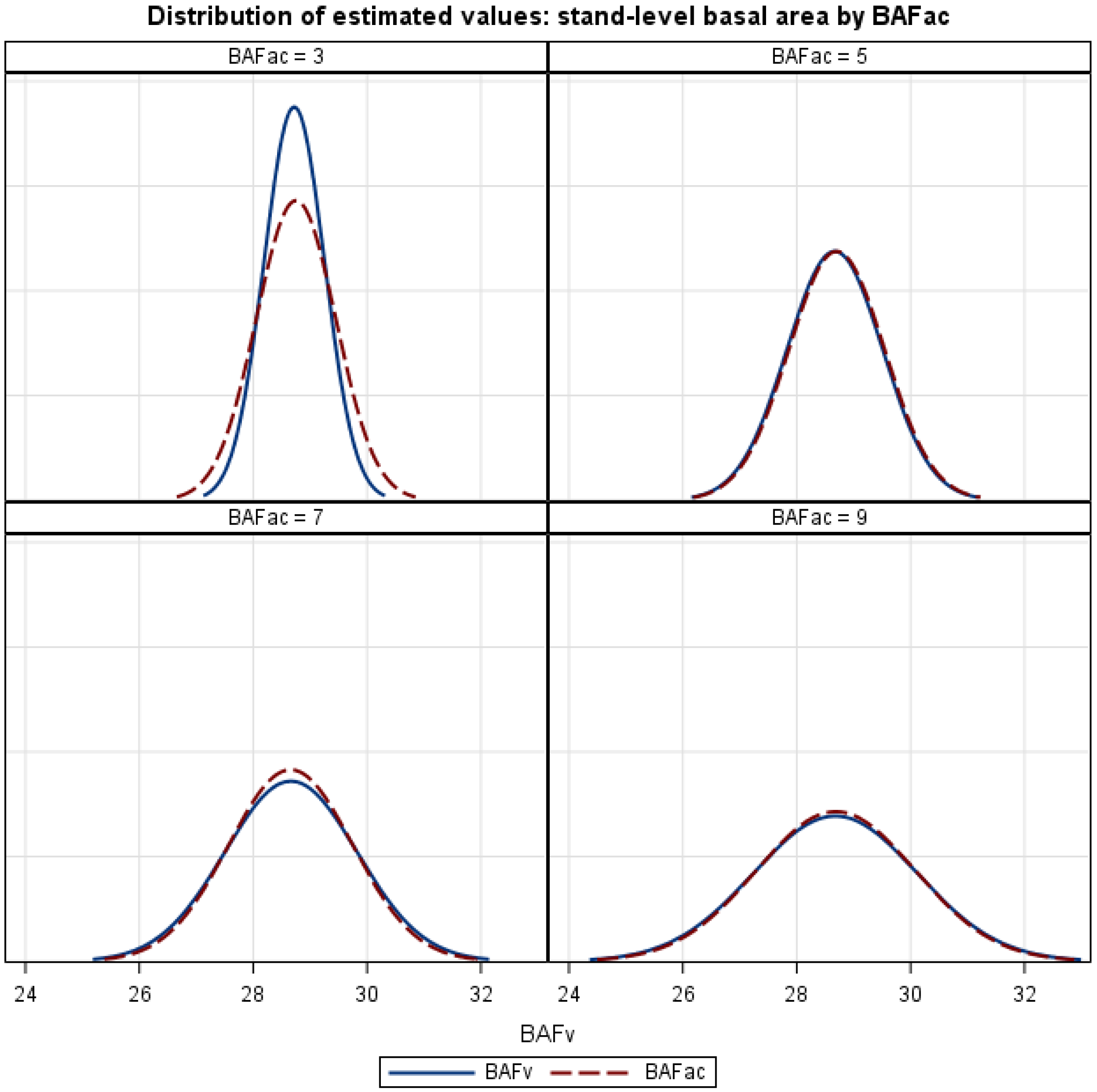
If tree diameter (d) and distance from the sample point to the subject “in” tree are measured during forest inventory, it is possible to compute the borderline factor (BLF) and the variable basal area factor BAF_V of Equation (5). As displayed in Figure 5, the BAF_V estimator is unbiased, implying that over many points, the expected values for the variable BAF estimator and the Bitterlich angle count estimator (∑BAF_AC) are identical. The BAF_V estimator also has desirable features, such as additivity and efficiency, when used for estimating change with permanent plots. The general consensus of the literature suggests that the Grosenbaugh growth estimator, Equation (7), is more efficient than the additive estimator, Equation (6), for most forest conditions and remeasurement intervals [25,31,32]. The drawback of the Grosenbaugh estimator is that it is non-additive (incompatible), so that volume (V₂ ≠ [V₁ + ΔV]). The disadvantage attributed to using the additive (compatible) Z_AC change estimator of Van Deusen et al. [15] is manifested in terms of high variance, which is normally attributed to the list of new “in” trees at the time of remeasurement [25]. The other alternatives, Z_G and Z_V, are superior in providing efficient change estimates for basal area and volume per ha. If the goal is to monitor forest growth, the variable and additive BAF estimator, Z_V, offers an attractive alternative to the common non-additive estimator of Z_G.

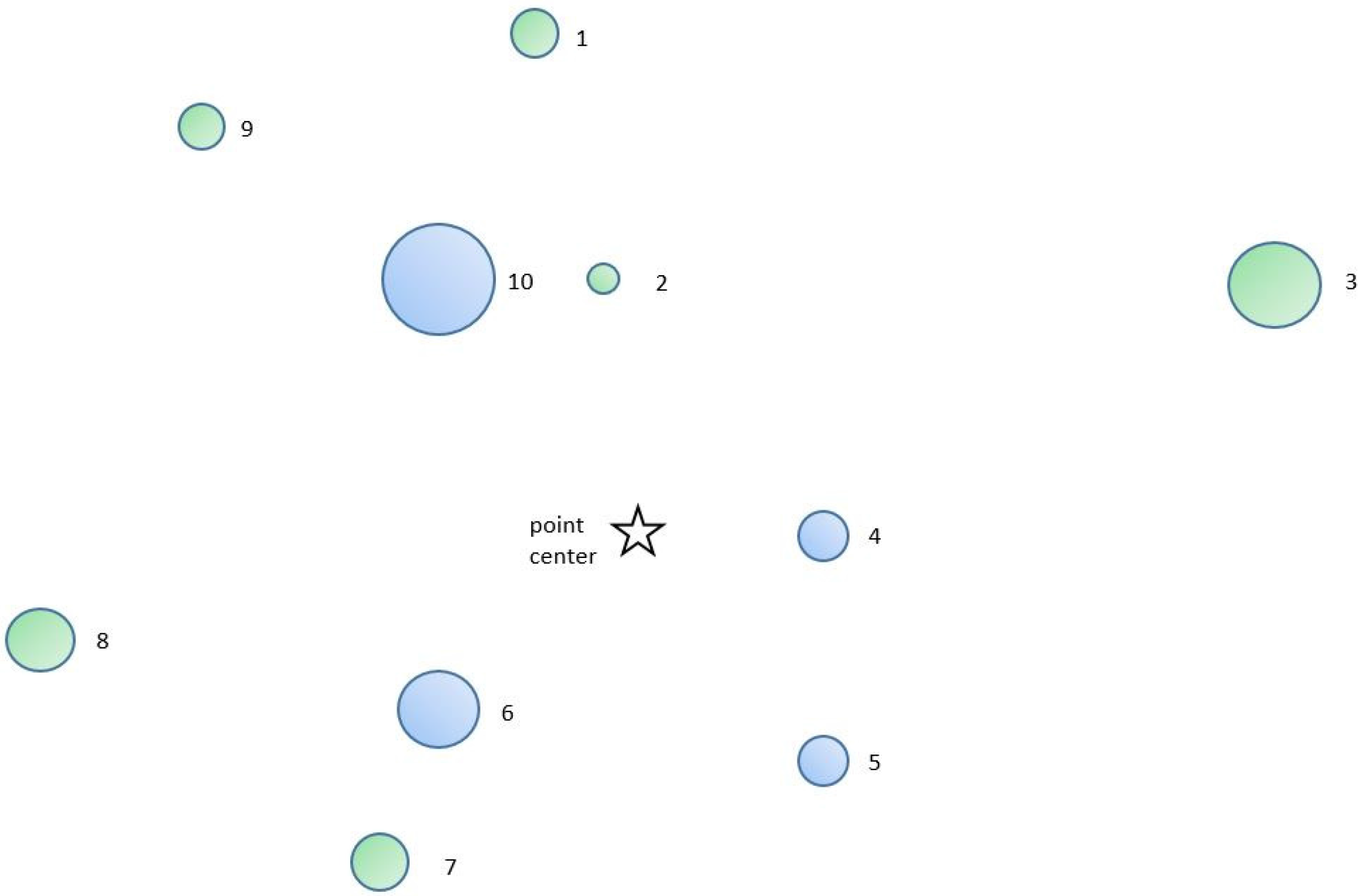
Quantifying the competition surrounding the subject tree with the BAF_V estimator was advantageous because the effect of size and distance of neighboring trees is reported in absolute units of m²·ha⁻¹ (or t ha⁻¹ in the case of green weight). Most competition indices, such as Hegyi, Equation (10), or the CVU, Equation (11), do not include the contribution of the subject tree in the competition computation, since the value of the subject tree equals infinity. Of course, this drawback is not true for the BAF_V estimator. In contrast, the contribution of the subject tree to the competition index based on BAF_V must be included if the sum of the individual competition values are to be additive with the stand level estimate of basal area or volume.

Following the establishment of the permanent sample plots (points), neighboring competitor trees that are centered around each subject tree can also be measured. As a practical matter, a BAF_AC < 3 m²·ha⁻¹ is not recommended. It was desirable to keep the total sample size of subject and competing trees manageable by using a BAF_AC ≥ 3. One recent investigation arrived at the conclusion that the Bitterlich angle count method was not the best method for selecting competitor trees [6]. Here, we contend that Bitterlich method should not be used exclusively for just selecting competitor trees, but rather the point sampling expansion factors should also be employed to scaling the competition indices up to a per ha level. If the expansion factor of (BAF_V/g) is used, the competition indices are both spatially explicit and can express the competition in absolute values at a per ha level.

A drawback of the BAF_V estimator for measuring competition is that it is biased for measuring the competition contribution of the subject tree. This paper presents a methodology for arriving at a stand level value for BAF_V for the subject tree that removed the bias. The proposed method then assigns the same BAF_V value to all subject trees over all points (plots) in the stand. Compatibility or additivity is achieved at the stand level, but not at the point or plot level. Compatibility is mathematically possible at the point (plot) level, however, it may result in either the negative assignment of BAF_V for the subject tree, or the need to adjust the values of both subject and competing trees. Clearly, the drawbacks of achieving compatibility at the point (plot) level outweigh the possible benefits.

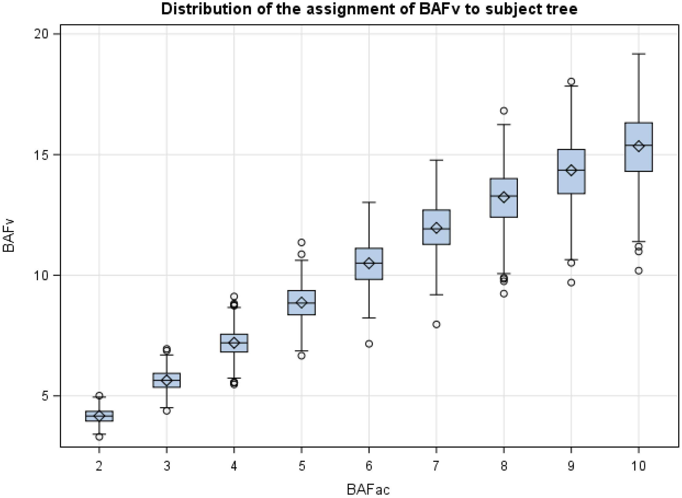
One puzzling outcome of this study was the difference of 2.83 m²·ha⁻¹ (7.19 m²·ha⁻¹ vs. 4.36 m²·ha⁻¹) between the assignment of the average unbiased BAF_V value for the subject tree, using a BAF_AC = 4, when comparing southeastern United States and Brazil. Clearly the variability in the simulated Brazilian plantation was less pronounced than the observed conditions in southeastern United States, with large holes in the forest canopy and frequent null tallies at some points (plots) in the latter. In hindsight, the study would have benefited from a larger stem-mapped forest in the United States, or with a more equal distribution of forest canopy holes between the center and periphery of the stand. Without question, the assignment of 2(BAF_AC) to each subject tree results in a positive bias, irrespective of the forest structure and conditions.

The additive competition indices proposed here are well suited for growth and yield studies that rely on PSPs, where it is imperative that change statistics are estimated efficiently. In this case, the BAF_V estimator is perfectly suited for measuring growth. In addition, it is well known that angle count samples are inexpensive to install and maintain. With a selection of a BAF_AC ≥ 3, it should be physically and economically feasible to measure all competitor trees and obviate the requirement for edge correction. A difficulty can arise, however, when using a BAF_AC ≥ 3, if the forest is subjected to intermediate harvests that involve strips or mechanical row thinning. Depending on the width of the harvest cut, a large proportion of the subject and competing trees of the point can be eliminated, compromising the utility of the remeasured plot over the next measurement interval. This is particularly true for forest stands where the quadratic mean diameter (d_g) is less than 15 cm and the equivalent plot size is rather small. As trees grow larger in size and the effective plot size increases, the abrupt change in sample size associated with cutting diminishes.

5. Conclusions

Competition indices are important components of forest growth and yield models and also help guide silvicultural decisions. Most spatially-explicit competition indices are suited to large, fixed-area plots. Here, a modified competition index suitable for variable-radius plots, first proposed by Spurr, was developed and tested. Based on data from two loblolly pine plantations, the new index showed high correlation with other commonly used spatially-explicit competition indices, but has other desirable properties when compared to these other indices. In particular, the index developed in this analysis eliminates the need for edge correction methods and ensures compatibility with stand-level estimates of basal area and stem density. Overall, given the simplicity and ease of measurement as well as the computation of this index, the extension to other forest types is suggested.

References

1. Weiskittel, A.R.; Hann, D.W.; Kershaw, J.A., Jr.; Vanclay, J.K. Forest Growth and Yield Modeling; John Wiley & Sons: Chichester, UK, 2011. [Google Scholar]
2. Pretzsch, H. Forest Dynamics, Growth and Yield: From Measurement to Model; Springer: Berlin, Germany, 2009. [Google Scholar]
3. Daniels, R.F. Notes: Simple competition indices and their correlation with annual loblolly pine tree growth. For. Sci. 1976, 22, 454–456. [Google Scholar]
4. Pedersen, R.Ø.; Nӕsset, E.; Gobakken, T.; Bollandsås, O.M. On the evaluation of competition indices—The problem of overlapping samples. For. Ecol. Manag. 2013, 310, 120–133. [Google Scholar] [CrossRef]
5. Soares, P.; Tomé, M. Distance-dependent competition measures for eucalyptus plantations in Portugal. Ann. For. Sci. 1999, 5, 307–319. [Google Scholar] [CrossRef]
6. Maleki, K.; Kiviste, A.; Korjus, H. Analysis of individual tree competition effect on diameter growth of silver birch in Estonia. For. Syst. 2015, 24, e023. [Google Scholar]
7. Spurr, S.H. A measure of point density. For. Sci. 1962, 8, 85–96. [Google Scholar]
8. Bitterlich, W. Die Winkelzählprobe. Allem. For. Holzwirtsch. Ztg. 1948, 59, 4–5. [Google Scholar] [CrossRef]
9. Tomé, M.; Burkhart, H.E. Distance-dependent competition measures for predicting growth of individual trees. For. Sci. 1989, 35, 816–831. [Google Scholar]
10. Rouvinen, S.; Kuuluvainen, T. Structure and asymmetry of tree crowns in relation to local competition in a natural mature Scots pine forest. Can. J. For. Res. 1997, 27, 890–902. [Google Scholar] [CrossRef]
11. Bitterlich, W. The Relascope Idea: Relative Measurements in Forestry; Commonwealth Agricultural Bureaux: Farnham Royal, UK, 1984. [Google Scholar]
12. Burkhart, H.E.; Tomé, M. Modeling Forest Trees and Stands; Springer: Dordrecht, The Netherlands, 2012. [Google Scholar]
13. Husch, B.; Miller, C.I.; Beers, T.W. Forest Mensuration, 3rd ed.; John Wiley & Sons: New York, NY, USA, 1982. [Google Scholar]
14. Furnival, G. Forest sampling—Past performance and future expectations. In Forest Resource Inventories Workshop Proceedings; Frayer, W.E., Ed.; Colorado State University: Fort Collins, CO, USA, 1979; Volume 1, pp. 320–326. [Google Scholar]
15. Van Deusen, P.C.; Dell, T.R.; Thomas, C.E. Volume growth estimation for permanent horizontal points. For. Sci. 1986, 32, 415–422. [Google Scholar]
16. Grosenbaugh, L.R. Point-Sampling and Line-Sampling: Probability Theory, Geometric Implications, Synthesis; USDA Forest Service, Southern Forest Experiment Station: New Orleans, LA, USA, 1958.
17. Green, E.J. Forest growth with point sampling data. Conserv. Biol. 1992, 6, 296–297. [Google Scholar] [CrossRef]
18. McTague, J.P. New and composite point sampling estimates. Can. J. For. Res. 2010, 40, 2234–2242. [Google Scholar] [CrossRef]
19. McTague, J.P.; Bailey, R.L. Compatible basal area and diameter distribution models for thinned loblolly pine plantations in Santa Catarina, Brazil. For. Sci. 1987, 33, 43–51. [Google Scholar]
20. Clutter, J.L.; Allison, B.J. A growth and yield model for Pinus radiata in New Zealand. In Growth Models for Tree and Stand Simulation; Fries, J., Ed.; Research Note No. 30; Royal College of Forestry, Department of Forest Yield Research: Stockholm, Sweden, 1974; pp. 136–170. [Google Scholar]
21. Padoin, V.; Finger, C.A.G. Relações entre as dimensões da copa e a altura das árvores dominantes em povoamentos de Pinus taeda L. Ciênc. Florest. 2010, 20, 95–100. [Google Scholar] [CrossRef]
22. Harrison, W.M.; Borders, B.E. Yield Prediction and Growth Projection for Site-Prepared Loblolly Pine Plantations in the Carolinas, Georgia, Alabama, and Florida; PMRC Technical Report. 1996-1; Warnell School of Forest Resources, Plantation Management Research Cooperative, University of Georgia: Athens, GA, USA, 1996. [Google Scholar]
23. Bechtold, W.A. Crown-diameter prediction models for 87 species of stand-grown trees in the eastern United States. South. J. Appl. For. 2003, 27, 269–278. [Google Scholar]
24. Dyer, M.E.; Burkhart, H.E. Compatible crown ratio and crown height models. Can. J. For. Res. 1987, 17, 572–574. [Google Scholar] [CrossRef]
25. Hradetzky, J. Concerning the precision of growth estimation using permanent horizontal point samples. For. Ecol. Manag. 1995, 71, 203–210. [Google Scholar] [CrossRef]
26. McTague, J.P. The use of composite estimators for estimating forest biomass and growth from permanent sample plots established by the angle count method. In Proceedings of the 2013 Joint Statistical Meetings, Montréal, QC, Canada, 3–8 August 2013; American Statistical Association: Washington, DC, USA, 2015; pp. 4663–4677. [Google Scholar]
27. Beers, T.W.; Miller, C.I. Point Sampling: Research Results Theory and Applications; Purdue University Agricultural Experiment Station: Lafayette, IN, USA, 1964; No. 786. [Google Scholar]
28. Hegyi, F. A simulation model for managing Jack-pine stands. In Growth Models for Tree and Stand Simulation; Fries, J., Ed.; Research Note No. 30; Royal College of Forestry, Department of Forest Yield Research: Stockholm, Sweden, 1974; pp. 74–90. [Google Scholar]
29. Daniels, R.F.; Burkhart, H.E. Simulation of Individual Tree Growth and Stand Development in Managed Loblolly Pine Plantations; Publication No. FWS-5-75; Division of Forestry and Wildlife Resources, Virginia Polytechnic Institute and State University: Blacksburg, VA, USA, 1975.
30. Biging, G.S.; Dobbertin, M. A comparison of distance-dependent competition measures for height and basal area growth of individual conifer trees. For. Sci. 1992, 38, 695–720. [Google Scholar]
31. Gregoire, T.G. Estimation of forest growth from successive surveys. For. Ecol. Manag. 1993, 56, 267–278. [Google Scholar] [CrossRef]
32. Thérien, G. Relative efficiency of point sampling change estimators. Math. Comput. For. Nat. Res. Sci. 2011, 3, 64–72. [Google Scholar]
Figure 1. An angle stick gauge of a predetermined length r (BAFAC) from the peep sight and a crossarm of predetermined width l is used to determine the sample size of neighbors in the competition index for the subject tree. Neighbor 1 is a competitor tree because it subtends an angle that is larger the critical angle defined by the basal area factor of angle count sampling (BAFAC). Conversely, Neighbor 2 is not included in the sample and is considered a non-competitor. BAFAC, angle count basal area factor; BLF, borderline factor or (d/R)2/4. (Adapted from [12].)
Forests 07 00238 g001
Figure 2. Aerial images for the Southeastern United States study site. Panel (a) displays a recently thinned, 17-year old plantation, containing planting rows with curvature and numerous switches in planting direction; Panel (b) is the 13.1 ha rectangle from the center of the stand and contains 135 quadrants with dimensions of 31.15 × 31.15 m. Individual trees were mapped and depicted with white dots.
Forests 07 00238 g002
Figure 3. Conceptual figure demonstrating calculations of new estimator. Each competing tree is assigned a variable basal area factor (BAFV) depending upon its size and distance to the subject tree.
Forests 07 00238 g003
Figure 4. Box plot of the subject tree variable basal area factor (BAFV) and the traditional angle count factor (BAFAC) for a loblolly pine plantation in Brazil. Each open diamond symbol represents the average value of 500 iterations.
Forests 07 00238 g004
Figure 5. Employing the example from Brazil, the population value of the stand at age 12 for total basal area (G; m2·ha−1) is equal to 28.8. Both estimators, namely BAFAC and BAFV, are unbiased for any basal area factor, however, the BAFV estimator is somewhat more precise when BAFAC < 4.
Forests 07 00238 g005