Article

Effects of Temporal and Interspecific Variation of Specific Leaf Area on Leaf Area Index Estimation of Temperate Broadleaved Forests in Korea

1
Department of Forest Resources, Kangwon National University, Chuncheon 200-701, Korea
2
Department of Forest Sciences, Seoul National University, Seoul 151-921, Korea
3
Research Institute for Agriculture and Life Sciences, Seoul National University, Seoul 151-921, Korea
4
Interdisciplinary Program in Agricultural and Forest Meteorology, Seoul National University, Seoul 151-744, Korea
5
National Center for AgroMeteorology, Seoul National University, Seoul 151-744, Korea
*
Authors to whom correspondence should be addressed.
Forests 2016, 7(10), 215; https://doi.org/10.3390/f7100215
Submission received: 12 June 2016 / Revised: 8 September 2016 / Accepted: 21 September 2016 / Published: 28 September 2016

Abstract

:
This study investigated the effects of interspecific and temporal variation of specific leaf area (SLA, cm2·g−1) on leaf area index (LAI) estimation for three deciduous broadleaved forests (Gwangneung (GN), Taehwa (TH), and Gariwang (GRW)) in Korea with varying ages and composition of tree species. In fall of 2014, fallen leaves were periodically collected using litter traps and classified by species. LAI was estimated by obtaining SLAs using four calculation methods (A: including both interspecific and temporal variation in SLA; B: species specific mean SLA; C: period-specific mean SLA; and D: overall mean), then multiplying the SLAs by the amount of leaves. SLA varied across different species in all plots, and SLAs of upper canopy species were less than those of lower canopy species. The LAIs calculated using method A, the reference method, were GN 6.09, TH 5.42, and GRW 4.33. LAIs calculated using method B showed a difference of up to 3% from the LAI of method A, but LAIs calculated using methods C and D were overestimated. Therefore, species specific SLA must be considered for precise LAI estimation for broadleaved forests that include multiple species.

1. Introduction

The total leaf area, where a substantial proportion of metabolic activities of forest ecosystem occur, determines the productivity of a forest [1,2,3,4]. Moreover, leaf area is an important factor in regulating the circulation of carbon, water, and energy between the atmosphere and the biosphere, as it influences the amount of light, wind, and water that flow in and out of the forest ecosystem [5,6,7].
The amount of leaves in a forest ecosystem can be quantified by the leaf area index (LAI), which is defined as the sum of total leaf areas per unit of ground area. However, in the case of broad-leaved trees, it is generally defined as the sum of one side of leaf area per unit of ground area [8].
LAI can be estimated by direct or indirect methods. The most common direct methods include harvesting all leaves, but this is destructive and unsustainable; allometric equations derived from harvested trees’ diameter at breast height (DBH) and tree height, or collecting fallen leaves with litter traps are the most commonly used direct methods [5,9,10,11,12,13,14]. Indirect methods include optical devices (e.g., digital cameras, LED (Light Emitting Diode) sensors, and LAI-2200C (a canopy analyzer)), or various vegetation indices estimated from satellite images, such as MODIS(Moderate- resolution Imaging Spectroradiometer) [10,13].
Indirect methods have been used in many studies due to their improving accuracy, and they make it easier and faster to estimate LAI compared to direct methods [2,12]. However, it is essential to compare indirect and direct methods [15,16,17,18], since it is common to underestimate the amount of leaves in a dense canopy or overestimate when the leaf area is small [10,19]. In particular, the litter trap method is more widely used in forests with deciduous trees than in forests with evergreen trees because it allows repeated measurements over many years and seasonal observations [5,20]. In stands or smaller scale experiments, such as free air CO2 enrichment systems or open top chambers, direct methods using fallen leaves are primarily used for LAI measurement [21,22].
LAI estimation by collecting fallen leaves is calculated by multiplying the dry weight of fallen leaves by the specific leaf area (SLA), providing the leaf area per unit dry weight. SLA differs with tree species, and even the same species show SLA variations depending on environmental conditions, such as soil fertility and dryness. Even within an individual tree crown, SLA varies depending on the light environment of the leaves [5,23,24]. In addition, the size and the weight of a leaf changes as it unfolds, withers, and falls, and even the same fallen leaf varies in SLA depending on the extent of nutrient remobilization according to the time of its fall, such as in early defoliation due to disturbance (e.g., typhoon, flood, drought). Therefore, temporal, spatial, and interspecific variations in SLA should be carefully considered [9,13,25]. However, despite its importance, little research has investigated these SLA effects on LAI. In particular, since it takes time and effort to estimate SLA for individual tree species, research has usually been conducted in pure forests (consisting of a single tree species) rather than mixed broadleaved forests, where various tree species coexist [6,9,26].
As the biome most influenced by human interference and destruction, temperate broadleaved forests located in central and Eastern Europe, East Asia, and Northeast America have a high level of ecological significance [27]. However, most are natural broadleaved forests, with many tree species growing in a single stand, which is inconvenient for estimating SLA for individual tree species. Hence, very little research on the influence of interspecific, temporal, and regional variations in SLA on LAI has been conducted. This study (1) measured interspecific and temporal SLA of fallen leaves in three representative natural broadleaved forests in Korea that are in different succession stages; (2) estimated LAI using four estimation methods explicitly considering SLA variation; and (3) compared the methods to determine how to estimate precise LAI quickly and efficiently.

2. Materials and Methods

2.1. Site Description

Plots of 20 m × 20 m were established in three deciduous broadleaved forests. Two of the forests were representative climax forests of South Korea as a result of artificial conservation for hundreds of years due to royal tombs of the Joseon Dynasty being located in the forests (Gwangneung Arboretum (GN) in the city of Pocheon in Gyeonggi province), and low accessibility (Mt. Gariwangsan (GRW) in the city of Pyeongchang in Gangwon province) (Table 1). The third forest was Mt. Taehwa (TH), Seoul National University’s research forest, generated in the 1960s near the city of Gwangju. GN and TH plots were protected from wind due to their location in the mountain hillside, but the GRW plot was exposed to wind due to its location on a mountain top. All three research sites were located near existing flux towers, so meteorological data were available at 30 min intervals. The average temperature of the GRW growing season (16 May–20 November 2014) was 13.0 °C, which was lower than GN 17.7 °C (annual average temperature for 2014 = 11.1 °C) and TH at 18.1 °C (annual average temperature for 2014 = 11.4 °C) for the same period. Total precipitation during the same period was 573.0 mm for GN (annual total precipitation for 2014 = 763.0 mm), 531.1 mm for TH (annual total precipitation for 2014 = 791.5 mm), and 871.57 mm for GRW [19,28,29,30].
Dominant species in the upper canopy of each plot were as follows: Quercus serrata and Carpinus laxiflora in the GN plot; Q. serrata and Quercus aliena in the TH plot; and Fraxinus rhynchopylla, Kalopanax septemlobus, and Sorbus alnifolia in the GRW plot. The basal areas of upper-canopy tree species for GN, TH, and GRW were 90.5%, 83.0%, and 80.8% of total basal area, respectively; and the significance values, estimated by totaling relative density, relative frequency, and relative cover degree, were 47.4%, 54.7%, and 52.0% of their respective totals.

2.2. Leaf-Litter Collection and SLA Measurements
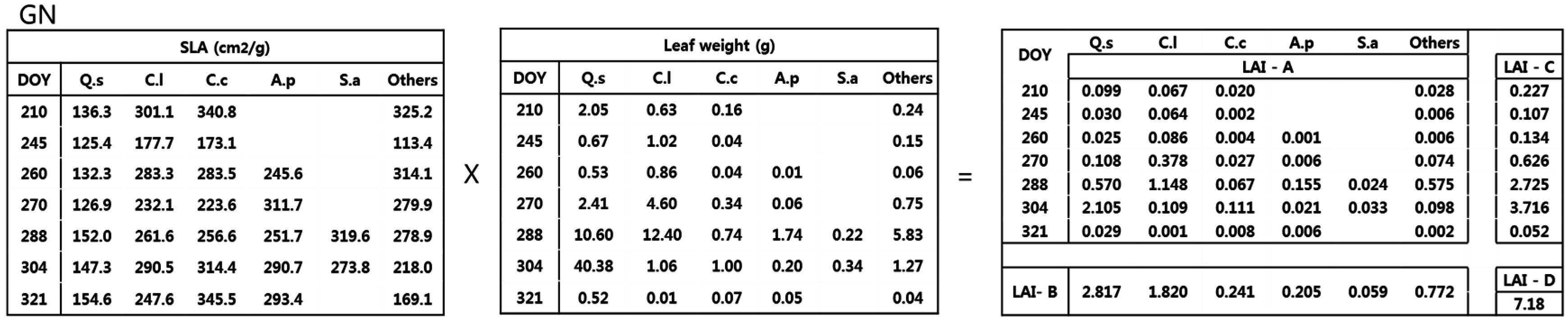
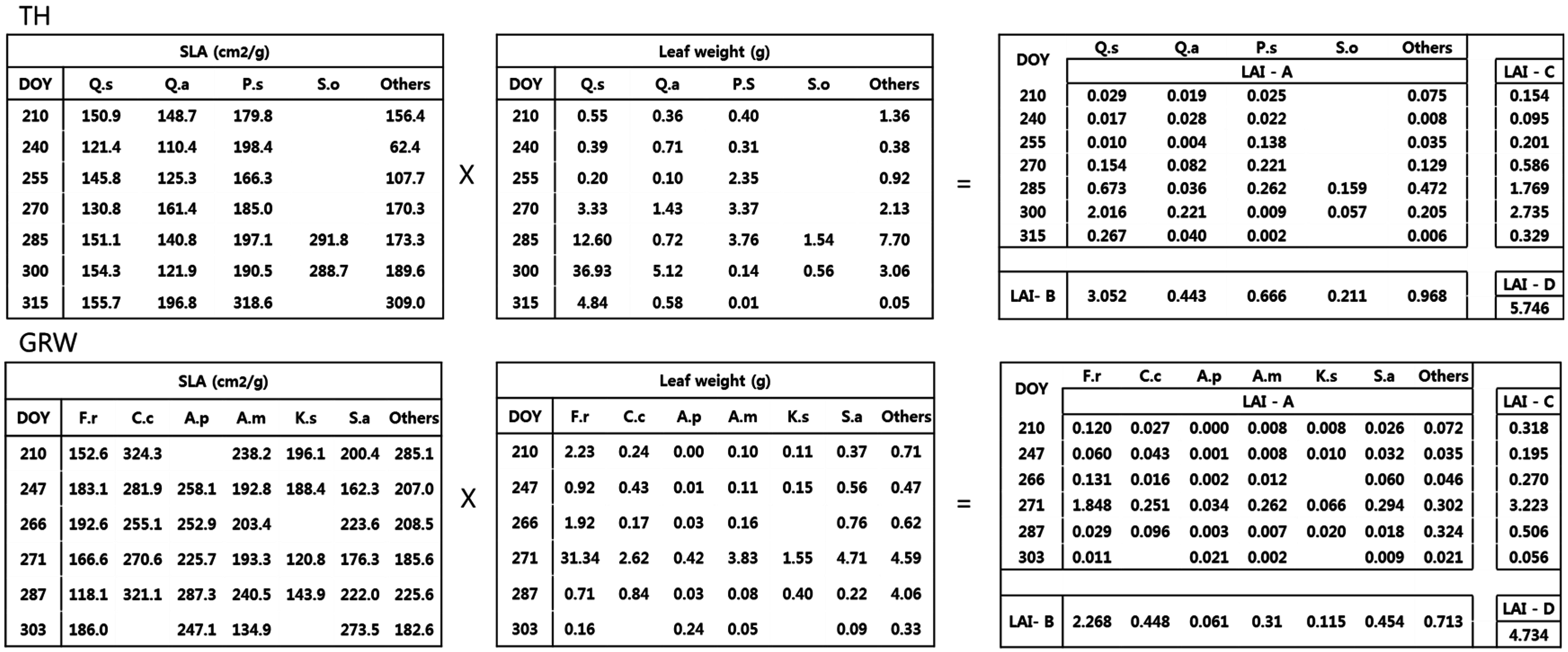
Fallen leaves were collected using five circular litter-traps (60 cm inlet diameter; 60 cm height) installed randomly in each plot. Leaf collection started in early August 2014, and leaves were collected once for the month of August, in which the amount of fallen leaves was small, and at approximately 15-day intervals for September through the end of November. Collection was conducted six times at GRW, which has a shorter growing season than the two other areas, and seven times for GN and TH. Collected leaves were classified by major tree species of each plot, and whether the number of leaves with full shape was low (40 or less). After excluding torn and damaged leaves, a complete enumeration survey was conducted. In cases where the number of leaves was sufficiently high, five or more sample leaves were taken from each trap.
Leaf area was measured using the LIA 32 ver.0.377e program (Kazukiyo Yamamoto, Nagoya University, Japan) after the leaves were recovered to the original shape and size by soaking and spreading them in water. The area measured leaves were dried in a drying oven (VTR-115, Isuzu, Japan) at 65 °C for more than two days, then SLA (cm2·g−1) was calculated by dividing leaf area by dry weight. The remaining leaves were dried immediately after classification, and the dry weight of each species was measured.

2.3. LAI Estimation

LAI was calculated by dividing the product of SLA (cm2·g−1) and dry weight (g) of leaves by the trap area (cm2). Four different LAI values were obtained using different representative SLA values (Figure 1):
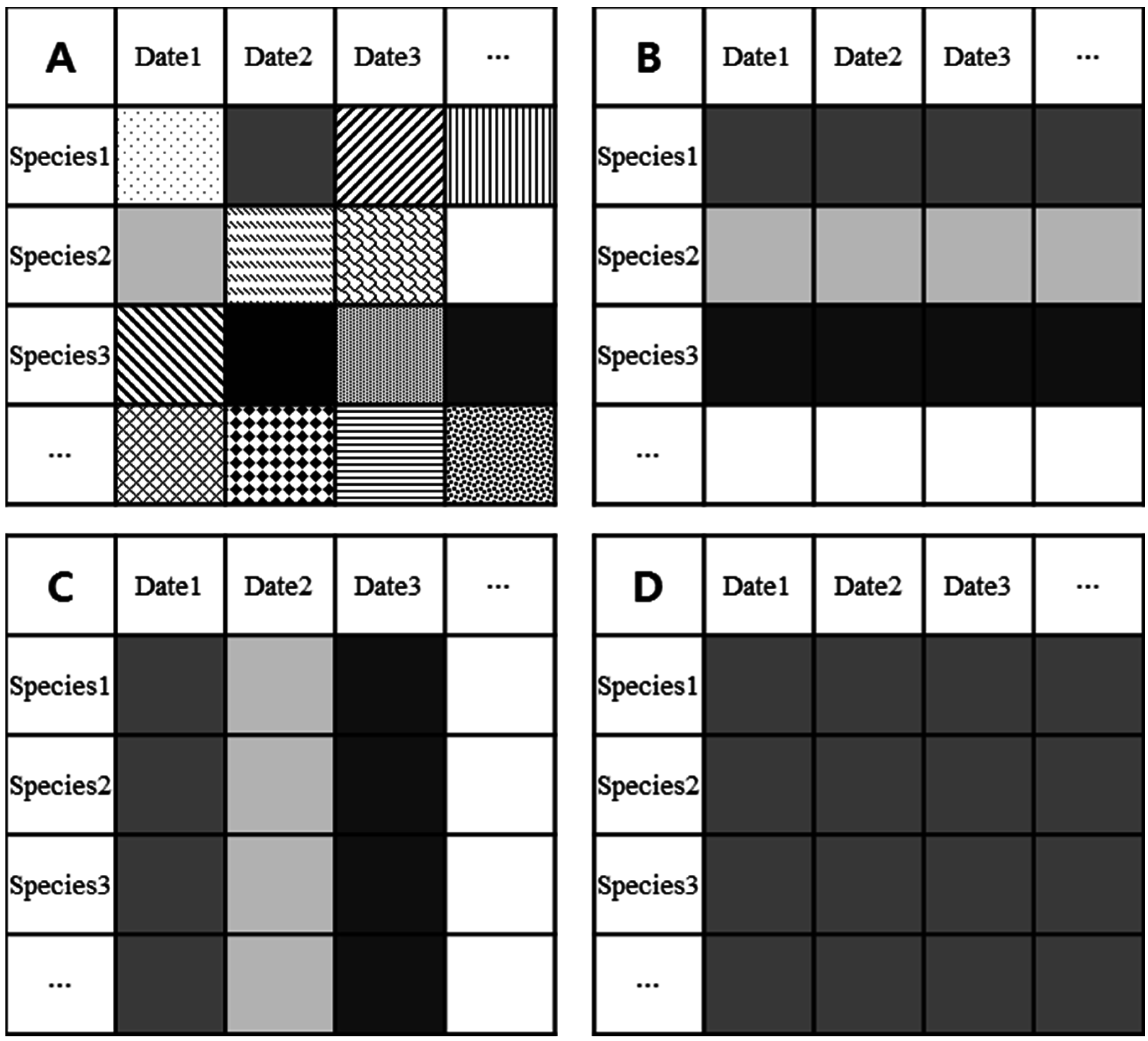
  • Method A used the species specific SLA and dry weight from each collection date. This is considered as the true or reference LAI since it accounted for species and temporal variations.
  • Method B used the average species specific SLA from all collection dates and the total dry weight of each species, ignoring seasonal variation.
  • Method C used the average period specific SLA, ignoring interspecific variation, and the total dry weight of each period.
  • Method D used the average SLA, ignoring temporal and interspecific variation, and the total dry weight of all species.
The maximum LAI of each study area was calculated by summing the LAIs from the four methods.

2.4. Statistical Analysis

Differences in average SLAs for individual species and periods of each study site were tested using analysis of variance (ANOVA). Where a difference was significant, a post hoc test was conducted (Duncan’s test). Differences in maximum LAI between method A and method B, C, or D were tested for statistical significance using a paired t-test of five litter traps. All statistical analyses were performed using SPSS Version 22 (IBM Inc., New York, NY, USA, 2012).

3. Results

3.1. Temporal and Interspecific SLA Variation

In all plots, SLAs for individual species, collection dates, and species by collection period showed significant differences (Table 2). Table 3 shows species and period specific SLA for GN, TH, and GRW. In GN, SLA increased in the order: Q. serrata, C. laxiflora, Acer pseudosieboldianum, Carpinus cordata, and S. alnifolia, whereas the order in TH was Q. aliena, Q. serrata, Prunus sargentii, and Styrax obassia. In GRW, SLAs increased in the order of K. septemlobus, F. rhynchophylla, S. alnifolia, Acer mono, A. pseudosieboldianum, and C. cordata. In all plots, SLAs of upper canopy species (Q. serrata, C. laxiflora, Q. aliena, P. sargentii, F. rhynchophylla, and K. septemlobus) were lower than those of lower canopy species (C. cordata, A. pseudosieboldianum, and S. obassia).
SLAs were lowest in mid-September, with 161.4 cm2·g−1 and 149.4 cm2·g−1 in GN and TH, respectively, and 182.6 cm2·g−1 in mid-November in GRW. Species that showed temporal SLA variation were Q. serrata, C. cordata, and S. alnifolia in GN, Q. aliena and S. obassia in TH, and all species except A. mono in GRW. In contrast, C. cordata in GN, Q. serrata and P. sargentii in TH, and A. mono in GRW showed no significant temporal variation (p > 0.05). Due to various reactions of SLAs among different species with time, interaction effects between species and collection dates were significant in all plots (Table 2). SLAs averaged for individual plots, ignoring species and collection dates, were in the following order: TH, 169.3 cm2·g−1 (n = 752); GRW, 201.6 cm2·g−1 (n = 894); and GN, 222.8 cm2·g−1 (n = 917) (p-value < 0.001).

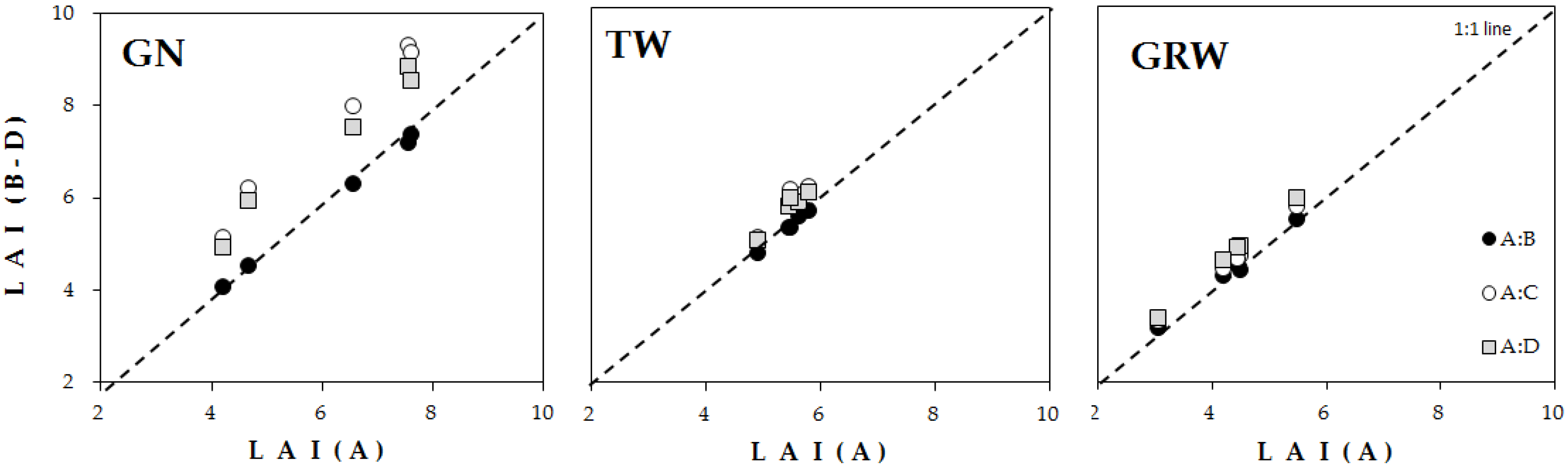
3.2. Estimation of LAI Based on Calculation Method

Four LAIs were estimated based on the calculation methods shown in Figure 1 by multiplying SLA from Table 3 with the average weight of leaves in five traps (Figure 2 and Figure A1). The maximum LAIs (mean ± SE) for each study site (i.e., the sums of all LAIs calculated for all periods), were in the order: B < A < D < C for GN; B < A < D < C for TH; and A = B < C < D for GRW (Table 4, Figure 3). Compared to method A (the reference method), method B showed a slight difference in GN (3%) and TH (2%), but the difference was not statistically significant in GRW (1%) (p > 0.05). The methods that showed the largest difference were method C in GN (25%) and TH (8%), and method D in GRW (9%). On the other hand, the largest spatial difference in the maximum LAI among five litter traps was in the ranges of 4.18–7.53 m2·m−2 in GN, 4.89–7.77 m2·m−2 in TH, and 3.06–5.47 m2·m−2 in GRW, with standard errors TH (0.05), GRW (0.33), and GN (1.04).
The maximum LAI calculated by method A showed that Q. serrata (2.97 m2·m−2) and C. laxiflora (1.85 m2·m−2), which are upper canopy species accounting for 90.3% of basal area in GN, accounted for 48.7% and 30.4% of the total LAIs, respectively. In TH, the LAI of the dominant species, Q. serrata, was 3.17 m2·m−2, accounting for 58.4% of the total, and LAIs of P. sargentii and Q. aliena were 0.68 m2·m−2 (12.5%) and 0.43 m2·m−2 (7.9%), respectively. In GRW, LAIs of upper canopy species were F. rhynchophylla 2.20 m2·m−2 (50.7%), S. alnifolia 0.44 m2·m−2 (10.1%), and K. septemlobus 0.10 m2·m−2 (2.4%), and the LAI of other lower canopy species was 1.59 m2·m−2 (36.7%). On the other hand, LAIs calculated for individual species using method B were: In GN, LAIs of Q. serrata (2.82 m2·m−2) and C. laxiflora (1.82 m2·m−2) were smaller than LAIs from method A by 5.2% and 1.8%, respectively; LAIs of C. cordata (0.24 m2·m−2), A. pseudosieboldianum (0.21 m2·m−2), and S. alnifolia (0.06 m2·m−2) were larger than LAIs from method A by 1.0%, 7.8%, and 2.0%, respectively. In TH, the LAI of Q. aliena from method B was larger than that from method A (0.433 m2·m−2) by 2.9%, but all other species showed smaller LAIs from method B than on method A. In contrast, in GRW, LAIs of all species were larger from method B than method A by up to 9.4%, such as F. rhynchophylla (2.268 m2·m−2), K. septemlobus (0.115 m2·m−2), S. alnifolia (0.454 m2·m−2), C. cordata (0.448 m2·m−2), and A. mono (0.310 m2·m−2).
Regarding LAIs from method A, the LAI in GN decreased by 5.02 m2·m−2, 82.3% of the total LAI, between day of year (DOY) 289 and DOY 308; and the LAI in TH decreased by 4.11 m2·m−2, 75.8% of the total LAI, between DOY 286 and DOY 315. However, in GRW, the LAI decreased rapidly by 3.06 m2·m−2 (70.5%) over a short period between DOY 272 and DOY 287, and showed an earlier start of the deciduous period compared to the other areas. Regarding LAI by period, calculated by method C, all three areas showed larger estimates compared to method A, with the exception of the LAI of DOY 324 in GRW (0.064 m2·m−2 from method A and 0.056 m2·m−2 from method C). Regarding the difference between estimates based on method A and method C on the day of the greatest number of fallen leaves in each plot of (GN, DOY 321; TH, DOY 315; and GRW, DOY 287), GN showed the highest difference (50.1%), followed by TH (9.0%) and GRW (5.5%).

4. Discussion

4.1. Temporal and Interspecific Variation of SLA

SLA, leaf area per unit mass, is one of speices specific characteristics but it shows spatial variation depending on vertical positions of trees within a stand and even depending on the location of a leaf within a canopy for the same tree [23,31]. This study also showed clear differences in SLA across different species due to individual species characteristics (Table 3), and SLA was smaller for upper than lower canopy species in all plots. This is caused by the strong negative correlation between SLA and the amount of light, and is consistent with the results of shading experiments for seedlings or understory trees showing high SLAs [32,33,34,35,36]. In particular, the present study showed that S. alnifolias, which grew in the lower canopy in GN and the upper canopy in GRW, showed 55.7% difference in SLA (GN 297.7 cm−2·g−1; and GRW 191.2 cm−2·g−1).
To determine SLA variation within the canopy, the coefficients of variation (CVs) for SLA of the upper and lower canopy species were compared. Upper canopy CVs are large within a canopy due to having a larger canopy compared to lower canopy species, in the range of 26%–46%, with mean = 34.8%, whereas the lower canopy species, which have shade-tolerant leaves that drop rapidly at the end of the deciduous period, had lower CVs with mean = 23.5%.
While SLA varied according to species and vertical positions, it showed no specific temporal patterns. In terms of temperate broadleaved forests in general, SLA gradually increased from September as leaves start withering due to suspension of physiological activities and retranslocation of nutrients from leaves to stems [37,38]. However, just as leaf unfolding can be either determinant or indeterminant depending on species, leaves can drop either from the center toward the outer crown (inner-type), or from the outer crown toward the center (outer-type) depending on tree species [39,40]. Accordingly, depending on species, shade leaves may drop first (inner type) or sun leaves drop first (outer type) [38,41]. In addition, differences in the degree of nutrient retranslocation and variations in meteorological factors, such as wind and precipitation, are likely to have physical effects on the canopy and contribute to large SLA variation across periods. SLA of the early September collection, which collected the leaves dropped throughout the month of August, was higher than the SLA of the mid-September collection. This reflects that the early-September collection included the leaves dropped for a whole month due to slower leaf falling process, compared to the mid-September collection, which only included leaves from a 15 day period. Hence, the former was in decomposition within the trap before retrieval due to leaching by frequent rain and high temperature and humidity in August [42].
Among the three stands with different ages and successional stages, the overall mean SLA was lowest in the youngest (TH). GN and GRW, which were more progressed in stand development, had more differentiated vertical canopy structures, which produced greater species and understory vegetation diversity, showing three major lower canopy species with high SLA in each stand. In contrast, the young matured stands (TH) showed lower mean SLA, because S. obassia was the only major lower canopy species in the stand due to a lack of vertical development resulting from competition among various canopy species (i.e., because a variety of canopy species with low SLA existed). Other species in GN and GRW were shade tolerant, including Symplocos chinensis, Styrax japonica, and Tilia amurensis, in contrast to TH, which had thick-leaved species, including Rhododendron mucronulatum and Rhododendron schlippenbachii. Consequently, SLA of other species was in the order: GN 262.1 cm2·g−1, GRW 186.7 cm2·g−1, and TH 175.2 cm2·g−1. This suggests that differences in stand composition as a result of their respective succession stages produced differences in overall SLA. In addition, the increased complexity of canopy structure with stand development could enhance the uncertainties of indirect methods due to the increased LAI and leaf clumping.

4.2. LAI Estimation Based on Four Calculation Methods

Considering SLA variation is important when estimating LAI using fallen leaves, because SLA varies across different time periods and tree species. Bouriaud et al. [9] studied the effects of SLA variation according to soil availability and collection dates in a pure Beech stand, and found that the SLA variation depending on plots caused an 8%–24% variation in LAI. Kalacska et al. [43] compared LAIs estimated by actual classification (method A in this study) and bootstrap estimation for various ways of averaging SLAs of 63 species, and found that LAIs were overestimated when different species were averaged, regardless of the number of species averaged. On that basis, they recommended considering SLAs of each species. Accordingly, LAI estimated using method A in the present study, which considered SLA of individual species and periods in calculation of LAI, is likely to be the most reliable method. However, consideration of interspecific and temporal variations could be limited, particularly in spatially and/or temporally large studies, due to time and labor consumption.
The LAI of method A was most similar to that of method B. Method B considered only interspecific SLA variation, and reduced LAI prediction error more than the other two methods, because SLAs showed no particular temporal variation pattern (Table 3). Conversely, when using Method C, which estimated overall period-specific SLA without considering the proportion of leaves by species, SLAs of species with lesser amounts of leaves (40 or less) were given the same weight in calculation as those of species with greater amounts of leaves. Hence, low height species with lesser amounts of leaves and higher SLAs had larger effects on the overall mean SLA than was representative, resulting in LAI overestimation. For example, on DOY 321 in GN, the difference in LAI between method A (2.48 m2·m−2) and C (3.72 m2·m−2) was maximum (50.1%). The overestimation from method C occurred because the amount of Q. serrata leaves on the day was high (70.6% of the total) so the mean SLA from method C was higher (255.7 cm2·g−1) than that of Q. serrata (147.3 cm2·g−1) used in method A.
The errors from methods C and D were greater in GN than in TH and GRW because GN has more varieties of lower canopy species with a smaller proportion of leaves but higher SLA due to vertical canopy development, as discussed above. Vertical canopy development also caused increase of LAI spatial variation (Figure 3). In contrast, GRW showed the lowest CVs of species specific importance, 36.7% (GN, 50.2%; TH, 65.9%) due to even species distribution, despite GRW having a larger LAI spatial variation than TH due to vertical canopy development. Consequently, the importance of species specific SLA decreased, and the error from method C and D was similar to TH, which showed low spatial LAI variation and small SLA due to a lack of lower canopy species varieties.
To avoid the effort of calculating SLA for each species in spatially and temporally large scale studies, we tried LAI estimation by obtaining only the SLA of upper canopy species and multiplying it by the total dry weight. In GN, the average SLA of Q. serrata and C. laxiflora was 197.33 cm2·g−1, generating LAI of 6.36 m2·m−2; in TH, the average SLA of Q. serrata, Q. aliena, and P. sargentii was 159.6 cm2·g−1, generating LAI of 5.417 m2·m−2; and in GRW, the average SLA of F. rhynchophylla, K. septemlobus, and S. alnifolia was 175.13 cm2·g−1, generating LAI of 4.11 m2·m−2. Differences between these LAIs and method A were (GN) 4.2%, (TH) 0.1%, and (GRW) 5.3%, which are similar to method B errors, suggesting that significant error reduction can be achieved by only considering SLAs of upper canopy species.

5. Conclusions

This study measured SLA of fallen leaves by tree species and collection dates in deciduous broadleaved forests of GN, TH, and GRW, and compared four LAI calculation methods. SLAs of individual species tended to be less for upper than lower canopy species, but neither upper nor lower canopy species showed specific temporal variation patterns. Among the four LAI calculation methods considered, method A (the reference method, which considers interspecific and temporal variation) and Method B (which used average SLA of each species) generated the most similar estimates, which clearly demonstrates the importance of interspecific variation in SLA. In particular, the importance was greater when the vertical development of canopy and presence of diverse lower-canopy vegetation increased as the stand ages. In contrast, in the stands of evenly distributed species (GRW) or less vertical differentiation (TH), the influence of interspecific SLA was lower. In other words, regarding LAI estimation, although Method A is most accurate, it is preferable to use the mean of each species as in Method B, or at least the mean SLA of dominant species over less accurate methods, unless the goal is to estimate the LAI reduction pattern. Therefore, it is likely to be feasible to estimate species-specific SLA by retrieval at two-week intervals or more frequently to prevent the decomposition of leaves prior to retrieving, drying, and storing them, and taking samples from the collected leaves.

Acknowledgments

This study was supported by the Korea Forest Service (Project No. S111212L20110 and S21134L020120) and 2014 Research Grant from Kangwon National University (No. C1010707-01-01). We thank the Korea National Arboretum in Gwangneung, Seoul National University Forest, and Korea National Forest Management Office for providing access to the study sites. Special thanks to all the participants for their help in the field survey and data processing. We acknowledge Prof. Kim for grammar assistance and anonymous reviewers for their valuable comments.

Author Contributions

All authors contributed substantially to the work reported here. The four authors participated in the conception and design of the study. Boram Kwon participated in the field data acquisition, analyzed the data, and wrote the manuscript. Hyun Seok Kim provided contributions in the collection, analyses, and interpretation of data and wrote the manuscript together with Boram Kwon. Jihyeon Jeon participated in the field data acquisition and in the laboratory investigation. Myong Jong Yi performed analysis of data and provided feedback and contributions to the written manuscript.

Conflicts of Interest

The authors declare no conflict of interest.

Appendix

Figure A1. Diagram of the SLA calculation methods for TH and GRW site (A: species- and collection date-specific SLA; B: species mean SLA with no consideration of seasonal variation; C: date-specific mean SLA neglecting species variation; and D: coarse, ignoring temporal and interspecific variation).
Forests 07 00215 g004

References

  1. Leverenz, J.W.; Hinckley, T.M. Shoot Structure, Leaf Area Index and Productivity of Evergreen Conifer Stands. Tree Physiol. 1990, 6, 135–149. [Google Scholar] [CrossRef] [PubMed]
  2. Chen, J.M. Optically-Based Methods for Measuring Seasonal Variation of Leaf Area Index in Boreal Conifer Stands. Agric. For. Meteorol. 1996, 80, 135–163. [Google Scholar] [CrossRef]
  3. Cutini, A.; Matteucci, G.; Mugnozza, G.S. Estimation of Leaf Area Index with the Li-Cor LAI 2000 in Deciduous Forests. For. Ecol. Manag. 1998, 105, 55–65. [Google Scholar] [CrossRef]
  4. Clark, D.B.; Olivas, P.C.; Oberbauer, S.F.; Clark, D.A.; Ryan, M.G. First Direct Landscape-scale Measurement of Tropical Rain Forest Leaf Area Index, a Key Driver of Global Primary Productivity. Ecol. Lett. 2008, 11, 163–172. [Google Scholar] [CrossRef] [PubMed]
  5. Eriksson, H.; Eklundh, L.; Hall, K.; Lindroth, A. Estimating LAI in Deciduous Forest Stands. Agric. For. Meteorol. 2005, 129, 27–37. [Google Scholar] [CrossRef]
  6. Osada, N.; Takeda, H.; Kawaguchi, H.; Furukawa, A.; Awang, M. Estimation of Crown Characters and Leaf Biomass from Leaf Litter in a Malaysian Canopy Species, Elateriospermum Tapos (Euphorbiaceae). For. Ecol. Manag. 2003, 177, 379–386. [Google Scholar] [CrossRef]
  7. Le Dantec, V.; Dufrêne, E.; Saugier, B. Interannual and Spatial Variation in Maximum Leaf Area Index of Temperate Deciduous Stands. For. Ecol. Manag. 2000, 134, 71–81. [Google Scholar] [CrossRef]
  8. Chen, J.; Black, T. Measuring Leaf Area Index of Plant Canopies with Branch Architecture. Agric. For. Meteorol. 1991, 57, 1–12. [Google Scholar] [CrossRef]
  9. Bouriaud, O.; Soudani, K.; Bréda, N. Leaf Area Index from Litter Collection: Impact of Specific Leaf Area Variability within a Beech Stand. Can. J. Remote Sens. 2003, 29, 371–380. [Google Scholar] [CrossRef]
  10. Chason, J.W.; Baldocchi, D.D.; Huston, M.A. A Comparison of Direct and Indirect Methods for Estimating Forest Canopy Leaf Area. Agric. For. Meteorol. 1991, 57, 107–128. [Google Scholar] [CrossRef]
  11. Breda, N.J. Ground-Based Measurements of Leaf Area Index: A Review of Methods, Instruments and Current Controversies. J. Exp. Bot. 2003, 54, 2403–2417. [Google Scholar] [CrossRef] [PubMed]
  12. Jonckheere, I.; Fleck, S.; Nackaerts, K.; Muys, B.; Coppin, P.; Weiss, M.; Baret, F. Review of Methods for in Situ Leaf Area Index Determination: Part I. Theories, Sensors and Hemispherical Photography. Agric. For. Meteorol. 2004, 121, 19–35. [Google Scholar] [CrossRef]
  13. Gower, S.T.; Kucharik, C.J.; Norman, J.M. Direct and Indirect Estimation of Leaf Area Index, F APAR, and Net Primary Production of Terrestrial Ecosystems. Remote Sens. Environ. 1999, 70, 29–51. [Google Scholar] [CrossRef]
  14. Weiss, M.; Baret, F.; Smith, G.; Jonckheere, I.; Coppin, P. Review of Methods for in Situ Leaf Area Index (LAI) Determination: Part II. Estimation of LAI, Errors and Sampling. Agric. For. Meteorol. 2004, 121, 37–53. [Google Scholar] [CrossRef]
  15. Watanabe, T.; Yokozawa, M.; Emori, S.; Takata, K.; Sumida, A.; Hara, T. Developing a Multilayered Integrated Numerical Model of Surface Physics-Growing Plants Interaction (MINoSGI). Glob. Chang. Biol. 2004, 10, 963–982. [Google Scholar] [CrossRef]
  16. Walcroft, A.; Brown, K.; Schuster, W.; Tissue, D.; Turnbull, M.; Griffin, K.; Whitehead, D. Radiative Transfer and Carbon Assimilation in Relation to Canopy Architecture, Foliage Area Distribution and Clumping in a Mature Temperate Rainforest Canopy in New Zealand. Agric. For. Meteorol. 2005, 135, 326–339. [Google Scholar] [CrossRef]
  17. Wang, X.; Wang, X.; Yan, E. Leaf Nutrient Concentration, Nutrient Resorption and Litter Decomposition in an Evergreen Broad-Leaved Forest in Eastern China. For. Ecol. Manag. 2007, 239, 150–158. [Google Scholar]
  18. Bondeau, A.; Kicklighter, D.W.; Kaduk, J.; Intercomparison, T. Participants of the Potsdam NpP. Model Intercomparison. Comparing Global Models of Terrestrial Net Primary Productivity (NPP): Importance of Vegetation Structure on Seasonal NPP Estimates. Glob. Chang. Biol. 1999, 5, 35–45. [Google Scholar] [CrossRef]
  19. Song, Y.; Ryu, Y. Seasonal Changes in Vertical Canopy Structure in a Temperate Broadleaved Forest in Korea. Ecol. Res. 2015, 30, 821–831. [Google Scholar] [CrossRef]
  20. Dufrêne, E.; Bréda, N. Estimation of Deciduous Forest Leaf Area Index using Direct and Indirect Methods. Oecologia 1995, 104, 156–162. [Google Scholar] [CrossRef]
  21. McCarthy, H.R.; Oren, R.; Finzi, A.C.; Ellsworth, D.S.; Kim, H.; Johnsen, K.H.; Millar, B. Temporal Dynamics and Spatial Variability in the Enhancement of Canopy Leaf Area Under Elevated Atmospheric CO2. Glob. Chang. Biol. 2007, 13, 2479–2497. [Google Scholar] [CrossRef]
  22. Garcia, R.L.; Norman, J.M.; McDermitt, D.K. Measurements of Canopy Gas Exchange using an Open Chamber System. Remote Sens. Rev. 1990, 5, 141–162. [Google Scholar] [CrossRef]
  23. Ellsworth, D.; Reich, P. Canopy Structure and Vertical Patterns of Photosynthesis and Related Leaf Traits in a Deciduous Forest. Oecologia 1993, 96, 169–178. [Google Scholar] [CrossRef]
  24. Poorter, H.; Niinemets, Ü.; Poorter, L.; Wright, I.J.; Villar, R. Causes and Consequences of Variation in Leaf Mass per Area (LMA): A Meta-analysis. New Phytol. 2009, 182, 565–588. [Google Scholar] [CrossRef] [PubMed]
  25. Liu, Z.; Jin, G.; Chen, J.M.; Qi, Y. Evaluating Optical Measurements of Leaf Area Index Against Litter Collection in a Mixed Broadleaved-Korean Pine Forest in China. Trees 2015, 29, 59–73. [Google Scholar] [CrossRef]
  26. Clough, B.; Tan, D.T.; Buu, D.C. Canopy Leaf Area Index and Litter Fall in Stands of the Mangrove Rhizophora Apiculata of Different Age in the Mekong Delta, Vietnam. Aquat. Bot. 2000, 66, 311–320. [Google Scholar] [CrossRef]
  27. Braun, E.L. Deciduous Forests of Eastern North America; Blakiston Co.; Blakiston Co.: Philadelphia, PA, USA, 1950. [Google Scholar]
  28. Kim, H.; Lee, M.; Kim, S.; Guenther, A.B.; Park, J.P.; Cho, G.; Kim, H. Measurements of Isoprene and Monoterpenes at Mt. Taewha and Estimation of their Emissions. Korean J. Agric. For. Meteorol. 2015, 17, 217–226. [Google Scholar] [CrossRef]
  29. Ryu, Y.; Lee, G.; Jeon, S.; Song, Y.; Kim, H. Monitoring Multi-Layer Canopy Spring Phenology of Temperate Deciduous and Evergreen Forests using Low-Cost Spectral Sensors. Remote Sens. Environ. 2014, 149, 227–238. [Google Scholar] [CrossRef]
  30. Kang, M.; Kwon, H.; Lim, J.; Kim, J. Understory Evapotranspiration Measured by Eddy-Covariance in Gwangneung Deciduous and Coniferous Forests. Korean J. Agric. For. Meteorol. 2009, 11, 233–246. [Google Scholar] [CrossRef]
  31. Lichtenthaler, H.K.; Babani, F.; Langsdorf, G. Chlorophyll Fluorescence Imaging of Photosynthetic Activity in Sun and Shade Leaves of Trees. Photosynth. Res. 2007, 93, 235–244. [Google Scholar] [CrossRef] [PubMed]
  32. Anten, N.P.; Hirose, T. Interspecific Differences in Above-ground Growth Patterns Result in Spatial and Temporal Partitioning of Light among Species in a Tall-grass Meadow. J. Ecol. 1999, 87, 583–597. [Google Scholar] [CrossRef]
  33. Niinemets, U. Photosynthesis and Resource Distribution through Plant Canopies. Plant Cell Environ. 2007, 30, 1052–1071. [Google Scholar] [CrossRef] [PubMed]
  34. Van Hees, A.; Clerkx, A. Shading and Root–Shoot Relations in Saplings of Silver Birch, Pedunculate Oak and Beech. For. Ecol. Manag. 2003, 176, 439–448. [Google Scholar] [CrossRef]
  35. Dewar, R.C.; Tarvainen, L.; Parker, K.; Wallin, G.; McMurtrie, R.E. Why does Leaf Nitrogen Decline within Tree Canopies Less Rapidly than Light? An Explanation from Optimization Subject to a Lower Bound on Leaf Mass Per Area. Tree Physiol. 2012, 32, 520–534. [Google Scholar] [CrossRef] [PubMed]
  36. Peltoniemi, M.S.; Duursma, R.A.; Medlyn, B.E. Co-Optimal Distribution of Leaf Nitrogen and Hydraulic Conductance in Plant Canopies. Tree Physiol. 2012, 32, 510–519. [Google Scholar] [CrossRef] [PubMed]
  37. Santa Regina, I.; Leonardi, S.; Rapp, M. Foliar Nutrient Dynamics and Nutrient-use Efficiency in Castanea Sativa Coppice Stands of Southern Europe. Forestry 2001, 74, 1–10. [Google Scholar] [CrossRef]
  38. Koike, T. Autumn Coloring, Photosynthetic Performance and Leaf Development of Deciduous Broad-Leaved Trees in Relation to Forest Succession. Tree Physiol. 1990, 7, 21–32. [Google Scholar] [CrossRef] [PubMed]
  39. Kikuzawa, K. Leaf Survival of Woody Plants in Deciduous Broad-Leaved Forests. I. Tall Trees. Can. J. Bot. 1983, 61, 2133–2139. [Google Scholar]
  40. Koike, T. Leaf Structure and Photosynthetic Performance as Related to the Forest Succession of Deciduous Broad-Leaved Trees. Plant Species Biol. 1988, 3, 77–87. [Google Scholar] [CrossRef]
  41. Kitaoka, S.; Koike, T. Seasonal and Yearly Variations in Light use and Nitrogen use by Seedlings of Four Deciduous Broad-Leaved Tree Species Invading Larch Plantations. Tree Physiol. 2005, 25, 467–475. [Google Scholar] [CrossRef] [PubMed]
  42. Couteaux, M.; Bottner, P.; Berg, B. Litter Decomposition, Climate and Liter Quality. Trends Ecol. Evol. 1995, 10, 63–66. [Google Scholar] [CrossRef]
  43. Kalacska, M.; Calvo-Alvarado, J.C.; Sanchez-Azofeifa, G.A. Calibration and Assessment of Seasonal Changes in Leaf Area Index of a Tropical Dry Forest in Different Stages of Succession. Tree Physiol. 2005, 25, 733–744. [Google Scholar] [CrossRef] [PubMed]
Figure 1. Diagram of the specific leaf area (SLA) calculation methods (A: species- and collection date-specific SLA; B: species mean SLA with no consideration of seasonal variation; C: date-specific mean SLA neglecting species variation; and D: coarse, ignoring temporal and interspecific variation).
Forests 07 00215 g001
Figure 2. Diagram of the SLA calculation methods for GN (A: species- and collection date-specific SLA; B: species mean SLA with no consideration of seasonal variation; C: date-specific mean SLA neglecting species variation; and D: coarse, ignoring temporal and interspecific variation).
Forests 07 00215 g002
Figure 3. Diagram of the SLA calculation methods (A: species- and collection date-specific SLA; B: species mean SLA with no consideration of seasonal variation; C: date-specific mean SLA neglecting species variation; and D: coarse, ignoring temporal and interspecific variation).
Forests 07 00215 g003
Table 1. Selected characteristcs of three study sites in deciduous broadleaved forests, Korea.
Site *GN *TH †GRW ‡
Elevation (m)2562421199
Slope steepness (%)18833
Aspect (°)11010355
Species (density (number of stems ha−1), relative basal area (%))Quercus mongolica (128, 75.0), Carpinus laxiflora (96, 15.5), Others (752, 9.5)Q. mongolica (550, 72.2), Q. aliena (75, 10.9), Others (625, 17.0)Fraxinus rhynchophylla (224, 44.2), Kalopanax septemlobus (48, 22.9), Sorbus alnifolia (48, 13.7) Others (672, 19.2)
* GN, Gwangneung Arboretum; † TH, Mt. Taehwa; ‡ GRW, Mt. Gariwangsan.
Table 2. Two-way Analysis of Variance on SLA between species and collection dates from the three study sites.
SiteSourceType III Sum of SquaresDfMean SquareFp-Value
GN *Corrected Model4,208,254.826 *34123,772.20130.2370.000
Intercept13,156,498.857113,156,498.8573214.1270.000
Species1,654,488.7625330,897.75280.8380.000
Collection Dates240,640.423640,106.7379.7980.000
Species × Collection Dates556,636.6152324,201.5925.9120.000
Error3,610,321.2808824093.335
Total53,337,330.131917
Corrected Total7,818,576.106916
TH Corrected Model992,829.674 3033,094.3226.9760.000
Intercept4,842,026.86614,842,026.8661020.6050.000
Species222,195.659455,548.91511.7090.000
Collection Dates132,159.957622,026.6594.6430.000
Species × Collection Dates164,700.465208235.0231.7360.024
Error3,420,620.3537214744.272
Total25,972,407.402752
Corrected Total4,413,450.026751
GRW Corrected Model2,267,049.395 3761,271.60515.2490.000
Intercept7,261,444.89517,261,444.8951807.2240.000
Species780,273.6206130,045.60332.3660.000
Collection Dates117,973.814523,594.7635.8720.000
Species × Collection Dates476,833.7822618,339.7614.5640.000
Error3,439,416.9998564018.011
Total42,054,738.045894
Corrected Total5,706,466.394893
* R Squares = 0.538 (Collected R Squares = 0.520); R Squares = 0.225 (Collected R Squares = 0.193); R Squares = 0.397 (Collected R Squares = 0.371).
Table 3. Seasonal variation of SLA for individual species from the three study sites.
SiteSpeciesSLA (cm2·g−1)
SeptemberSeptemberOctoberOctoberNovemberNovemberDecemberAvg.
-Early-Mid-Early-Mid-Early-Mid-Early
GNQuercus serrata136.3 ± 4.3Aabc125.4 ± 7.3Aa132.3 ± 9.8Aab126.9 ± 3.8Aa152.0 ± 4.6Ac147.3 ± 5.6Abc154.6 ± 7.0Ac139.3 ± 2.1A
(n = 72)(n = 23)(n = 17)(n = 55)(n = 49)(n = 51)(n = 21)(n = 288)
Carpinus laxflora301.1 ± 14.5Bc177.7 ± 6.8Aa283.3 ± 14.0Bbc232.1 ± 11.1BCb261.6 ± 7.4Bbc290.5 ± 8.7CDbc247.6 ± 23.6Bbc249.9 ± 4.8B
(n = 38)(n = 70)(n = 50)(n = 58)(n = 54)(n = 45)(n = 3)(n = 318)
Carpinus cordata340.8 ± 18.8Bd173.1 ± 72.3Aa283.5 ± 47.4Bbcd223.6 ± 12.9Bab256.6 ± 10.7Bbc314.4 ± 11.6Dcd345.5 ± 10.1Cd286.2 ± 8.4D
(n = 10)(n = 2)(n = 4)(n = 14)(n = 13)(n = 19)(n = 7)(n = 69)
Acer pesudosieboldianum--245.6 ± 11.2Ba311.7 ± 35.7Da251.7 ± 17.0Ba290.7 ± 13.3CDa293.4 ± 36.9BCa279.9 ± 9.7CD
(n = 2)(n = 5)(n = 12)(n = 18)(n = 4)(n = 41)
Sorbus alnifola----319.6 ± 8.6C*273.8 ± 21.7C *-297.7 ± 12.1D
(n = 12)(n = 11)(n = 23)
Others 325.2 ± 41.1Bd113.4 ± 28.1Aa314.1 ± 36.2Bcd279.9 ± 11.4CDcd278.9 ± 10.3Bcd218.0 ± 13.2Bbc169.1 ± 27.1Aab262.1 ± 6.9BC
(n = 3)(n = 7)(n = 7)(n = 56)(n = 70)(n = 32)(n = 3)(n = 178)
Total208.5 ± 9.5b161.4 ± 5.9a253.0 ± 12.0c217.0 ± 6.8b244.2 ± 5.6c237.4 ± 6.5c212.9 ± 14.1b222.8 ± 3.1
(n = 123)(n = 102)(n = 80)(n = 188)(n = 210)(n = 176)(n = 38)(n = 917)
THQuercus serrata150.9 ± 5.5Aa121.4 ± 10.3Aa145.8 ± 10.7Aa130.8 ± 6.5Aa151.1 ± 6.9Aa154.3 ± 19.3Aa155.7 ± 6.0Aa146.6 ± 4.3A
(n = 22)(n = 13)(n = 12)(n = 45)(n = 39)(n = 41)(n = 52)(n = 224)
Quercus aliena148.7 ± 14.1Aab110.4 ± 8.6Aa125.3 ± 10.9Aa161.4 ± 28.8ABab140.8 ± 9.0Aab121.9 ± 7.1Aa196.8 ± 17.1Ab138.8 ± 6.6A
(n = 8)(n = 16)(n = 2)(n = 16)(n = 9)(n = 33)(n = 10)(n = 94)
Prunus sargentii179.8 ± 12.2Aa198.4 ± 11.2Ba166.3 ± 6.3Aa185.0 ± 9.0Ba197.1 ± 9.8Ba190.5 ± 26.6Aa318.6 **182.0 ± 4.1B
(n = 27)(n = 22)(n = 78)(n = 43)(n = 41)(n = 5)(n = 1)(n = 217)
Styrax obassia--162.0 ± 37.5Aa-291.8 ± 11.1Cb288.7 ± 15.5Bb-284.0 ± 10.2C
(n = 2)(n = 27)(n = 7)(n = 36)
Others ††156.4 ± 17.6Aa62.4 **107.7 ± 4.7Aa170.3 ± 13.7Ba173.3 ± 11.4ABa189.6 ± 12.9Aa309.0 ± 33.3Bb175.2 ± 6.7B
(n = 10)(n = 1)(n = 7)(n = 39)(n = 65)(n = 57)(n = 2)(n = 181)
Total163.1 ± 6.2a149.4 ± 8.4a158.9 ± 5.3a161.3 ± 6.2a190.0 ± 6.2b168.7 ± 8.4bc169.2 ± 7.0bc169.3 ± 2.8
(n = 67)(n = 52)(n = 101)(n = 143)(n = 181)(n = 143)(n = 65)(n = 752)
GRWFraxinus rhynchophylla152.6 ± 12.5Aab183.1 ± 14.3Aab192.6 ± 8.0Ab166.6 ± 4.0Bab118.1 ± 6.1Aa186.0 ± 49.1ABb-171.9 ± 3.4B
(n = 24)(n = 13)(n = 59)(n = 157)(n = 2)(n = 3)(n = 258)
Kalopanax septemlobus196.1 ± 31.4ABa188.4 ± 15.1Abc-120.8 ± 9.5Aa143.9 ± 10.9Aab -146.9 ± 8.9A
(n = 3)(n = 5)(n = 13)(n = 5)(n = 26)
Sorbus alnifola200.4 ± 16.7ABa162.3 ± 14.4Aa223.6 ± 18.8Aab176.3 ± 8.6Ba222.0 ± 12.1Bab273.5 ± 46.4Bb-191.2 ± 6.4BC
(n = 12)(n = 15)(n = 15)(n = 44)(n = 8)(n = 3)(n = 97)
Carpinus cordata324.3 ± 22.7Cb281.9 ± 15.9Bab255.1 ± 20.2Aa270.6 ± 9.3Da321.1 ± 10.3Ca--294.1 ± 6.5E
(n = 20)(n = 21)(n = 9)(n = 46)(n = 40)(n = 136)
Acer pesudosieboldianum-258.1 ± 43.6Ba252.9 ± 60.0Aa225.7 ± 5.8Ca287.3 ± 17.6BCa247.1 **-237.2 ± 6.5D
(n = 2)(n = 2)(n = 29)(n = 5)(n = 1)(n = 39)
Acer mono238.2 ± 16.5ABCa192.8 ± 18.5Aa203.4 ± 12.3Aa193.3 ± 8.5Ba240.5 ± 16.6Ba134.9 **-202.3 ± 6.1C
(n = 8)(n = 7)(n = 11)(n = 44)(n = 6)(n = 1)(n = 77)
Others 285.1 ± 30.5BCd190.1 ± 8.6Ac212.8 ± 11.3Ac174.8 ± 6.2Bbc129.2 ± 7.5Aab107.7 ± 15.4Aa-186.7 ± 5.2BC
(n = 21)(n = 30)(n = 60)(n = 109)(n = 37)(n = 4)(n = 261)
Total239.0 ± 12.1c207.0 ± 7.2ab208.5 ± 5.9ab185.6 ± 3.1a225.6 ± 10.0bc182.6 ± 25.2a-201.6 ± 2.7
(n = 88)(n = 93)(n = 156)(n = 442)(n = 103)(n = 12)(n = 894)
Means ± Standard error were followed by alphabet letters to represent statistically significant differences at p = 0.05 level according to the Duncan test for each study site (upper-case alphabet letters indicate differences among species in the same collect date, lower-case alphabet letters demonstrate differences among collect dates for each species). The numbers in parentheses represent sampling numbers of measured SLA. * indicates no differences between two dates. ** indicates exclusion from statistical analysis due to small sample size. Styrax japonica, Euonymus sachalinensis, Symplocos chinensis, Styrax obassia; †† Rhododendron mucronulatum, Rhododendron yedoense, Symplocos chinensis; Acer mandshuricum, Tilia amurensis.
Table 4. Comparison of leaf area index estimates from four different methods.
ABCDA vs. BA vs. CA vs. D
GN6.09 ± 0.725.91 ± 0.687.59 ± 0.827.18 ± 0.750.030.250.18
TH5.42 ± 0.155.34 ± 0.155.87 ± 0.205.75 ± 0.180.020.080.06
GRW4.33 ± 0.394.37 ± 0.374.57 ± 0.394.73 ± 0.410.010.060.09

