1. Introduction
Leaf area index (LAI) is an important variable for understanding architecture and biological processes in trees [
1], designing silvicultural treatments [
2], for landscape-level ecosystem process models [
3], or global forest functions [
4]. LAI has been defined as the sum of projected (one-sided), or all-sided leaf areas, for all trees in a given area divided by the land surface area the trees cover [
5]. Hence, in equal units, LAI becomes a unitless measure of leaf surface area per unit of land surface area covered.
LAI has great utility as a tool for both science and management; however, it is difficult to quantify because of the structural complexity and temporal variation of leaf display in forests [
6]. Additionally, there is enormous variation in leaf morphology and physiology among vascular plant species [
7,
8]. A unit of leaf area in one species may therefore not equate to similar levels of, for example, light interception, photosynthesis, or water usage in a different species. Hence, procedures that integrate species composition into LAI estimates will provide better estimates of physiological functions at all scales of forest cover.
Several methods of LAI estimation have been developed [
9,
10,
11,
12,
13]. Direct methods include destructive sampling to measure actual leaf area or collection and measurement of leaf litter. Leaf litter can be sorted and leaf area determined for each species. Indirect methods include optical techniques that measure light extinction through the canopy, or hemispherical photography that estimates LAI based on geometry of canopy openings. Measures of light extinction or hemispherical photography do not differentiate LAI by species, but instead can estimate total LAI inclusive of all species. Another indirect method relies on the allometric relationship between tree leaf area and tree dimensions to estimate tree leaf area, which is summed by tree and divided by land surface area to get LAI. LAI can also be estimated through remote sensing, such as with aerial or ground-based LIDAR, which has the potential to estimate leaf area by tree or species [
14,
15].
Of these methods, estimating LAI using individual tree allometries is the only method, at present, that can be used to easily estimate LAI by individual trees, species, age classes, or canopy strata. Understanding the distribution of LAI by these stand components provides advantages for describing stand structure, and modeling changes in structure through silvicultural interventions [
16].
Allometries in plants are generally assumed to follow fundamental metabolic scaling rules related to annual growth rates [
17]. For trees, the pipe model theory, generally credited to Shinozaki and others [
18,
19,
20,
21,
22,
23,
24], forms the theoretical basis for allometric proportionalities between tree leaf area, or foliage mass, above a point in the crown and the cross-sectional area of conducting tissues at that point on the stem. In small trees, where all xylem may be functional conducting tissue, the pipe model indicates a relationship between tree cross-sectional area, or basal area, and leaf area. However, in larger trees with non-conducting xylem, or heartwood, the relationship is theoretically strongest when sapwood cross-sectional area at the base of live crown is used to predict leaf area due to sapwood taper [
24,
25,
26]. Hence, leaf area prediction models have often been based on sapwood cross-sectional area at the base of the live crown or with a variable to represent crown height [
24,
25,
27].
Development of leaf area prediction relationships requires laborious foliage sampling to estimate leaf surface area. Whereas most previous studies used a single procedure, fewer studies have compared alternative procedures [
9,
11,
12,
13,
28,
29,
30,
31]. Our analysis used a variety of conifer species from the mixed-conifer forests of the Sierra Nevada in California, including shade intolerant and tolerant species, to compare procedures for tree leaf area prediction, and to develop a partially destructive sampling approach.
Leaf area relationships are typically developed by scaling leaf area from branch to tree using either a crown section [
31,
32], or a branch summation approach [
33,
34], on cut trees. The crown section approach estimates leaf area by crown section, usually crown thirds, whereas the branch summation estimates leaf area from individual tree branch allometries developed from a subsample of branches. We compared results from these two procedures and a partially-destructive extension of the branch summation approach where trees were climbed and cored instead of cut down.
Several previous studies have explored alternative methods to predict tree leaf area from DBH, or other external tree features that require no destructive sampling or coring [
32,
33,
35]. We tested several model forms to predict one-sided leaf area of branches, crown portions and whole trees using several external tree features as covariates. We also tested model forms that predict one-sided whole tree leaf area from measured sapwood cross-sectional area at 1.37 m height. We used nonlinear mixed effects (NLME) modeling techniques described in Pinheiro and Bates [
36] to account for random effects for site and tree as well as to assess impacts of additional covariates on model parameter estimates.
The goal of this study was to compare alternative sampling procedures and models for estimating one-sided tree leaf area in temperate conifers using the advantages of mixed effects modeling to compare alternate model forms. Specifically, our objectives were to:
Develop leaf area prediction models for tree branches for several coniferous species across a wide range of environmental conditions;
Develop leaf area prediction models for a portion of the live crown;
Compare the performance of several whole tree leaf area prediction model forms and primary covariates;
Determine the impact of sampling procedures on whole tree leaf area prediction models; and
Determine the impact of additional covariates on the leaf area prediction models developed in objectives 1–3 using NLME techniques.
2. Experimental Section
2.1. Sample Sites
Trees were sampled from six locations in the Sierra Nevada (
Table 1), using two different primary sampling procedures. The two primary sampling procedures were the crown section approach (D1) described in [
31,
37,
38], and the branch summation approach (D2) described in [
33]. Sampled stands ranged from even-aged, to multiaged, stand structures and were typically on productive sites in the mixed-conifer forests of the Sierra Nevada. Species sampled were: sugar pine (
Pinus lambertiana Dougl.), ponderosa pine (
P. ponderosa Lawson & C. Lawson), Jeffrey pine (
P. jeffreyi Balf.), coast Douglas-fir (
Pseudotsuga menziesii (Mirb.) Franco var.
menziesii), white fir (
Abies concolor (Gord. & Glend.) Lindl. ex Hildebr.), red fir (
A. magnifica A. Murray), and incense-cedar (
Calocedrus decurrens (Torr.) Florin). Jeffrey pine was the only species sampled at the Bureau of Land Management site, and red fir was the only species sampled at the Teakettle Experimental Forest. Douglas-fir was not present in the Southern California Edison site. All other species occurred at every site and were sampled across a wide range of diameters at each location. Summary data for sampled trees can be found in
Table 2.
Table 1.
Summary information for study sites for each sampling category.
Table 1.
Summary information for study sites for each sampling category.
| Ownership/Location Name | Latitude | Longitude | Elevation Range (m) | Sampling Category | Age Structure |
|---|
| Baker Forest | 39.91° | −121.06° | 1211–1347 | D2 | Even-aged & multiaged |
| Bureau of Land Management | 39.67° | −120.16° | 1764–1768 | D2 | Multiaged |
| Blodgett Forest Research Station | 38.91° | −120.66° | 1250–1338 | D1 & D2 | Even-aged & multiaged |
| Southern California Edison | 37.04° | −119.21° | 1584–1594 | D2 | Multiaged |
| Sierra Pacific Industries | 38.75° | −120.75° | 1309–1650 | D1 | Even-aged |
| Teakettle Experimental Forest | 36.96° | −119.02° | 2062–2074 | D2 | Multiaged |
Table 2.
Summary tree statistics.
Table 2.
Summary tree statistics.
| Species | Mean DBH (cm) | Mean HT (m) | Mean HLC (m) | n D1 | n D2 |
|---|
| Douglas-fir | 28.5 (19.5) | 18.3 (11.2) | 5.9 (5.5) | 7 | 7 |
| Incense-cedar | 34.4 (25.6) | 16.3 (9.6) | 5.6 (3.4) | 7 | 14 |
| Jeffrey pine | 20.4 (12.6) | 8.9 (4.7) | 1.4 (0.8) | 0 | 5 |
| Ponderosa pine | 29.2 (21.6) | 17.4 (11.6) | 6.6 (5.4) | 9 | 12 |
| Red fir | 19.4 (12.4) | 12.5 (7.8) | 1.9 (0.9) | 0 | 5 |
| Sugar pine | 37.5 (29.8) | 19.5 (11.7) | 6.7 (6.0) | 7 | 11 |
| White fir | 30.0 (25.2) | 16.9 (10.8) | 4.8 (4.3) | 7 | 14 |
2.2. Sapwood Area Sampling Procedure
Cross-sectional sapwood area was determined by destructive and nondestructive sampling. Destructive sampling consisted of cutting tree discs from stump height, 1.37 m (breast height), live crown base, and every 2 m within the live crown. Tree discs were photographed in the field with a metric ruler placed on their surface for scale. Digital calibration was used to measure total disc area, sapwood area, heartwood area, and bark area. The accuracy of digital calibration was checked along multiple points of the ruler and deviation was kept below 0.5% for all disc measurements. Nondestructive sampling utilized cores taken at 1.37 m, base of live crown, and every 4 m within the tree crown until climbing was no longer safe. Cores were taken outside bark crevices so as to include maximum bark thickness. Total inside bark area was determined by subtracting double bark thickness from the measured diameter at core extraction point. Heartwood radius was calculated by determining the inside bark radius minus sapwood thickness and then used to calculate heartwood area. Sapwood cross-sectional area was determined by subtracting heartwood area from total inside bark area. A linear regression of sapwood area against basal area was performed to determine the nature of the relationship between those two covariates.
2.3. Leaf Area Sampling Procedures
Three alternative leaf area sampling procedures were used: crown section, branch summation, and a partially-destructive extension of the branch summation approach. The crown section approach divides the crown into sections (usually thirds) that are sampled as separate units [
31,
32]. We weighed the live branches and foliage from each section in the field. A representative branch, and associated foliage, from each crown third was removed from the stem for analysis in the lab. Subsamples of foliage from selected branches were scanned for one-sided leaf area and oven-dried in the lab to determine dry weight to field weight ratios, and specific leaf area (leaf area/foliar mass). Remaining branch material, and the rest of the branch foliage, were also oven-dried, and field weight to dry weight ratios calculated. The field weight of each section was converted to dry branch and foliage weight using ratios calculated in the lab, and the measured specific leaf area was used to estimate leaf area of the crown section based on foliar masses. Whole tree leaf area was calculated as the sum of crown section leaf areas.
The branch summation approach develops a relationship between branch diameter and leaf area that is applied to each branch within a tree or section of tree crown [
24,
38]. The diameter of all branches was measured outside the branch collar on both the major and minor axes. Random branches were removed for lab analysis of wet and dry foliage weights and leaf area. Branch leaf area prediction equations were developed and applied to all measured branches using the models for branch leaf area found in
Table 3. Branch leaf areas were summed for whole tree leaf area for destructively sampled trees.
Table 3.
Summary of candidate leaf area prediction models sorted by associated tree feature. References given for existing leaf area models taken from the literature.
Table 3.
Summary of candidate leaf area prediction models sorted by associated tree feature. References given for existing leaf area models taken from the literature.
| Tree Feature | Model | Model Form | Reference |
|---|
| Tree Branch | 1 | b1BRAe−(RDC/b2)b3 | |
| 2 | b1BRAb2(b3/b4)(RDC/b4)(b3 − 1)e−(RDC/b4) b3 | |
| 3 | b1BRA(RDC/b3)(b2 − 1)e−(RDC/b3)b2 | |
| 4 * | b1BRAb2RDC(b3 − 1)e−RDCb3 + ϕi | |
| 5 | (b1BRA(1/3) + b2RDC(1/3))3 | [33] |
| 6 | b1BRAb2(HT − BHT) | [39] |
| Whole Tree | 7 | b1X/(b2 + X) | [40] |
| 8 | b1Xb2 | |
| 9 | b1/(1 − e((b2−X)/b3)) | |
| 10 | b1X | |
| 11 | b1X + b2 | |
| 12 * | b1X•BHCRb2 + ϕi | [41] |
| 13 * | b1Xb2BHCRb3 + ϕi | |
| 14 | b1X + b2(HLC − 1.37) | [42] |
| 15 | eb1•ln(X) | [43] |
| 16 | b1 + b2X + b3CL | [44] |
| 17 | e(b1•ln(X)+b2•ln(CL)) | [35] |
| 18 | e(b1Xb2CLb3) | [35] |
| 19 * | b1(X(1 − e−X))b2 + ϕi | |
| 20 | b1(X(1 − e−X/b2))b3 | |
| 21 | b1X(1 − e(−X/b2)b3)) | |
| 22 | b1Xb2(1 − e−X/b3) | |
| 23 | b1Xb2(1 − e−Xb3) | |
| 24 | b1X(1 − e−X/b2) | |
| 25 | b1X(1 − e−Xb3)) | |
| 26 | b1X(1 − e−X) | |
| Crown Portion | 27 | b1SWPVb2(1 − e−b3eb4RDC) | |
| 28 | b1SWPVb2/(1 + e(b3−RDC)/b4) | |
| 29 | b1SWPV/(b2 + SWPV) | |
| 30 * | b1(SWPV(1 − e−RDCb2))b3 + ϕi | |
| 31 * | b1(SWPV(1 − e−(RDC/b4)b2))b3 + ϕi | |
| 32 | b1RDCb2SWPVb3 | |
| 33 | b1SWPVb2(b3/b4)(RDC/b4)(b3−1) e(−RDC/b4)b3 | |
| 34 | b1SWPVb2 + b3 | |
Our new, partially destructive, sampling procedure extends the branch summation approach to larger trees that may be difficult to destructively sample. This new approach utilized the same methods as branch summation with two critical differences; sapwood was measured with cores not discs, and upper portions of the crown that could not be measured were estimated using species specific crown portion leaf area models. The crown portion leaf area model development is described below.
Foliage subsamples from all procedures were scanned using a digital scanner and analyzed for one-sided leaf area using Regent Instruments WinFolia software package (Reg 2001a, Regent Instruments, Quebec, QC, Canada). The subsample foliage was then placed in small paper bags and oven dried to a constant mass, along with the remaining foliage.
2.4. Leaf Area Data Categorization and Crown Portion Leaf Area Sampling Procedures
Trees destructively sampled using the crown section approach were assigned a category label D1. Trees sampled using the branch summation approach were assigned a category label D2. Trees in the D2 category were subcategorized as destructive (D2D, sapwood measures from discs), or partially-destructive (D2C, sapwood measures from cores) samples. The D2C category contains all of the data for the new method developed in this study. Partially-destructive sampling required climbing trees and taking cores along the tree bole. The decision of whether a tree could be climbed was made on a tree-by-tree basis and primarily driven by concerns for climber safety. The cores extracted along the bole were used to estimate sapwood area instead of using discs, as was done for trees in the D2D category. Branch diameter measurements were collected while climbing up the tree up until it was no longer safe to climb. Because trees could not be climbed all the way to the top, a separate model was developed to predict the leaf area of the missing crown portion based on data from sampled trees in the D2D category. Therefore, whole tree leaf area data consisted of leaf area estimates from three different sampling procedures, D1, D2D, and D2C.
2.5. Leaf Area Prediction Modeling
Leaf area prediction models were developed for three tree features, branch, crown portion, and whole tree. A list of candidate leaf area models for each tree feature (
Table 3), was compiled from existing models in the literature and graphical analysis of the collected leaf area data. For the branch and crown portion candidate models, nonlinear least squares (NLS) approaches were used to fit each combination of tree species and tree feature to the candidate models associated with it (
Table 3). The model AICs from the NLS fitting results were used as a screen for the best overall model fit to the leaf area data. For each unique combination of tree species and feature the model with the lowest AIC [
45] from the NLS fits was chosen for further fitting using NLME modeling, following the methods described by Pinheiro and Bates [
36].
Whole tree candidate models (
Table 3) were fit to leaf area data using four primary covariates (
Table 4). The primary covariates were: basal area (BA), diameter at breast height (DBH), parabolic volume (PV), and cross sectional sapwood area at breast height (SA). These covariates were chosen for either their biological significance or because they are commonly measured in forest inventories. For whole tree leaf area, the list of candidate models was fit using NLS for each unique combination of species and primary covariates noted in
Table 4. The models with the lowest AIC from the NLS fit for each combination of species and primary covariate were chosen for further fitting using NLME methods. This modeling approach allowed for the best overall model form to be fit to the relationship between primary covariate and leaf area before further exploration of the impact on the leaf area relationships related to additional covariates (e.g., LCR, CI,
etc.).
Table 4.
List of covariates tested in NLME (nonlinear mixed effects) modeling.
Table 4.
List of covariates tested in NLME (nonlinear mixed effects) modeling.
| Covariate Description | Covariate Acronym |
|---|
| Cross sectional area of tree at breast height in cm2 | BA * |
| Ratio of live crown length to length of tree above breast height | BHCR |
| Height of branch from the ground | BHT |
| Leaf area of branch in m2 | BLA |
| Cross sectional area of branches above branch collar in cm2 | BRA |
| Canopy class proxy calculated using this equation: (1-LCR)/(DHR2) | CI |
| Length of live crown | CL |
| Diameter of tree at breast height in cm | DBH * |
| Dominant and codominate canopy classes category label | DC |
| DBH in cm divided by height of tree in m | DHR |
| Height of tree in m divided by DBH in cm | HDR |
| Total height of tree in m | HT |
| Height from the ground to the lowest green branch in a tree | HLC |
| Intermediate canopy class category label | I |
| Inverse of BHCR | IBHCR |
| Inverse of CI | ICI |
| Inverse of tree height at 2/3 live crown from base of live crown divided by total tree height | ICP |
| Inverse of live crown ratio | ILCR |
| Inverse of tree height at 1/2 live crown divided by total tree height | ILP |
| Distance from top of tree to point in crown divided by sapwood area at point in crown | ITP |
| Live crown length divided by height to live crown | LCHLCR |
| Live crown length divided by total tree height | LCR |
| Crown length divided by tree height above live crown | LCRM |
| Parabolic volume of tree in m3 | PV * |
| Relative depth within live crown (0 = tree top, 1 = base of live crown) | RDC |
| Core or disc height divided by total tree height | RHFB |
| Distance from top of tree to core or disc height divided by tree height | RHFT |
| Suppressed canopy class category label | S |
| Cross sectional area of bole sapwood at breast height in cm2 | SA * |
| SA in cm2 measured at a point in the live crown multiplied by distance from tree top to that point in m divided by 3 | SWPV |
| Diameter of tree at base of live crown divided by diameter of tree at 1.37 m | T |
NLME modeling was used to account for random effects associated with site and tree, as well as to test the improvement in model performance from the addition of covariates to model parameters. For example, consider a linear model LA = b1SA, where LA is leaf area, SA is sapwood area, and b1 is a parameter to be estimated. If we were interested in how live crown ratio (LCR) affected this relationship, we could add LCR as a covariate to the b1 parameter and refit the model. The resulting model would be of this form: LA = (b1,1 + b1,2LCR) SA, where b1,1 and b1,2 are new parameter estimates related to the linear relationship between b1 and LCR, with b1,1 acting as an intercept and b1,2 acting as the slope.
Covariates were added to model parameters, as described above, to assess their impact on the modeled leaf area relationships. A list of tested covariates can be found in
Table 4. A tested covariate was kept when (1) it significantly improved the model fit, determined using maximum log-likelihood ratio tests, and (2) its parameter estimate was significantly different from zero. This process continued until AIC was reduced as much as possible at which point the model was rechecked to ensure that it met the primary assumptions of NLME modeling (e.g., independent and normally distributed within-group errors, random effects that are normally distributed with a mean of zero, a variance-covariance matrix, and independent between group errors). Graphical analyses were used to test these assumptions as suggested in [
36]. All final models met the NLME modeling assumptions.
The potential effect of sampling category (D1, D2, D2D, D2C) on the modeled relationship, was tested by assigning a fixed effect for sampling category to each of the parameters in the final best-fit model. Using model 19 as an example the new model form becomes (b
1 + D
i)(X(1 − e
−X))
(b2 + Di) + ϕ
i, with D
i representing fixed effects for the different sampling categories, ϕ
i representing random effects for site/tree, and X representing one of four primary covariates from
Table 4. Comparisons of fixed effect parameter estimates were then made to determine if significant differences between sampling categories existed. Differences between parameter estimates for D1
vs. the parameter estimates for any other sampling category were determined to be significant using a z-test and an alpha of 0.05. ll of the final NLME models were compared and ranked by AIC, and the overall best-fit models for each species were further analyzed to determine if there were any significant random effects related to sampling sites. For branch leaf area and crown portion leaf area modeling, additional random effects for individual trees were nested within the sites. The inclusion of random effects for sites or trees within the sites led to either one-level, or two-level models depending on the structure of the underlying data. Significances of random effects were determined by maximum likelihood ratio tests between models with random effects included and models with some or all of the random effects removed. NLME methods were chosen for this process because they are well-suited for unbalanced datasets, and allow for testing of additional covariates as well as comparisons between fixed effects. For all model fits, a generalized
R2 value was calculated using this equation: 1 − (SSR/SSD) [
46], where SSR is equal to the sum of squared residuals from the prediction and SSD is the sum of squared deviations of measured tree feature leaf area from mean tree feature leaf area.
3. Results
The best-fit prediction model for branch leaf area for all species was model 4 from
Table 3. Parameter estimates, including additional covariates, can be found in
Table 5.
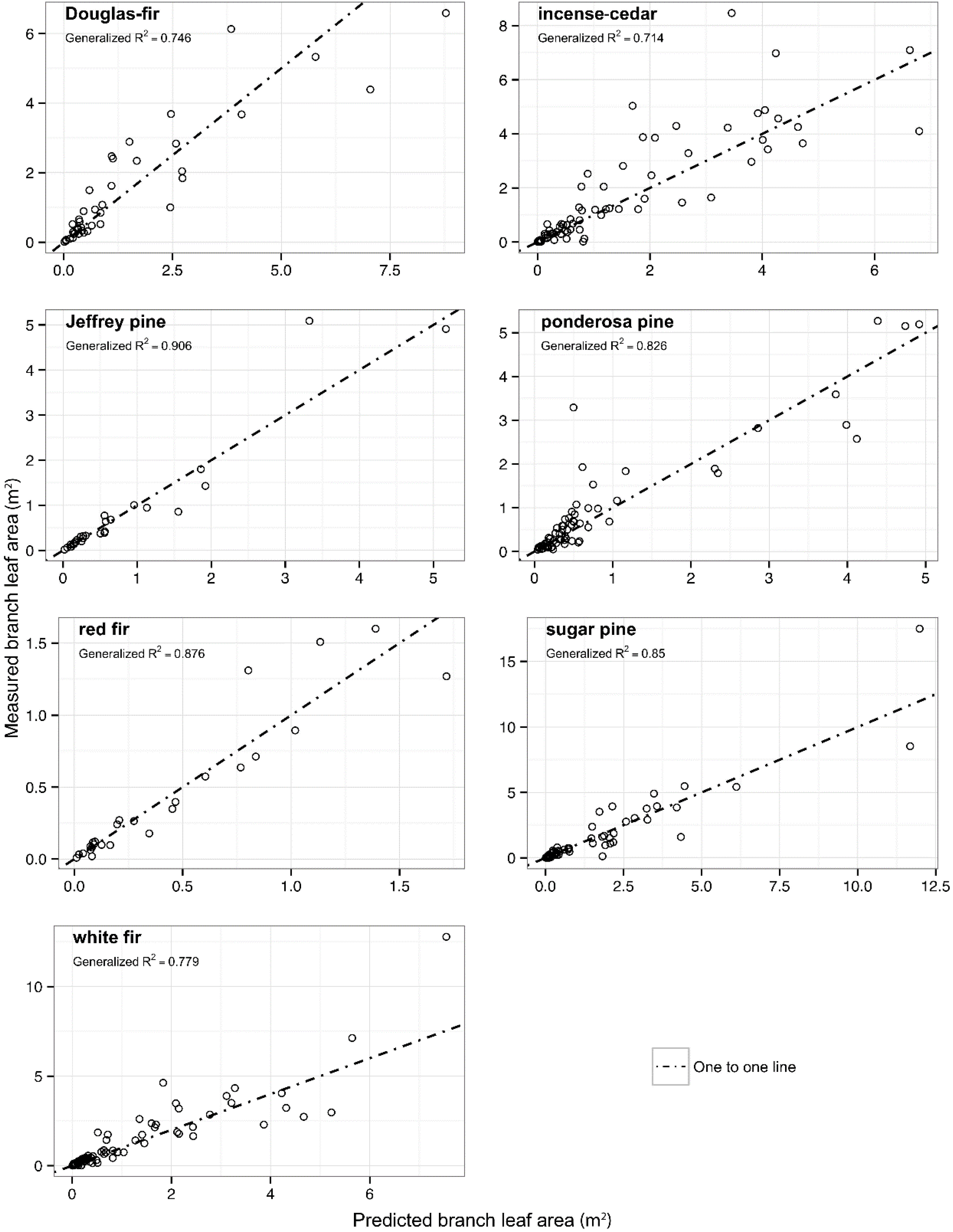
Figure 1 shows predicted branch leaf area
versus measured branch leaf area and generalized
R2 values for each species. Inclusion of a random effects parameter for site did not result in any significant improvements in model fit for any of the species. For red fir and Jeffrey pine, where only one site was sampled, the random effects tested were for individual trees, which also showed no significant impact on the branch leaf area model fit.
Table 5.
Summary of model parameter estimates for branch leaf area by species.
Table 5.
Summary of model parameter estimates for branch leaf area by species.
| Species | b1 | b2 | b3 | ΔAIC | n |
|---|
| Douglas-fir | LCR(1.17(0.27)) − RHFT·HDR(0.95(0.32)) | DHR(0.62(0.05)) | 1.74(0.14) | 1.52 | 44 |
| Incense-cedar | HDR·LCR(1.05(0.16)) | 1.53(0.10) − RHFT·LCR(1.38(0.24)) | −0.44(0.033) − RHFT(3.40 (0.36)) | −2.19 | 75 |
| Jeffrey pine | 0.53(0.06) − RDC(0.50(0.06)) | LCRM(0.44(0.06)) + RDC(0.97(0.11)) | 1.62(0.06) | −2.00 | 28 |
| Ponderosa pine | DC(0.20(0.08)) + I(0.15(0.04)) + S(0.08(0.02)) | 1.45(0.22) − LCR(0.83(0.33)) | 1.06(0.15) | −2.00 | 65 |
| Red fir | LCR(0.25(0.04)) | 1.22(0.083) | 1.57(0.08) | 0.90 | 27 |
| Sugar pine | HDR(0.49(0.08)) | 0.66(0.16) + LCR(0.56(0.27)) | LCR(2.13(0.16)) | −1.99 | 62 |
| White fir | HDR(0.33(0.04)) | 1.49(0.11) − RHFT·DHR(0.21(0.11)) | DHR(0.88(0.06)) | −2.00 | 77 |
The best-fit model for leaf area of crown portion was model 30 for all species except white fir where model 31 was a better fit. Parameter estimates including additional covariates can be found in
Table 6.
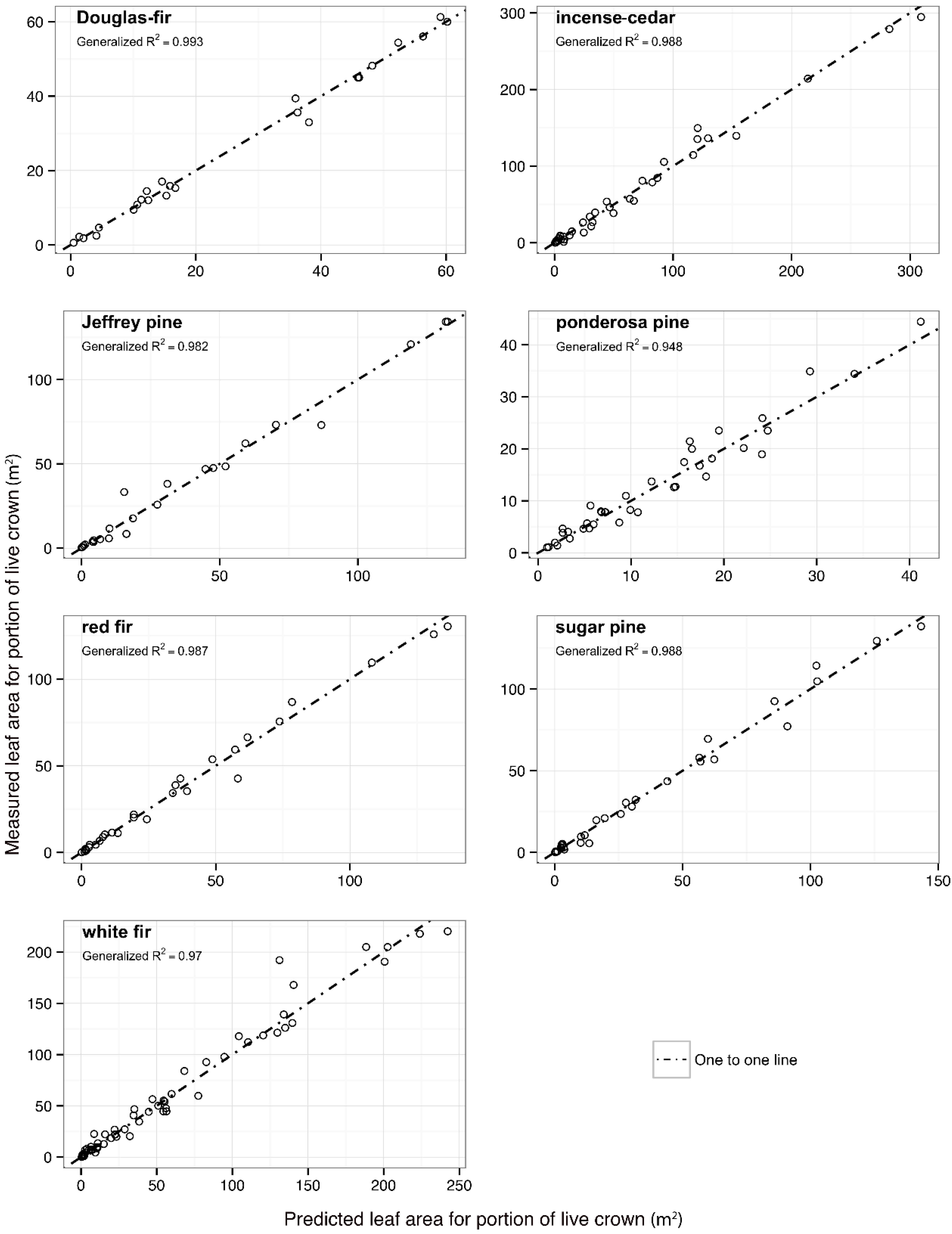
Figure 2 shows predicted leaf area of crown portion
versus measured leaf area and a generalized
R2 value for the final model for each species. There were no significant random effects related to the site for any of the species. Incense-cedar, ponderosa pine, and red fir all showed significant improvements in model fit using random effects at the tree level nested within site.
Table 6.
Summary of model parameter estimates for crown portion leaf area by species.
Table 6.
Summary of model parameter estimates for crown portion leaf area by species.
| Species | b1 | b2 | b3 | b4 | ΔAIC | n |
|---|
| Douglas-fir | 2.29(0.30) | 1.10 (0.19) | 0.17(0.03) + LCR(0.83 (0.06)) – RHFT(0.29 (0.04)) | NA | −3.00 | 24 |
| Incense-cedar | 1.00(0.17) | −2.70 (0.98) | 1.12(0.04) – LCR(0.60(0.06)) | NA | 11.40 * | 38 |
| Jeffrey pine | RHFT·DHR(1.36 (0.40)) | −2.27 (2.80) | RHFB(0.15(0.07)) | NA | −3.00 | 25 |
| Ponderosa pine | LCR·HDR(1.37 (0.21)) | −1.64 (0.79) | 0.55(0.05) + DHR(0.31(0.02)) – LCRM(0.52(0.04)) | NA | 22.82 * | 38 |
| Red fir | LCR(1.94 (0.28)) | T (1.38 (0.19) | −0.60(0.22) + LCR(1.36(0.25)) | NA | 11.14 * | 31 |
| Sugar pine | ILCR(0.32(0.05)) | −7.05 (3.48) | 0.67(0.05) + DHR(0.07(0.02)) | NA | −4.26 | 35 |
| White fir | ILCR (0.52(0.10)) | DHR (0.55(0.04)) | −DHR·T (1.81(0.38)) | 0.56(0.04) + LCR(0.32 (0.04)) − ITP(0.54(0.36)) | −3.00 | 62 |
Figure 1.
Measured branch leaf area as a function of predicted branch leaf area for seven conifer species. Generalized R2 are shown as well as one-to-one lines to indicate scatter around theoretical line of perfect fit.
Figure 1.
Measured branch leaf area as a function of predicted branch leaf area for seven conifer species. Generalized R2 are shown as well as one-to-one lines to indicate scatter around theoretical line of perfect fit.
Figure 2.
Measured leaf area for a crown portion as a function of predicted leaf area above a point in the crown for seven conifer species. Generalized R2 are shown as well as one-to-one lines to indicate scatter around the theoretical line of perfect fit.
Figure 2.
Measured leaf area for a crown portion as a function of predicted leaf area above a point in the crown for seven conifer species. Generalized R2 are shown as well as one-to-one lines to indicate scatter around the theoretical line of perfect fit.
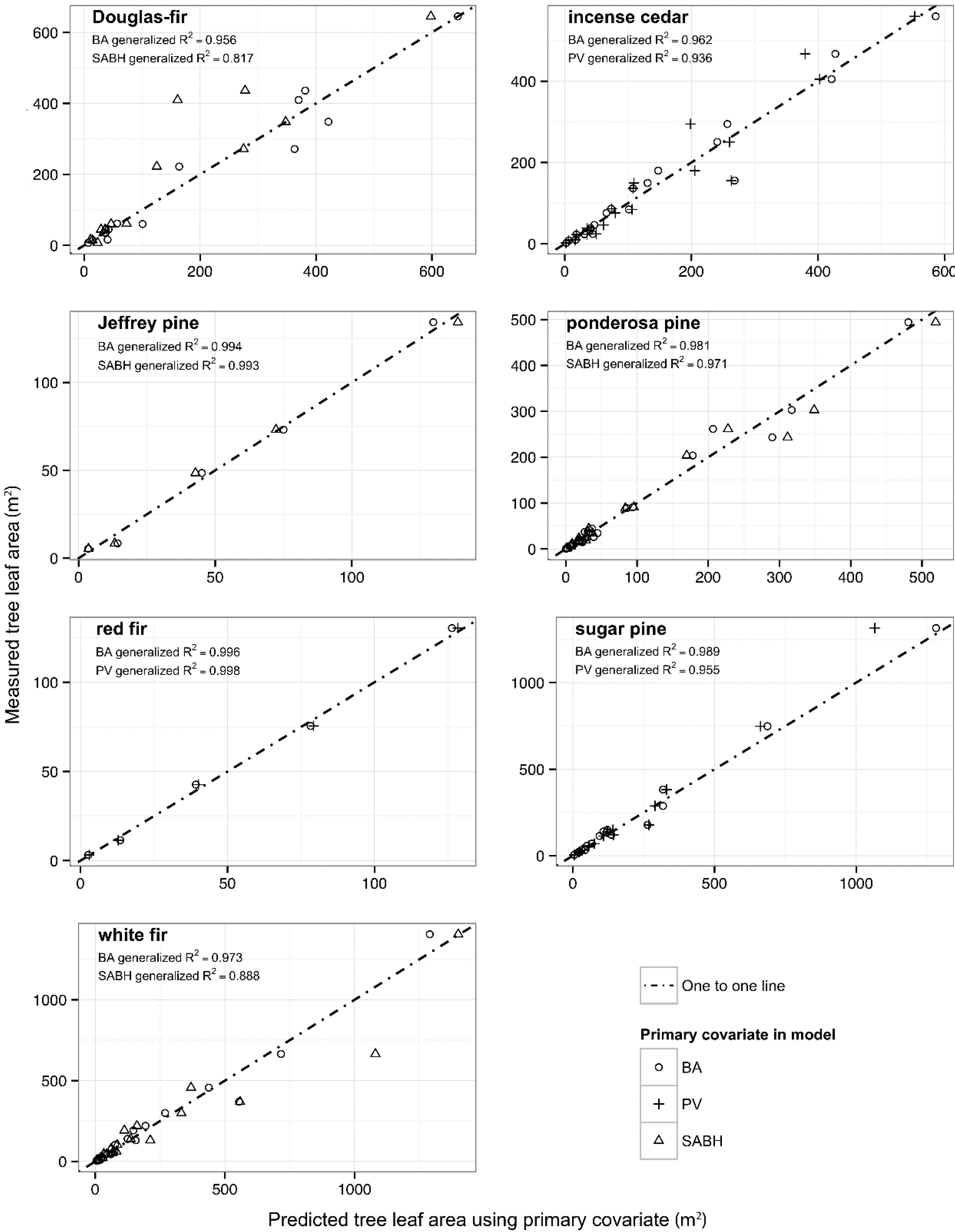
Figure 3.
Whole tree leaf area as a function of predicted leaf area from two best-fit functions for seven conifer species. Generalized R2 model fits for top two primary covariates are shown as well one-to-one lines to indicate scatter around theroetical line of perfect fit.
Figure 3.
Whole tree leaf area as a function of predicted leaf area from two best-fit functions for seven conifer species. Generalized R2 model fits for top two primary covariates are shown as well one-to-one lines to indicate scatter around theroetical line of perfect fit.
The best-fit prediction model for whole tree leaf area was model 19 with basal area as the primary covariate for Douglas-fir, incense-cedar, Jeffrey pine, and red fir. White fir and ponderosa pine had the lowest AIC fits with model 12 and cross-sectional sapwood area as the primary covariate. The best-fit model for sugar pine was model 13 with the parabolic volume as the primary covariate. Parameter estimates for all species and best-fit models including additional covariates can be found in
Table 7. Model 19 fits are also included for each species in
Table 7 as this model had the best overall performance.
Figure 3 shows data points for predicted whole tree leaf area for model 19 with basal area as primary covariate along with either the lowest, or second lowest model by AIC. Generalized
R2 values for each species model and primary covariate are included in
Figure 3. For all models tested, there was no significant improvement in model fit when random effects for site were included. Testing for differences in fixed effect parameter estimates related to sampling procedure categorical variables showed a significant difference between the two destructive sampling categories for ponderosa pine (D2D
vs. D1) for both parameters in the model (
Table 8). Testing for differences between fixed effects for D1 and D2 resulted in no significant differences for any of the species tested (
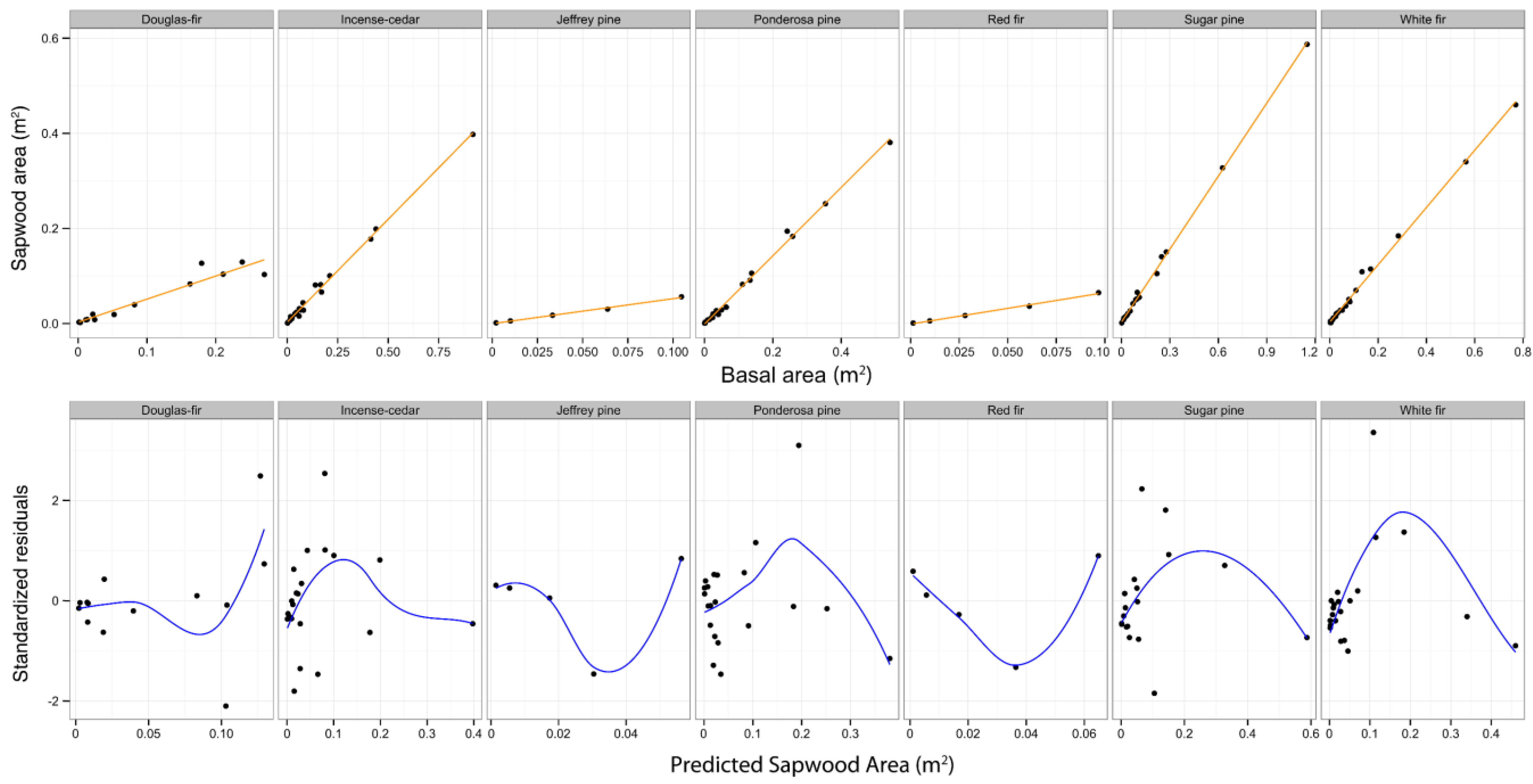
Table 8). A linear regression of sapwood area
versus basal area and the residuals from that regression are shown in
Figure 4. A LOESS (locally weighted scatterplot smoothing) regression was performed on the residuals against basal area using the R “stats” package version 3.3.0 [
47], to determine if a pattern existed within the residuals of the linear regression (
Figure 4).
Figure 4.
Linear regressions of cross sectional sapwood area (m2) at breast height against basal area are shown in the top row for each species. Standardized residuals from the linear regressions are plotted against predicted sapwood area (m2) in the bottom row. LOESS regressions of the standardized residuals against predicted sapwood area are also shown in the bottom row.
Table 7.
Summary of parameter estimates for whole tree leaf area prediction models by species.
Table 7.
Summary of parameter estimates for whole tree leaf area prediction models by species.
| Primary Covariate | Species | Model | b1 | b2 | b3 | AIC | n | AIC Rank |
|---|
| BA | Douglas-fir | 19 | DHR(0.6823(0.0054)) | 0.7194(0.0085) + ICI(0.0040(0.0002)) | NA | 118.9 | 14 | 1 |
| SA | Douglas-fir | 12 | DHR(0.3059(0.0306)) | 1.7298 (0.1087) | NA | 137.9 | 14 | 3 |
| BA | Incense-cedar | 19 | BHCR(0.1703(0.0488)) | 0.8147(0.0466) + HDR (0.2590(0.1273)) + CI(0.7668 (0.2365)) | NA | 188.3 | 21 | 1 |
| SA | Incense-cedar | 21 | 0.2803(0.0288) | 2790.0910(1155.5231) | −0.9359 (0.7185) | 206.2 | 21 | 6 |
| BA | Jeffrey pine* | 19 | 0.2397(0.1203) | 0.9111(0.0806) – CI(0.4480 (0.1055)) | NA | 186.7 | 26 | 1 |
| SA | Jeffrey pine* | 12 | 0.2485(0.0213) – CI(0.1652 (0.0424)) | 0.1166(0.1246) | NA | 192.5 | 26 | 3 |
| SA | Ponderosa pine | 12 | DHR(0.0641 (0.0045)) | 0.3367(0.1232) – LCHLCR(0.4174(0.1247)) | NA | 142.1 | 21 | 1 |
| BA | Ponderosa pine | 19 | 0.0658(0.0151) – CI(0.0548 (0.0186)) | 1.0178(0.0346) + ICI(0.0034 (0.0012)) | NA | 145.8 | 21 | 2 |
| BA | Red fir* | 19 | 0.1410(0.0307) | 0.8093(0.0383) + BHCR(0.1931 (0.0447)) | NA | 225.3 | 26 | 1 |
| SA | Red fir* | 26 | 0.1949(0.0433) + DHR·BHCR(0.0544(0.0196)) | NA | NA | 231.8 | 26 | 4 |
| PV | Sugar pine | 13 | 169.3656(5.7259) | 0.7033(0.0084) | LCR (1.3863 (0.0722)) | 132.5 | 18 | 1 |
| BA | Sugar pine | 19 | 0.0832(0.0034) + ICP(0.0344(0.0008)) | 0.9801(0.0095) | NA | 136.7 | 18 | 2 |
| SA | Sugar pine | 12 | 0.2165(0.0170) + CI(0.4969(0.1541)) | LCR(0.5871 (0.1892)) | NA | 141.2 | 18 | 4 |
| SA | White fir | 12 | LCR(0.3460(0.0122)) | −ILCR(0.4986 (0.0495)) | NA | 192.6 | 21 | 1 |
| BA | White fir | 19 | ILP(0.1158(0.0280)) | 0.8792(0.0494) + LCR(0.1885 (0.0639)) | NA | 193.8 | 21 | 2 |
Table 8.
Comparisons between fixed effect parameter estimates for D1 versus all other dataset categories (D2, D2C, and D2D).
Table 8.
Comparisons between fixed effect parameter estimates for D1 versus all other dataset categories (D2, D2C, and D2D).
| Species | Fixed Effect Compared | Difference from D1 | Standard Error | Degrees of Freedom | t-Value | p-Value |
|---|
| Douglas-fir | D2-b1 | 0.0558 | 0.0954 | 9 | 0.585 | 0.573 |
| Douglas-fir | D2-b2 | 0.0066 | 0.0183 | 9 | 0.358 | 0.729 |
| Douglas-fir | D2C-b1 | 0.0530 | 0.8383 | 5 | 0.063 | 0.952 |
| Douglas-fir | D2C-b2 | 0.0410 | 0.0241 | 9 | 1.702 | 0.123 |
| Douglas-fir | D2D-b1 | −0.3012 | 0.1619 | 5 | −1.860 | 0.122 |
| Douglas-fir | D2D-b2 | 0.0063 | 0.0140 | 9 | 0.452 | 0.662 |
| Incense-cedar | D2-b1 | −0.0023 | 0.0160 | 15 | −0.144 | 0.887 |
| Incense-cedar | D2-b2 | −0.0048 | 0.0190 | 16 | −0.251 | 0.805 |
| Incense-cedar | D2C-b1 | −0.0020 | 0.0209 | 9 | −0.095 | 0.926 |
| Incense-cedar | D2C-b2 | 0.0013 | 0.0247 | 15 | 0.052 | 0.959 |
| Incense-cedar | D2D-b1 | −0.0034 | 0.0194 | 9 | −0.178 | 0.863 |
| Incense-cedar | D2D-b2 | 0.0077 | 0.0254 | 15 | 0.302 | 0.767 |
| Ponderosa pine | D2-b1 | 0.0060 | 0.0068 | 12 | 0.894 | 0.389 |
| Ponderosa pine | D2-b2 | 0.0068 | 0.0166 | 12 | 0.412 | 0.688 |
| Ponderosa pine | D2C-b1 | 0.0133 | 0.0097 | 11 | 1.365 | 0.199 |
| Ponderosa pine | D2C-b2 | 0.0218 | 0.0138 | 11 | 1.583 | 0.142 |
| Ponderosa pine | D2D-b1 | −0.0185 | 0.0055 | 11 | −3.349 | 0.006 * |
| Ponderosa pine | D2D-b2 | −0.0444 | 0.0160 | 11 | −2.773 | 0.018 * |
| Sugar pine | D2-b1 | 0.0128 | 0.0113 | 9 | 1.132 | 0.287 |
| Sugar pine | D2-b2 | 0.0135 | 0.0116 | 9 | 1.161 | 0.276 |
| Sugar pine | D2C-b1 | 0.0051 | 0.0393 | 8 | 0.130 | 0.900 |
| Sugar pine | D2C-b2 | 0.0015 | 0.0322 | 8 | 0.047 | 0.964 |
| Sugar pine | D2D-b1 | −0.0149 | 0.0131 | 8 | −1.139 | 0.288 |
| Sugar pine | D2D-b2 | −0.0149 | 0.0125 | 8 | −1.195 | 0.266 |
| White fir | D2-b1 | 0.0385 | 0.0362 | 11 | 1.064 | 0.310 |
| White fir | D2-b2 | 0.0147 | 0.0187 | 12 | 0.788 | 0.446 |
| White fir | D2C-b1 | 0.1471 | 0.2464 | 15 | 0.597 | 0.560 |
| White fir | D2C-b2 | −0.0033 | 0.0262 | 16 | −0.127 | 0.901 |
| White fir | D2D-b1 | −0.1594 | 0.1172 | 15 | −1.361 | 0.194 |
| White fir | D2D-b2 | −0.0137 | 0.0214 | 16 | −0.641 | 0.531 |
4. Discussion
The overall performance of model 19 with basal area as the primary covariate was impressive given that there is a weaker biological connection between basal area and leaf area as compared to sapwood cross-sectional area and leaf area of larger trees. This result does not refute the pipe model theory; instead, it demonstrates that alternate models can be more effective at predicting leaf area without the functional basis of the pipe model theory. These alternative model forms also avoid the need for variables, such as sapwood cross-sectional areas, that are both difficult and expensive to obtain. However, models with sapwood cross-sectional area also performed well (
Table 7). Model 12 is the only model taken from existing literature [
41] to have outperformed model 19 but the difference in model fits was only significant for ponderosa pine. The strong performance of model 19 across all species recommends it for whole tree leaf area prediction within the modeled Sierra Nevada conifers.
The relationship between sapwood cross-sectional area and basal area of individual trees is nonlinear as shown by the pattern of the standardized residuals in
Figure 4. However, this relationship could be modeled efficiently with nonlinear functions of basal area. Model 19 creates a sigmoid fit at very small basal areas and transitions to a power fit as diameter increases. The curvature of this model likely tracks the nonlinear relationship between sapwood area and basal area. A nonlinear relationship is consistent with the development of heartwood within tree stems over time. At small diameters, sapwood makes up all, or nearly all, of the inside bark basal area. However, as trees grow sapwood area as a proportion of inside bark basal area gradually declines as sapwood is converted into heartwood. This reduction in sapwood proportion with increasing diameters precludes a consistent linear relationship between sapwood area and basal area. It is possible that model 19 is tracking the relationship between functional sapwood area and basal area, which could explain how basal area performs better than sapwood area in predicting leaf area despite basal areas weaker biological connection to leaf area. It is also possible that sapwood area measurements were simply less accurate than basal area measurements and that inaccuracy introduced additional noise in the sapwood area leaf area relationship.
Red fir and Jeffrey pine demonstrate apparently different patterns in their residuals from the other species. This difference in residual patterns is most easily attributed to the smaller range of tree sizes represented in the data for those two species. Across all species, however, very similar residual patterns are apparent within similar size ranges. For example, the average of the residuals is negative or zero at basal area values below 0.04 m
2, positive around 0.15 m
2, and negative again around 0.4 m
2. Residuals from a linear regression should be evenly distributed around 0 across predicted values. The curvature of the LOESS regression demonstrates that the sapwood and basal area relationship is nonlinear, and demonstrates the similarity in the general residual pattern between species. The appearance of a potentially linear fit to the data displayed in the upper row of
Figure 4 is attributable to the large range in basal area values that occur between sampled trees, thereby visually stretching the data points out far enough that, on cursory inspection, a linear fit appears to be suitable. A quick review of standardized residuals plotted against the fitted values is suggested to check for linearity [
48], and in this case the residuals show departures from a linear relationship.
The components of model 19 have somewhat intuitive interpretations where parameter b
1 is a proportion of the functional form; parameter b
2 is the power law rate parameter; and the exponential term (1 − e
−X) provides a brake on the rate (power) of increase at small basal areas. Indicators of competition experienced by the sampled trees, specifically LCR, BHCR, ICI, HDR and CI have significant influence on the b
2 and to a lesser extent the b
1 parameter for most of the species analyzed (see
Table 4 for descriptions of covariates). The influence of these covariates on the b
1 and b
2 parameters vary from the original pipe model theory [
20] which assumed a linear relationship between leaf area and sapwood area, and supports more recent research demonstrating that the leaf area—sapwood area relationship is not necessarily linear [
49,
50]. The influence of these covariates on the leaf area—sapwood area relationship is most directly interpreted in the models with sapwood area as the primary covariate. For most of the sapwood area models there were significant effects on parameter estimates from covariates that represent competition such as LCR, DHR and CI (
Table 7).
Improvement in the relationship between sapwood area and leaf area due to the addition of competition related covariates indicates the potential for competition to influence the sapwood area to leaf area ratio (
Table 7). The improved model fit from the addition of competition related covariates could reflect the effect of shade on the evaporative stress on understory foliage and shaded foliage within codominant and intermediate trees. Evaporative stress has been shown to significantly influence the sapwood area to leaf area relationship [
24,
51,
52], as does stand density [
53,
54]. To make this inference stronger, the analysis would have to be rerun with competition indexes developed from measurements of the trees surrounding the study trees. This study did not measure all trees around the selected study trees making this analysis impossible. Alternatively, segmenting the study trees by canopy class would have resulted in too few individuals in each class to develop meaningful models.
The lack of significant site level random effects on any of the leaf area prediction model fits suggests that the underlying models are accounting for most of the variation due to growing environment and growth history. This is likely due to the covariates related to growing conditions of the study trees. For instance, the inclusion of height: diameter ratios may account for some stand density influence as this metric is affected by competition. This inference does not hold for Jeffrey pine or Red fir as those species only had one site sampled and therefore had no site level random effects. No relationship between species shade tolerance and the modeled leaf area relationships were detected.
The lack of significant fixed effects for the sampling categories (D1 and D2) using model 19 with basal area as the primary covariate indicated that the leaf area data gathered by these procedures can be combined for the purposes of model fitting (
Table 8). As both sampling procedures are designed to estimate leaf area and both procedures use weight of foliage as one of the predictors of total leaf area it was not surprising that there was no significant influence of sampling category on the model parameter estimates, however, this lack of difference was important in justifying the combination of leaf area data from both categories in the final model fits for whole tree leaf area. The significant differences in parameter estimates between the two destructive sampling procedures (D1 and D2D) in ponderosa pine shown in
Table 8 are likely due to the fact that destructively sampled trees in D1 were larger on average than trees in the D2D subcategory. Overall the lack of significant differences in parameter estimates related to sampling category and the lack of significant random effects associated with site suggests that these models are accurately estimating the underlying relationship between whole tree leaf area and basal area for each species.
The strong potential to predict leaf area of a portion of the crown is demonstrated by the strong coincidence of the data to the one to one line, a reference line indicating “perfect” predictive power for the given leaf area model relative to the measured data (
Figure 1,
Figure 2 and
Figure 3). Interestingly, the best-fit models for leaf area of crown portion had parabolic sapwood volume (model 30 and 31) as the primary covariate, although this was not a significant covariate for whole tree leaf area. This suggests that sapwood area is a stronger predictive covariate for measurements below the live crown while parabolic sapwood volume, an estimate of total sapwood volume, appears to be a stronger predictor of leaf area above a point in the live crown. This may be related to the fact that sapwood volume below live crown is not directly related to total leaf area while sapwood volume in the live crown is related to the leaf area above it. It may be that sapwood volume is better able to account for changes in vapor pressure related to changing canopy position of foliage within the tree. Parameter b
3 was most consistently affected by the addition of covariates (
Table 6). Each species showed an improved model fit by the addition of covariates to this parameter while none of the other parameters showed as consistent a response. Parameter b
3 in these models acts as a rate parameter on the relationship between parabolic sapwood volume and leaf area. This parameter is similar to the rate parameter in the whole tree models as it is influenced by LCR, DHR and other covariates related to competition. Parameter b
1 is similar in effect to b
1 from the whole tree models in that it represents a proportion of the functional form. As in the case of the whole tree models this parameter is also significantly influenced by competition related covariates.
Predicting leaf area above a point in the live crown through non-destructive procedures is useful for research of leaf area allometries across a range of diameters as many large trees cannot be felled due to the importance of large trees as wildlife habitat, lost timber value, cost of hiring professional fellers,
etc. It was due, in part, to these restrictions on cutting trees above a certain size that we explored non-destructive sampling procedures. Similar approaches have been used to estimate foliar mass for endangered trees that cannot be cut down for legal reasons [
55]; however, our utilization of destructively sampled trees for calibration likely added to the strong performance of the final model.
The models with the lowest generalized R2 were the branch leaf area prediction models. This was expected as every branch on sampled trees, including internode branches, was a potential sample branch. Internode branches are more likely to be in the shade of other branches, which likely alters the branch cross-sectional area to leaf area relationship as shading would reduce evaporation rates while leaf stomata are open, thereby reducing the size of “pipe” necessary to support a given amount of leaf area. There is also the potential for increased variation due to the inclusion of branches shaded by canopy competitors, or branches facing north versus south. Despite these sources of error, the modeling procedures produced reasonable model fits for each of the seven species. Given the high degree of variation in live crown length, branch sizes, site competition and site quality, it was surprising that this variation in branch leaf area estimates did not lead to greater variation in the leaf area prediction models for whole tree and crown portion. This is even more surprising given that the primary covariates—parabolic sapwood volume and basal area—are not directly linked to branch size or distribution.


