Article

Sparse Density, Leaf-Off Airborne Laser Scanning Data in Aboveground Biomass Component Prediction

1
Department of Forest Sciences, University of Helsinki, Helsinki FI-00014, Finland
2
Centre of Excellence in Laser Scanning Research, Finnish Geodetic Institute, Masala FI-02431, Finland
3
School of Forest Sciences, University of Eastern Finland, Joensuu FI-80101, Finland
4
Department of Remote Sensing and Photogrammetry, Finnish Geodetic Institute, Masala FI-02431, Finland
5
Department of Real Estate, Planning and Geoinformatics, Aalto University, Aalto FI-00076, Finland
6
Civil engineering and building services, Helsinki Metropolia, University of Applied Sciences, Helsinki FI-00079, Finland
7
Department of Geography and Geology, University of Turku, Turku FI-20014, Finland
*
Author to whom correspondence should be addressed.
Forests 2015, 6(6), 1839-1857; https://doi.org/10.3390/f6061839
Submission received: 14 April 2015 / Revised: 5 May 2015 / Accepted: 25 May 2015 / Published: 28 May 2015

Abstract

:
The demand for cost-efficient forest aboveground biomass (AGB) prediction methods is growing worldwide. The National Land Survey of Finland (NLS) began collecting airborne laser scanning (ALS) data throughout Finland in 2008 to provide a new high-detailed terrain elevation model. Similar data sets are being collected in an increasing number of countries worldwide. These data sets offer great potential in forest mapping related applications. The objectives of our study were (i) to evaluate the AGB component prediction accuracy at a resolution of 300 m2 using sparse density, leaf-off ALS data (collected by NLS) derived metrics as predictor variables; (ii) to compare prediction accuracies with existing large-scale forest mapping techniques (Multi-source National Forest Inventory, MS-NFI) based on Landsat TM satellite imagery; and (iii) to evaluate the accuracy and effect of canopy height model (CHM) derived metrics on AGB component prediction when ALS data were acquired with multiple sensors and varying scanning parameters. Results showed that ALS point metrics can be used to predict component AGBs with an accuracy of 29.7%–48.3%. AGB prediction accuracy was slightly improved using CHM-derived metrics but CHM metrics had a more clear effect on the estimated bias. Compared to the MS-NFI, the prediction accuracy was considerably higher, which was caused by differences in the remote sensing data utilized.

1. Introduction

Accurate forest biomass mapping methods are required globally and could be utilized e.g., for predicting forest aboveground biomass (AGB), bioenergy potential and carbon stock. The use of forest-based bioenergy is also increasing and will play a major role in the bioenergy sector in the near future. At the moment, a typical approach to mapping AGB over large areas is based on generalizing field sample plot measurements using coarse- or medium-resolution remote sensing (RS) data and other numeric map data. For sample plots, the amount of AGB is estimated using local allometric models (e.g., [1,2]). This approach, referred to as Multi-Source National Forest Inventory (MS-NFI), was first introduced and tested in Finland in the early 1990s (e.g., [3]) and is nowadays routinely used in the Nordic countries to generate biomass maps for various purposes [3].
Forest management practices, e.g., in Finland, are based on intensive, small-scale forestry, which results in mosaic-like forest structures and stand sizes of approximately 2 ha on average. Mapping AGB over larger areas under such land use or vegetation patterns is challenging based on medium- or coarse-resolution RS data with pixel sizes varying from 30 m × 30 m (e.g., Landsat 7) to 250 m × 250 m (e.g., MODIS). Previous studies have shown that the mismatch between field measurement data, an individual pixel of satellite data [4] and the scarcity of available field data are the main challenges in forest attribute prediction. Coarse pixel size in the RS data results in mixed pixels on stand boundaries and thus an inaccurate description of the vegetation structure variability especially when looking at relatively small areas (e.g., forest stands of 1–3 hectares or field-measured sample plots). For example, Tuominen et al. [5] used Landsat 5 TM imagery with a resampled pixel size of 25 m × 25 m to predict total volume and AGB. Estimated root-mean-squared error (RMSE) of the total volume and AGB varied between 65.1% and 73.1% of the mean plot-level reference values. Such accuracy levels are not acceptable for detailed AGB mapping, which is required e.g., in bioenergy harvesting. More detailed methods are therefore needed for AGB mapping, especially at the local (plot or pixel) level.
Airborne laser scanning (ALS) is a three-dimensional (3D) measurement technique, which is becoming increasingly popular in forest resource mapping. ALS data can be used to predict a variety of forest inventory attributes with a high level of accuracy [6,7] due to its capability of describing 3D vegetation structure. ALS has two main approaches for estimating forest information: an area-based approach (ABA, [6]) and individual tree detection (ITD, [8]). Forest AGB prediction with laser scanning techniques has previously been studied at varying levels, from single trees (e.g., [9,10,11,12,13,14]) to larger areas. Recent overviews are provided by Zolkos et al. [15] and Popescu and Hauglin [16].
The coefficient of determination values (R2) between predicted AGB and laser-derived metrics have previously varied between 0.32 and 0.92 depending on, e.g., tree species and development classes. Combined small-footprint ALS and multispectral airborne data were used in Popescu et al. [17] to predict AGB in deciduous and pine (Pinus L.) forests at a resolution of 168 m2. The maximum R2 values were 0.32 for deciduous and 0.82 for pine dominated sample plots. Aardt et al. [18] improved the R2 values for deciduous trees to 0.58 using ALS point height metrics as predictors in a per-segment prediction of AGB. The highest R2 values were reported by Næsset [19], who used regression methods to predict AGB for 143 sample plots (size of 300–400 m2) in young and mature coniferous forests. The regression models explained 92% of the AGB variability for all forest types.
Latifi et al. [20] compared different nearest neighbor (NN) and random forest (RF) techniques for the prediction of volume and AGB in southwestern Germany, with the target areas for which the AGB values were predicted varying from 13 m2 to 452 m2. They concluded that the RF method was superior to other NN methods. ABA accuracy depends highly on the coverage of different forest structures within the training data and the prediction technique used [7]. According to Fassnacht et al. [21] the data type (RS) had the highest impact on the AGB prediction accuracy. Prediction technique was seen as the second most important factor. Fassnacht et al. [21] also concluded that increasing the sample size of the modeling data did not effectively improve the AGB prediction accuracy. Stepper et al. [22] confirmed this conclusion and reported that decreasing the sample size from 1875 plots to 226 plots had a minimal effect on the model performance. Traditionally the required training data for the ABA is measured in the field, which is costly, especially in remote areas. Vastaranta et al. [23] used ITD to replace field measurements required for the ABA. This method was further tested for AGB prediction in Kankare et al. [24]. The AGB prediction RMSEs varied between 23.0 and 32.3 tons per ha. Tuominen and Haapanen [25] reported similar or slightly higher prediction accuracies using a combination of ALS and digital aerial photograph-derived metrics.
The National Land Survey of Finland (NLS) began collecting ALS data over the entire area of Finland in 2008 to provide a new national-level elevation model. The data are available free of charge from their data services. As corresponding data are also increasingly available in several other countries, e.g., Sweden, Italy, Spain, USA, Netherlands and England, (e.g., [26,27,28]), these data are expected to have a great potential and a wide variety of possible applications in forestry and especially in forest biomass mapping and monitoring. Although the data are essentially acquired for ground elevation modeling, Nord-Larsen and Schumacher [29] and Villikka et al. [30] verified the suitability of these data also for forest attribute prediction. However, they did not compare the obtained accuracies with any existing inventories such as the MS-NFI. To better justify bringing a new method to operational forestry, it should be shown to yield at least at a similar level of accuracy as the presently used inventory methods. Overall, no studies reporting component biomass prediction accuracies based on sparse density, leaf-off ALS data currently exist in the literature.
The main objective of our study was thus to evaluate the accuracy of predicting AGB and its components (stem, living branch and canopy biomass) using sparse density, leaf-off ALS data collected essentially for elevation modeling. The ALS metrics were derived at plot-level (300 m2) and tested as predictor variables to predict AGB components. Results were compared to the Multi-Source National Forest Inventory (MS-NFI, ©Finnish Forest Research Institute 2012) AGB estimates. Similar datasets are being collected in several countries worldwide, and the comparison is therefore seen as important towards detailed large-scale forest resource mapping applications. Since the ALS data were acquired with multiple sensors and varying scanning parameters, we also derived the corresponding metrics from a canopy height model (CHM) and tested this type of feature extraction as an alternative strategy to eliminate the sensor effects. Our detailed objectives were: (1) to evaluate the accuracy of the AGB component prediction at a resolution of 300 m2; (2) to compare AGB prediction accuracy to an existing approach of predicting AGB over large areas; and (3) to evaluate the accuracy and effects of the CHM derived metrics on the AGB component prediction accuracy.

2. Materials and Methods

2.1. Study Area and Field Measurements

Our study area is located at Evo, Finland (61.19° N, 25.11° E). The area belongs to the southern boreal forest zone and a broad mixture of forest stands, varying from natural to intensively managed, is available. Scots pine (Pinus sylvestris L.) and Norway spruce (Picea abies (L.) H. Karst.) are the dominant tree species in the study area, contributing 78.2% of the total volume according to the field inventory data. The original field data comprised 368 circular plots of radius 9.77 m (300 m2). All trees with a diameter-at-breast-height (dbh) larger than 5 cm were measured within this radius. The following tree variables were measured in the field: species, canopy layer (dominant or sub), dbh and height. Field plot sampling was based on the prestratification (see [24]) of existing stand inventory data to distribute plots over various site types, tree species and stand development classes. In total, 40 strata were used to distribute the initial sample plots to different species-specific volume stratums and site types (mineral/peatland and site fertility class). The field plots were located with a GEOXM 2005 global positioning system (GPS) device (Trimble Navigation Ltd., Sunnyvale, CA, USA), and the locations were postprocessed with local base station data resulting in an accuracy of approximately 0.6 m.
AGB was estimated for single trees using allometric models and field-measured species, dbh and height as predictors [1,2]. Separate models were used for Scots pine, Norway spruce and birch (Betula pendula Roth and Betula pubenscens Ehrh.). The following AGB components were estimated: total (TotalB), stem (StemB), living branch (LivB) and canopy (CanopyB). The basic statistics can be found in Table 1. Plot-level (300 m2) AGB components were then summed from individual tree estimates within each sample plots.
The original field sample plot data were covered by two different sensors (see Section 2.2.), from which 255 sample plots were covered by Leica (“Leica-plots”) and 113 by Optech (“Optech-plots”). To minimize the effect of sample plot data variability to the accuracy evaluations of the AGB predictions, the amount of sample plots covered by the sensors was equalized. The reduction of the Leica-plots was done according to the following procedure: (1) the reference biomass frequencies were calculated in classes of 20 tons per ha; and (2) an amount of Leica-plots corresponding to the amount of Optech-plots was selected in random in each class and retained for the analyses. The final data set for the AGB predictions and accuracy evaluations consisted of 226 sample plots (113 per sensor).
Table 1. Descriptive statistics of measured forest attributes.
MINMEANMAXSTDEV
Dgm, mm77.7227.9558.579.2
Hgm, m5.119.031.05.2
V, m3/ha4.7205.9653.6113.5
N, 1/ha133.01007.83001.0599.3
TotalB, t/ha2.8104.8302.853.1
StemB, t/ha1.374.3208.938.2
CanopyB, t/ha0.824.188.213.9
LivB, t/ha0.614.040.67.2

2.2. Airborne Laser Scanning Data

NLS conducted the ALS campaign in 2012 in the study area as part of their mission to create a new elevation model for Finland. The study area was covered using two different scanner systems: the northern part with Leica ALS50 scanner and the southern part with Optech ALTM GEMINI. The flying altitudes were 2200 m and 1830 m and the pulse densities approximately 0.8 and 0.7 pulses per m2 with Leica and Optech scanners, respectively.
ALS data sets were classified into ground and non-ground points by the data provider. A digital terrain model (DTM) was formed, using the classified ground points and searching for the lowest point inside each pixel. DTM pixel size was set at 1 m × 1 m. A digital surface model (DSM) was then created from the remaining vegetation points, by searching for the highest point within each pixel. DSM pixel size was also 1 m. The empty pixels (without any laser points) were filled using Terrascan’s Fill Gaps parameter during surface model creation. The parameter was set to 5. The aboveground laser heights (normalized height or CHM) were calculated by subtracting DTM from DSM.

Metric Extraction

Descriptive laser metrics for the sample plots were derived (1) from classified ALS point clouds and (2) from the CHM pixels. Individual pixel values (x, y, z and height from ground) within the sample plot were utilized in similar manner than the ALS point cloud in metric extraction. The most common ALS-based predictor variables (cf. [31]), i.e., the maximum, the mean and standard deviation of the height values; coefficient of variation of height values; the proportion of echoes or CHM pixels above 2 m height value in the 5th, 10th, 20th, …, 90th, and 95th percentiles; and the corresponding proportional densities of the ALS-based canopy height distribution; were calculated according to Korhonen et al. [32].

2.3. Biomass Prediction and Accuracy Assessment

TotalB and biomass components were predicted by means of ALS point or CHM-derived metrics using the NN approach. The sample plot data were divided into testing and training sets using the following procedure. The sample plot data were first divided into three subsets using the following dbh limits: (1) Young, dbh was lower than or equal to 15 cm; (2) Mature, dbh was larger than 15 but smaller than or equal to 25 cm; and (3) Old, dbh was larger than 25 cm. The test and training data sets were then composed by selecting sample plots from each subset (young, mature and old) randomly and in equal portions compared to the reference subsets. One hundred twenty-six sample plots were used in training and 100 in validation of the prediction accuracies. The estimated AGBs for the field measurements were used as the response variable (y value), and ALS point or CHM-derived metrics were used as predictors (x values). Random Forest (RF) was applied in the search for nearest neighbors due to robustness and flexibility in forest-variable prediction compared to other nearest neighbor distance measures [33]. The nearest neighbors are defined based on the observational probability of ending up in the same terminal node in classification [34]. The distance measure for the nearest neighbor search is defined as one minus the portion of the trees, where the portion of the trees is calculated based on the number of target observations compared to reference observations in the same terminal node, this being further explained by Crookston and Finley [34]. A total of 1000 regression trees were fitted in each RF run. The R statistical computing environment [35] and yaImpute library [34] were applied in the RF predictions. To further evaluate and compare the AGB component prediction accuracies with the ALS point or CHM-derived metrics as predictor variables, the NN predictions were repeated 500 times to assess the model performance and the effect of training and validation data composition. The number of iterations (500) was selected based on analyzing the estimated bias% and RMSE% of totalB with varying number of iterations from 50 to 500 with an interval of 50 (see Appendix B). The number of neighbors (k) in NN predictions was set to six based on analyzing the acquired prediction results using various k-values (see Appendix A).
The effect of two sensors used in data collection was also tested by dividing the sample plot data into training and test sets using scanning equipment. Optech ALTM Gemini and Leica ALS50 covered 113 and 113 sample plots, respectively (see for more details in Section 2.1). Accuracies were assessed by estimating biases and RMSEs of the predictions:
B i a s ^ = i = 1 n ( y i y ^ i ) n
M S E = i = 1 n ( y i y ^ i ) 2 n
where n is the number of observations, yi the value estimated from the field data for observation i and y ^ i . the predicted value for observation i. A paired t-test was used to test the significance of the mean difference between yi and y ^ i .

2.4. Biomass Estimates Based on the Multi-Source National Forest Inventory

MS-NFI estimates were used to provide benchmark accuracies for the ALS data analyses (Section 2.3). The estimates were based on an operational, nationwide method, in which the NFI sample plots (measured in 2007–2011) and satellite images (2009–2011) were used with a method called “improved k-Nearest Neighbor” [3,36].
The MS-NFI raster maps (Finnish Forest Research Institute 2012©) represent the 2011 forest biomasses estimated to a grid of 20 m × 20 m resolution. The following AGB-related raster maps were accessed (11 March 2014) by tree species (Norway spruce, Scots pine and deciduous trees): (1) stem and bark, (2) living branches, (3) dead branches, and (4) foliage (needles or leaves). TotalB raster was created by calculating the sum of these components. The total B was then derived for the sample plots by resampling the pixel size of the raster maps to 1 m × 1 m and calculating the arithmetic mean of the pixels inside each sample plot boundaries.

3. Results

3.1. The Effect on Scanning Equipment on the Biomass Prediction Accuracy

The ALS data of the study area were acquired using two different sensors (see Section 2.2) and slightly differing data acquisition parameters (see Section 2.3). When evaluating the relationships between various predictors and the reference biomasses graphically, a difference illustrated by regression lines could be pointed out (Figure 1 showing the maximum height and canopy cover metrics as an example). This difference was expected to have an effect on the AGB component prediction, especially on the estimated bias. Therefore, the corresponding metrics were derived from the CHM and evaluated as an alternative set of predictor variables to reduce this difference and improve the prediction accuracy.
Figure 1. Graphical illustration of the difference in the relationship between Total and the point metrics (left) or the CHM metrics (right) derived from the two different scanners.
Forests 06 01839 g001
This effect was further tested by evaluating the AGB component prediction accuracies within training and test sets divided by the sensor coverage. Table 2 shows prediction accuracies when the Optech-plots were used as training and Leica-plots as test data (Trial 1). Results shown in Table 3 were calculated by dividing the data sets vice versa (Trial 2) compared to the Trial 1. The ALS point metrics and CHM-derived metrics were used separately in both the trials. The CHM-derived metrics reduced the estimated biases in both the trials, although none of the bias values could be shown to be statistically significant based on the t-tests. The RMSE values were also improved. Figure 2 depicts the effect of the derived metrics on the prediction accuracy of totalB.
Table 2. Results calculated in trial 1: Training set = Optech-plots; Test set = Leica-plots.
Point metricsCHM metrics
B i a s ^ B i a s ^ %RMSERMSE% B i a s ^ B i a s ^ %RMSERMSE%
TotalB−12.7−13.433.435.1−7.8−8.227.328.7
CanopyB−2.6−11.911.753.5−1.6−7.211.452.0
StemB−10.1−15.124.436.6−7.4−11.020.530.7
LivB−1.8−13.65.139.3−1.0−7.94.433.9
Table 3. Results calculated in trial 2: Training set = Leica-plots; Test set = Optech-plots.
Point metricsCHM metrics
B i a s ^ B i a s ^ %RMSERMSE% B i a s ^ B i a s ^ %RMSERMSE%
TotalB10.911.430.632.06.56.823.925.0
CanopyB2.19.412.355.30.52.111.953.1
StemB8.612.622.232.45.98.617.825.9
LivB1.511.55.038.50.86.04.333.1
Figure 2. The effect of the derived metrics on the prediction accuracy of totalB. (Trial 1) Training set = Optech-plots; Test set = Leica-plots; and (Trial 2) Training set = Leica-plots; Test set = Optech-plots.
Forests 06 01839 g002aForests 06 01839 g002b

3.2. Aboveground Biomass Component Prediction Accuracy

The prediction accuracies of AGB and its components were evaluated using either metrics derived from raw ALS point data or the interpolated CHM as predictor variables. The field-measured sample plots were used as training and test sets as presented in Section 2.4.
The accuracies of the AGB and its component predictions resulting from a single prediction run were evaluated. The RMSEs were improved for all the AGB components if the CHM metrics were used as the predictor variables. The only exception was canopyB where RMSE% increased 5.1% but the estimated bias% decreased. RMSEs of 25.7% (25.3 tons/ha), 45.3% (9.9 tons/ha), 26.7% (18.7 tons/ha) and 28.8% (3.7 tons/ha) were achieved for totalB, canopyB, stemB and livB predictions, respectively. The effect of the metrics used (either ALS point or CHM derived) on the absolute values of the estimated biases was visible; a similar decrease in estimated bias was found here that was present in the results in Section 3.1. However, none of the biases were statistically significant based on the t-tests. The estimated biases were reduced for all the AGB components; e.g. the estimated bias of totalB was reduced from −2.3% to −0.5% and for canopyB, the estimated bias changed from −9.5% to −8.4%.
The accuracy of the MS-NFI method in the prediction of totalB was also evaluated as a benchmark for the ALS-based predictions. The accuracy was calculated using the same test data that was used to assess the accuracy of the ALS methods. The RMSE of totalB was 47.7% (51.6 tonnes/ha). A positive and statistically significant (α = 0.05) estimated bias (11.9%) was detected from the predictions. The R2-value was low, 0.14. The stratification of the data to training and validation sets was expected to have an effect on the prediction accuracies and therefore, to further evaluate the model performance and the effect of the training and validation data composition, the NN prediction was repeated 500 times to assess the variability of the prediction accuracies (more details in Appendix B). Table 4 and Figure 3 present the prediction accuracies of this evaluation. Results showed a slight decrease in the standard deviation (Std) of the relative estimated bias if the CHM-derived metrics were used as predictor variables in the predictions. The estimated bias% of totalB varied between −12.4% and 9.8% with Std of 4.0% and RMSE% between 23.5% and 38.6% with Std of 2.1% using ALS point metrics. With CHM-derived metrics, the estimated bias% for totalB varied between −10.6% and 9.6% with Std of 3.5% and RMSE% between 21.0% and 36.0% with Std of 1.9%.
Table 4. Estimated bias% and RMSE% of the AGB component predictions when repeating the NN predictions 500 times using ALS point metric or CHM-derived metrics as predictor variables.
Point metrics
B i a s ^ %RMSE%
MinMeanMaxStdMinMeanMaxStd
TotalB−12.4−0.69.84.023.529.738.62.1
CanopyB−19.2−0.815.46.238.048.358.83.9
StemB−11.1−0.410.44.023.229.937.92.1
LivB−14.6−1.012.14.627.435.142.52.7
CHM metrics
B i a s ^ %RMSE%
MinMeanMaxStdMinMeanMaxStd
TotalB−10.6−0.19.63.521.026.436.01.9
CanopyB−22.5−0.716.76.638.149.663.54.2
StemB−10.6−0.110.53.521.226.735.62.0
LivB−13.5−0.411.14.324.732.639.52.6
Figure 3. Boxplots of the variability of the RMSE% in the AGB predictions when repeating the NN predictions 500 times using ALS point metric or CHM-derived metrics as predictor variables.
Forests 06 01839 g003

4. Discussion

The low density, leaf-off ALS data collected by NLS have a great potential in more detailed forest mapping and monitoring applications compared to the mapping applications that are currently widely utilized. The main two benefits in the use of these types of data are the free availability and full coverage of Finland in the near future. Similar data sets are increasingly available from several other countries worldwide. Challenges, on the other hand, include: (1) the low pulse densities and leaf-off acquisitions of the data; (2) potentially multiple sensors and varying data acquisition parameters in operational setups; and (3) requirements for local, acquisition-specific field reference data for training. Few previous studies have demonstrated the suitability of these data types for forest attribute predictions, but introducing a new operational forest mapping method requires the accuracy to be at least at a similar level and costs should be reduced compared to existing inventories (e.g., MS-NFI), in which the forest attribute predictions are readily available without a separate modeling step. The main objective of our study was therefore to evaluate the prediction accuracy of AGB and its components (stem, living branch and canopy biomass), using metrics derived from sparse density leaf-off ALS data, essentially acquired for elevation modeling, as predictor variables and to compare the prediction accuracies to MS-NFI AGB estimates in Finland. Our study also evaluated the accuracy and effect of the conventional ALS metrics computed from the CHM to equalize the differences in the point clouds recorded caused by multiple sensors and varying scanning parameters.
ALS is one of the most promising remote sensing techniques for forest resource mapping applications and its implementation to operational forestry began a few years ago. ALS data acquisition will be challenging in practice because the rapid development of the scanning technologies means that the datasets will be collected with varying sensors and scanning parameters (e.g., NLSs ALS data). ALS data collected with multiple sensors and varying data acquisition parameters is shown to have an effect on forest attribute prediction (see e.g., [37]). Differences between ALS sensors will cause dissimilarity in point cloud properties, which will affect the metrics derived from the point clouds [37]. This effect needs to be minimized if the data are to be used for large-scale mapping applications. The ALS data sets used in our study were collected with two different scanning sensors, as described in 
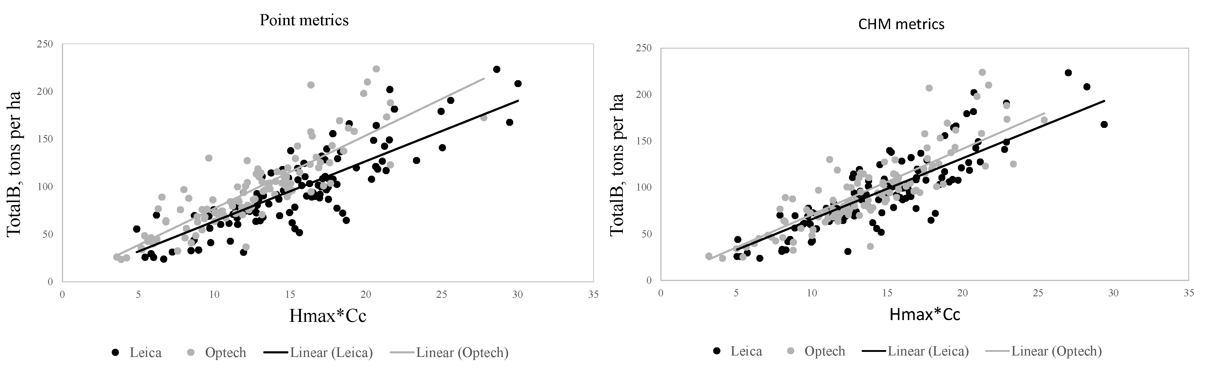
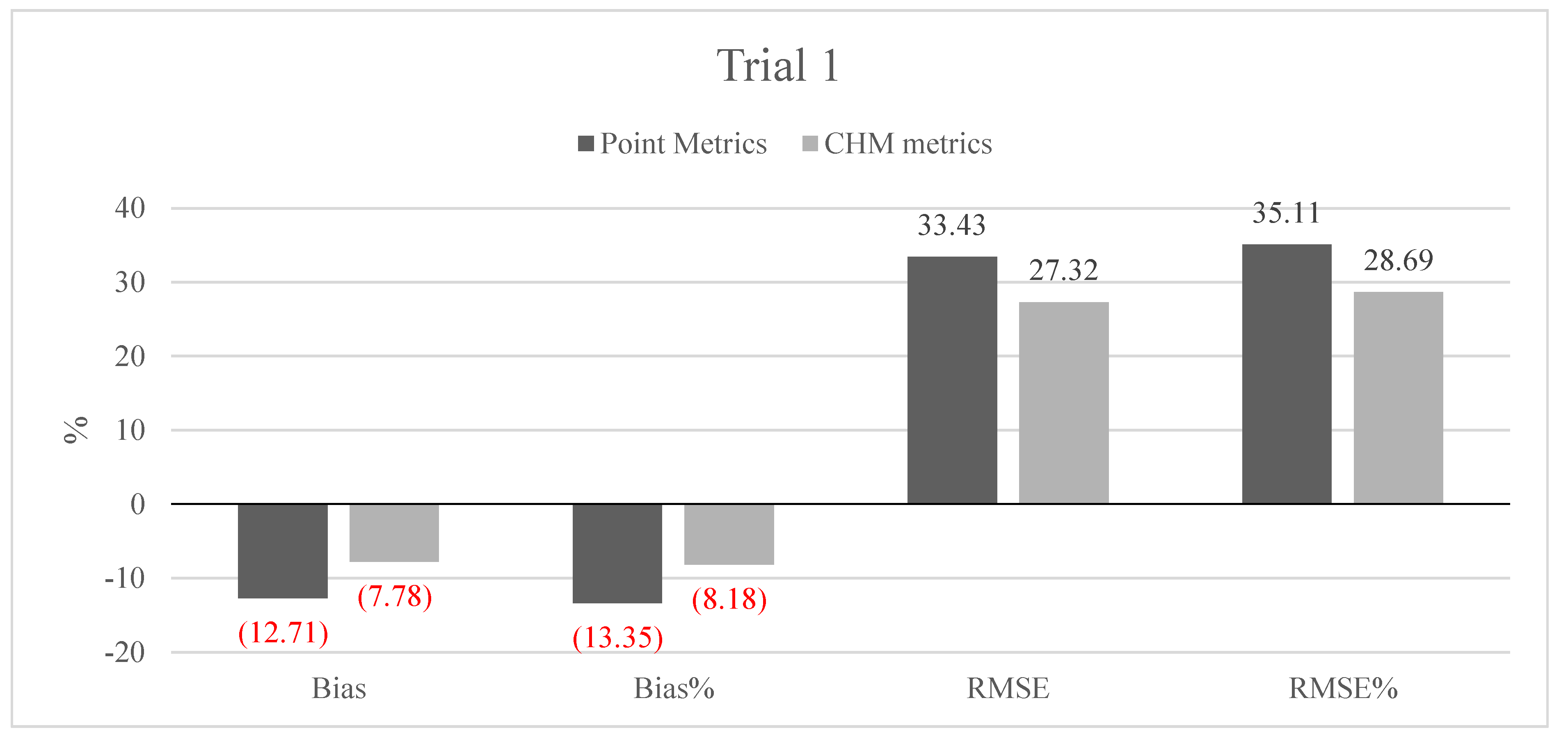
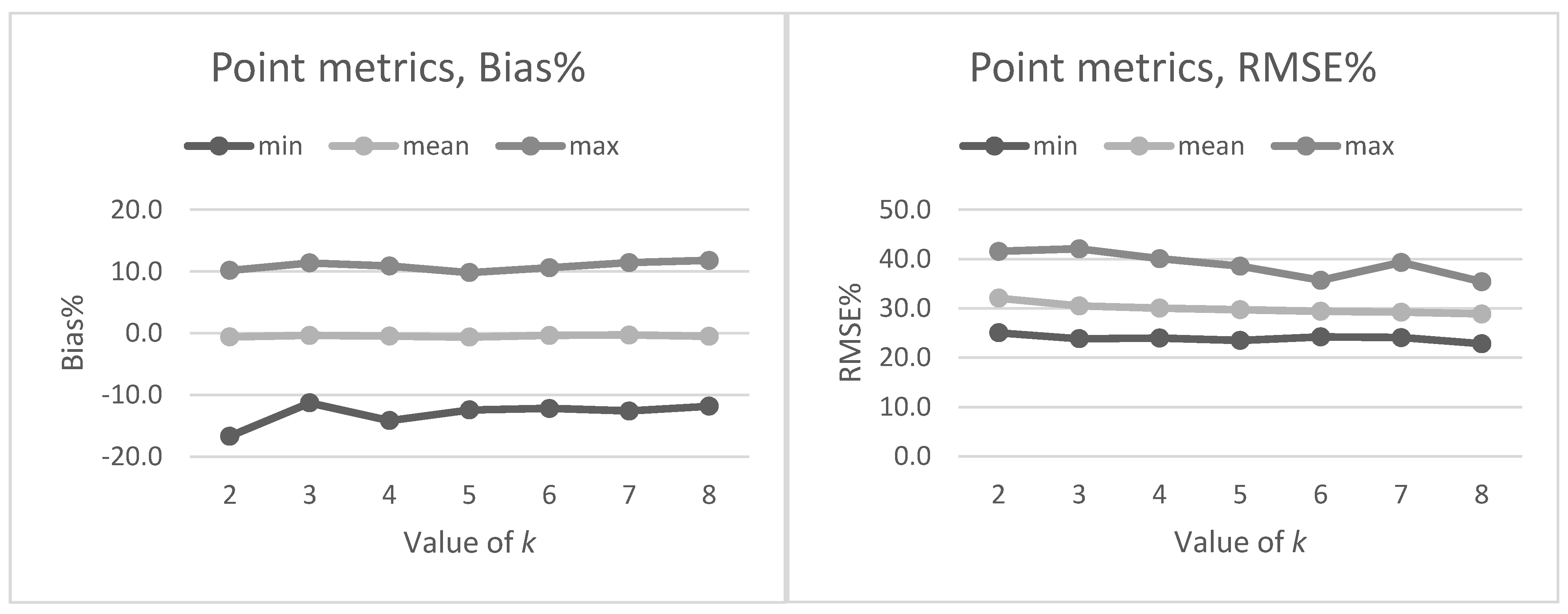
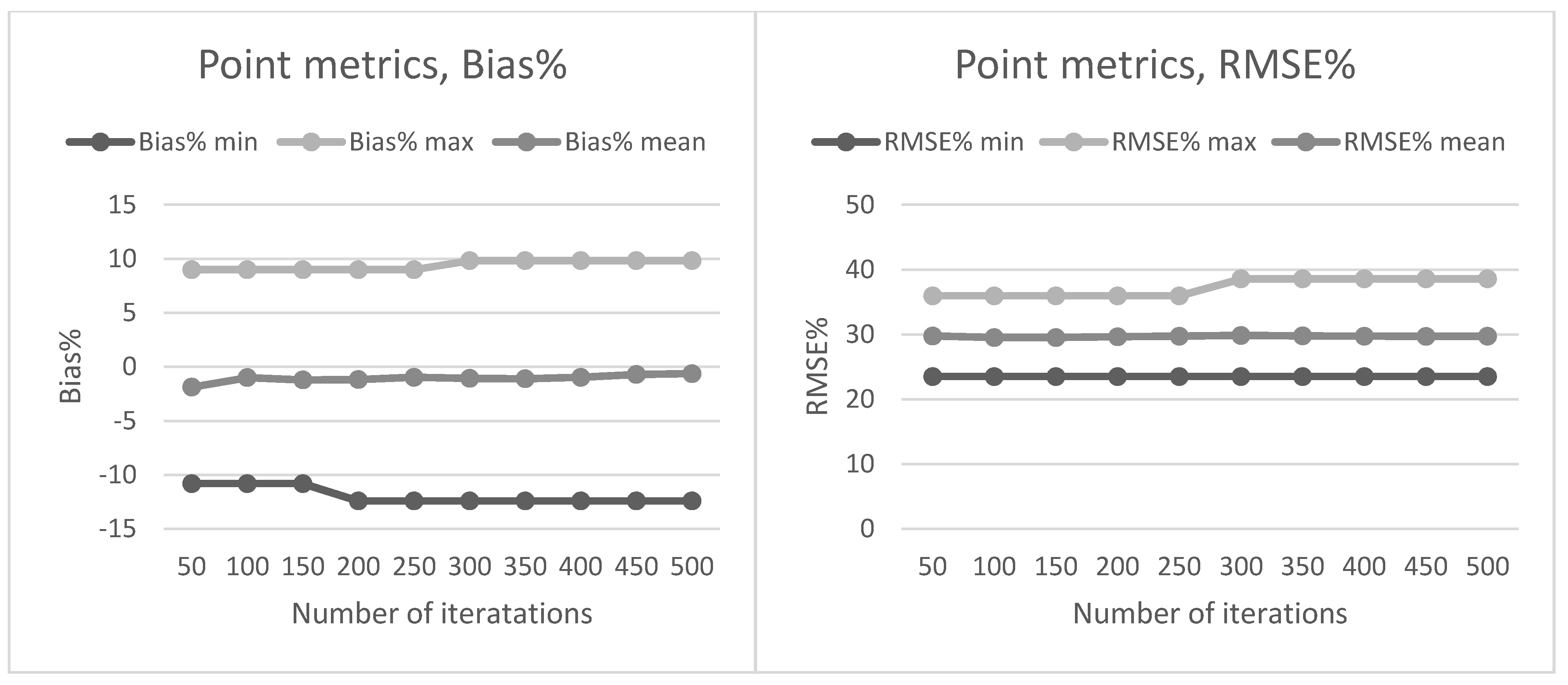
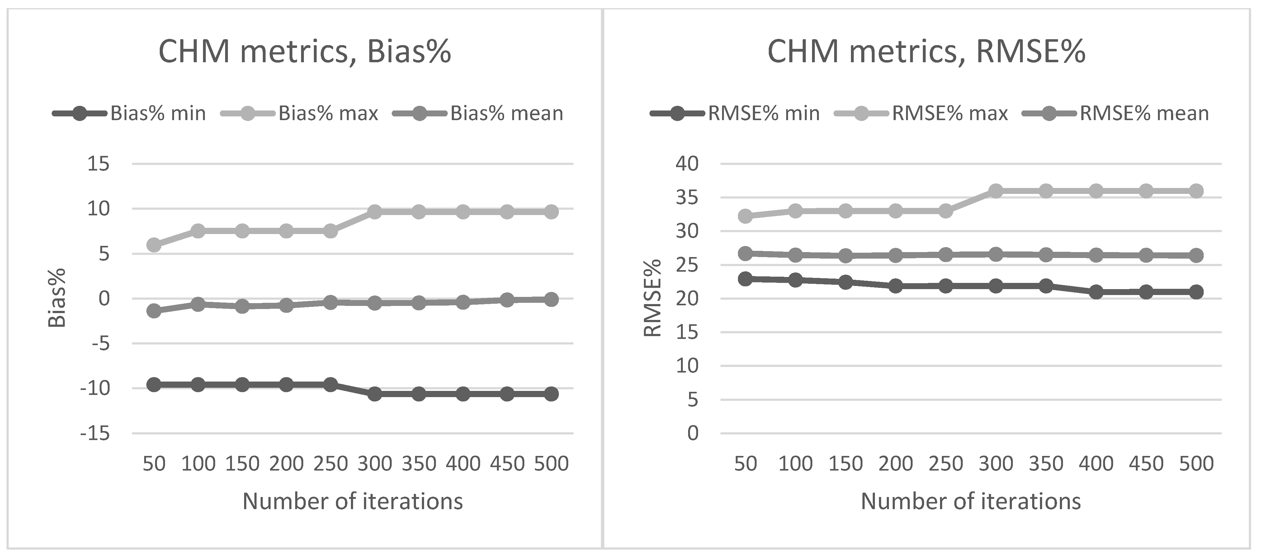
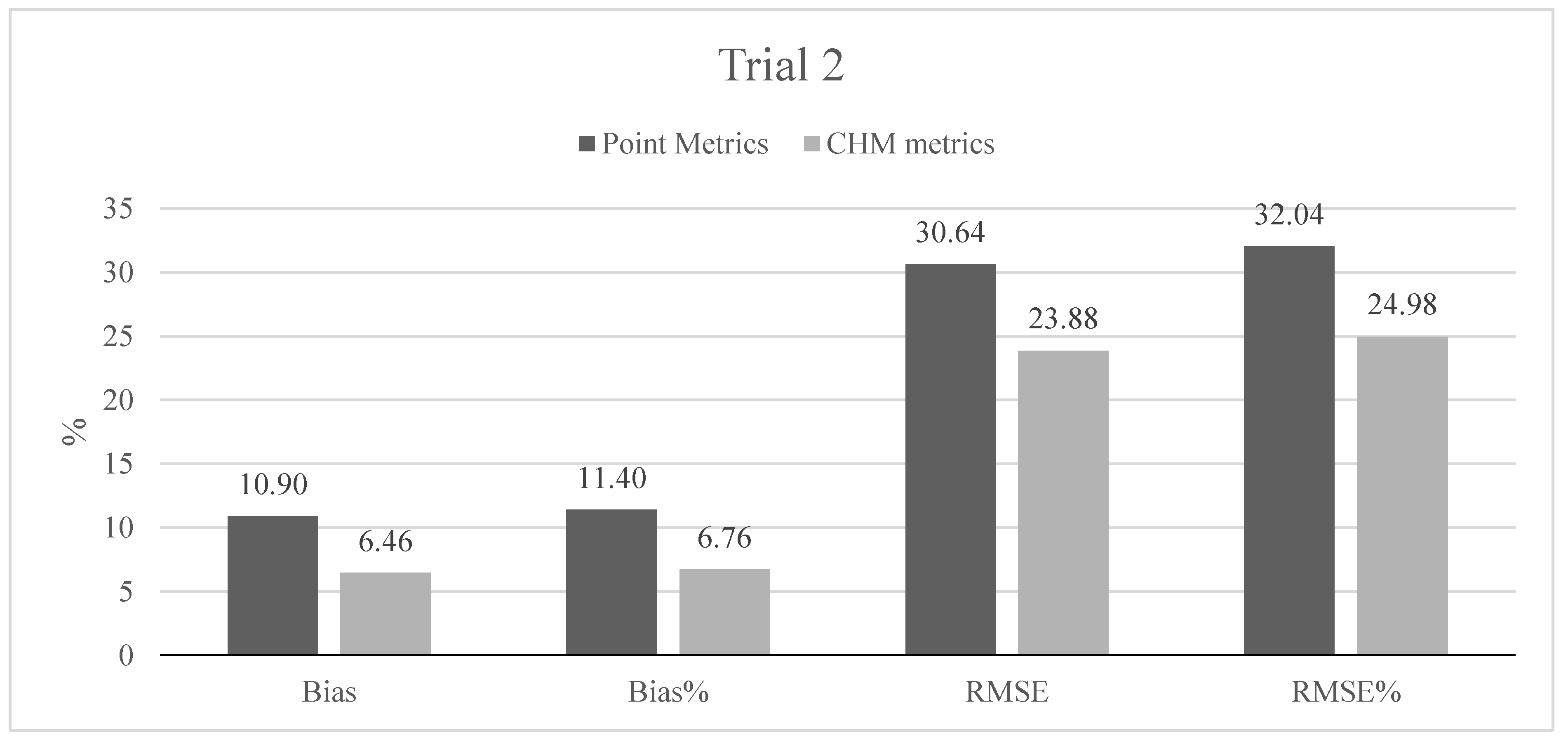
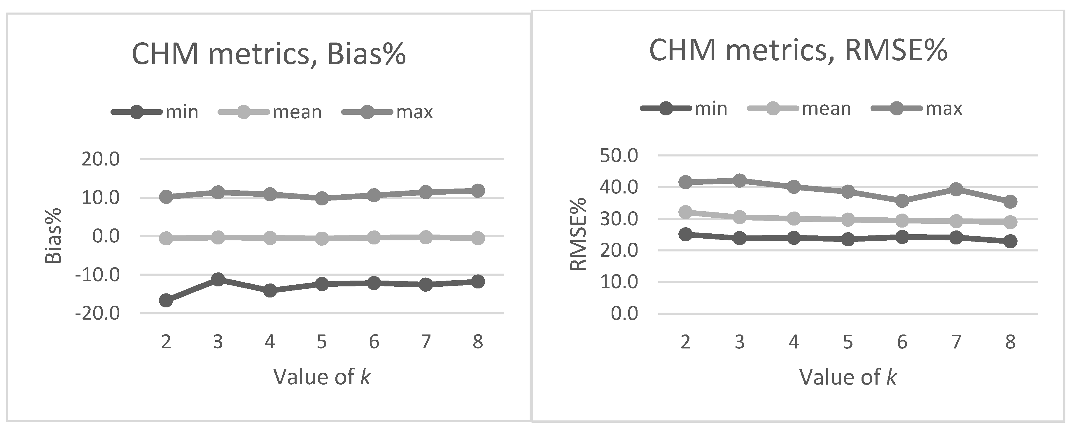
Section 2.2. The preliminary tests in our present study also showed that data acquisition parameters and sensors affected the metrics derived for predictions and thus the forest attribute predictions. The estimated bias caused by this effect was successfully reduced using the CHM-derived metrics as predictor variables in the NN predictions. The interpolation of the CHM simplifies the metrics used because it utilizes only the highest echo inside each pixel, but it still provides a detailed representation of the forest structure in terms of the variation of the top surface height. The effect was further evaluated by repeating the NN predictions 500 times to assess the model performance in detail. The CHM-derived metrics were slightly more stable and resulted in a smaller estimated bias but the difference was not as clear as in the first results. Therefore, this approach warrants further testing where all the external factors (such as data composition, area coverage and forest structure) are minimized.
The AGB components were predicted with similar accuracies to that reported previously (e.g., [17,24,25,
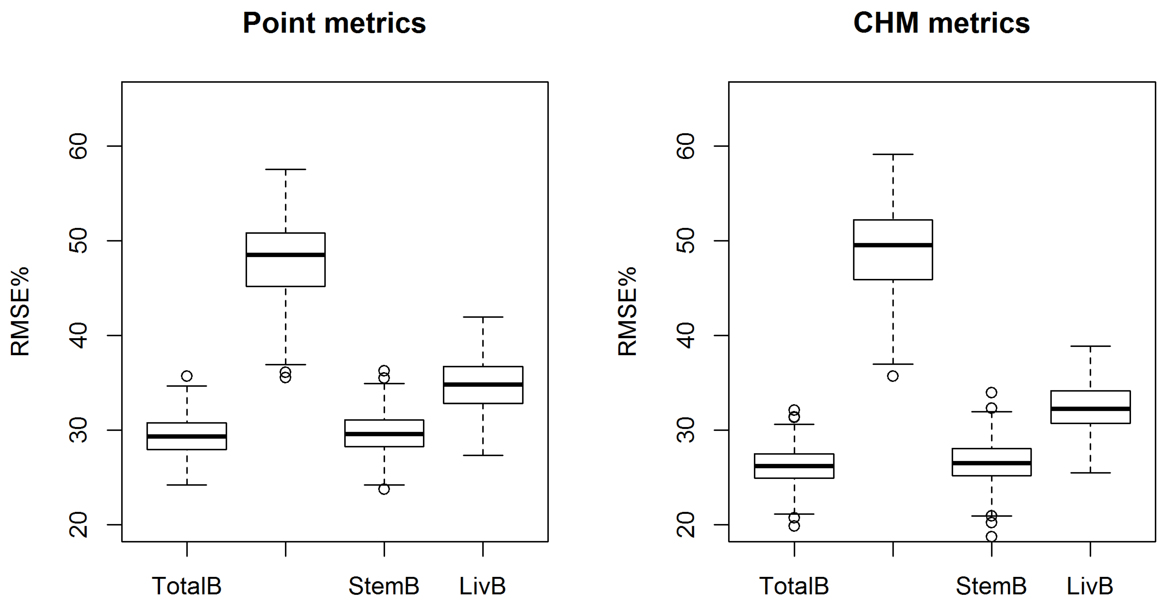
38]) using the NN approach with both metric data sets (point or CHM). The RMSE of totalB was 29.7% using ALS point metrics as predictor variables. The accuracy was further improved using CHM-derived metrics. The RMSE decreased to 26.4% and the minor negative estimated bias visible with the point metrics was reduced to near zero. Kankare et al. [24] used higher-density ALS data in the same study area (Evo), and achieved an RMSE of 24.9% for totalB. Latifi et al. [20] achieved plot-level accuracies of 22.2%–45.5% for totalB, using high-density ALS data. The best results were achieved with the RF approach in comparison to other NN methodologies [20]. Vastaranta et al. [39] compared ALS and high spatial resolution digital stereo imagery (DSI) in forest attribute prediction and achieved RMSE% of 17.5% and 23.7%, respectively. The results presented in our present study were achieved at a much lower pulse density (0.8 points per m2) than Kankare et al. [24], Latifi et al. [20] or Vastaranta et al. [39], which shows the potential of this data set in forest mapping applications. The use of the DSI-derived metrics provides another cost-efficient option for forest AGB mapping and monitoring [39]. However, to adequately compare the results and methods used, all external factors (e.g., site-specific or a selection of model features) should be removed.
The AGB component prediction accuracies were also improved using the CHM metrics. Only the RMSE of canopyB was increased (by 1.3%), but the decrease in the estimated bias was notable. The increase in the RMSE was most probably caused by the amount of dead branch biomass, which is shown to be a challenging attribute to predict [24]. He et al. [40] reported even higher accuracies for component biomass prediction using ALS data with similar densities. The ABA methods are also highly dependent on the training data available and in our study we were able to use 126 circular field-measured sample plots (~300 m2) in training. The increment of accuracy in He et al. [40] compared to our present study is most likely caused by the difference in sample plot size and the difference in forest structure and conditions. He et al. [40] used either 20 m × 20 m or 25 m × 25 m sample plots, an increase which tends to improve the prediction accuracies (e.g., [41,42]). Optimization of the amount and plot size of required training data for forest mapping with low density ALS data would be an important topic for future research.
The data acquisition period was not optimized for forest attribute prediction, and it is one important development steps for the method used here. The leaf-off period can especially affect the prediction accuracy of deciduous tree-dominated forests, but in our study area the deciduous trees are a minority and coniferous trees (Scots pine and Norway spruce) are the dominant tree species, comprising 78.2% of the total volume.
The sparse density, leaf-off ALS-data are an interesting possible alternative for cost-efficient forest mapping over larger areas. Nord-Larsen and Schumacher [29] and Villikka et al. [30] previously verified that this type of data collected for elevation modeling could also be suitable for forest attribute prediction, but did not compare the accuracy levels obtained with any existing technique such as MS-NFI. To be plausibly considered by the actors of operational forestry, a new forest-mapping method should have an accuracy comparable to that produced by existing inventory methods. The accuracies achieved in our study are higher, compared to those of the MS-NFI with the RMSE of totalB 47.7%, which was notably lower than the results based on the ALS data in our study. The difference in the prediction accuracy was caused by the prediction methods and the RS data used. MS-NFI utilizes satellite images and NFI-measured sample plots, resulting in 20 m × 20 m pixel-sized thematic maps on the forest attributes. The resolution of the RS data and the resampling procedure will have an effect on the prediction accuracies, which could potentially be minimized with higher resolution RS data. The data resolution used in our study was 1 m × 1 m for the DTM and CHM. The location accuracy (x, y) of the sample plots will have an effect on the prediction accuracies, but it is minimized during the field measurement campaigns by positioning the sample plot completely inside the forest stand. The location accuracy will have the most effect if the sample plot is located at the border of forest stand or in the middle of two stands.

5. Conclusions

Our study demonstrated that low-density, leaf-off ALS data originally collected for ground elevation modeling can be used for accurate component-level forest AGB prediction. Using metrics derived from the ALS point cloud, component-level prediction accuracies of 29.7%–48.3% can be achieved. The ALS data collected using varying scanning sensors and parameters was expected to have a notable effect on forest attribute prediction accuracies. Our study demonstrated a practical method for minimizing this effect using CHM-derived metrics in the predictions. This approach seemed to affect particularly the estimated bias, although the repeatability of these results warrants further evaluations. The prediction accuracies were also higher compared to the existing MS-NFI technique, which is widely used in practice. The prediction accuracy was higher mostly due to the RS data and prediction techniques used. To fully utilize the potential of ALS data in applications corresponding to this study, the following questions should be addressed: (1) the optimal amount of training data required for NN predictions and sample plots size; and (2) calibration of the ALS data caused by leaf-off situations.

Acknowledgments

Our study was made possible by financial aid from Metsämiesten säätiö, the Finnish Academy project Centre of Excellence in Laser Scanning Research (CoE-LaSR, decision number 272195) and the Finnish Academy project ‘Science and Technology Towards Precision Forestry’ (PreciseFor).

Author Contributions

Ville Kankare was the lead author in the present study. Jari Vauhkonen was responsible for metric extraction from the data sets. The article was improved by the contributions of the co-authors at various stages of the planning, data collection, analysis and writing process. We also want to acknowledge the anonymous reviewers who contributed constructive and important comments and suggestions to the article.

Appendix

A. Tuning the Value of k in NN Predictions

We investigated the effect of k-value on NN predictions by varying the k-value from 2 to 8. Results of these separate runs are shown in Table A1, Table A2 and Figure A1, Figure A2. RMSE% reduced 2.6% if the k-value of 6 was used compared to the k-value of 2 with CHM metrics. The difference between minimum and maximum values of RMSE% was also found to be smallest with the k-value of 6. Therefore the optimal k-value was set as 6 for the final calculations.
Table A1. The effect of k-value to the estimated bias% and RMSE% of totalB using point metrics as predictor variables.
k−value
2345678
BIAS%
min−16.7−11.3−14.1−12.4−12.2−12.6−11.8
mean−0.6−0.3−0.5−0.6−0.4−0.3−0.5
max10.211.410.99.810.611.411.8
RMSE%
min25.023.824.023.524.224.122.8
mean32.130.530.029.729.429.228.9
max41.642.140.138.635.739.335.4
Figure A1. The effect of k-value to the estimated bias% (right) and RMSE% (left) of totalB using point metrics as predictor variables.
Forests 06 01839 g004
Table A2. The effect of k-value to the estimated bias% and RMSE% of totalB using CHM metrics as predictor variables.
Value of k
2345678
BIAS%
min−10.8−10.7−10.7−10.6−9.7−13.5−11.3
mean0.10.10.0−0.10.20.1−0.1
max10.210.69.99.610.39.813.3
RMSE%
min23.120.821.721.019.920.620.2
mean28.827.526.826.426.225.925.7
max34.432.735.436.032.132.631.2
Figure A2. The effect of k-value to the estimated bias% (right) and RMSE% (left) of totalB using CHM metrics as predictor variables.
Forests 06 01839 g005

B. Tuning the Number of Iterations in NN Predictions

The number of iterations was set to 500 based on analyzing the estimated bias% and RMSE% of totalB with varying number of iterations from 50 to 500 with an interval of 50. Both minimum and maximum values stabilized with lower number of repetitions (e.g., 300 iterations if the estimated bias% of totalB was considered when CHM metrics were used as predictor variables) but the mean estimated bias% and RMSE% slightly decreased if more iterations were used. Therefore, the amount of iterations was set to 500. Results of the analyses are presented in Figure A3 and Figure A4.
Figure A3. The effect of the number of iterations to the estimated bias% and RMSE% of totalB when point metrics were used as predictor variables. The effect was analyzed by varying number of iterations from 50 to 500 with an interval of 50.
Forests 06 01839 g006
Figure A4. The effect of the number of iterations to estimated bias% and RMSE% of totalB when CHM metrics were used as predictor variables. The effect was analyzed by varying number of iterations from 50 to 500 with an interval of 50.
Forests 06 01839 g007

Conflicts of Interest

The authors declare no conflict of interest.

References

  1. Repola, J. Biomass Equations for Birch in Finland. Silva Fenn. 2008, 42, 605–624. [Google Scholar] [CrossRef]
  2. Repola, J. Biomass equations for Scots pine and Norway spruce in Finland. Silva Fenn. 2009, 43, 625–647. [Google Scholar] [CrossRef]
  3. Tomppo, E.; Olsson, H.; Ståhl, G.; Nilsson, M.; Hagner, O.; Katila, M. Combining national forest inventory field plots and remote sensing data for forest databases. Remote Sens. Environ. 2008, 112, 1982–1999. [Google Scholar] [CrossRef]
  4. Lu, D. The potential and challenge of remote sensing-based biomass estimation. Int. J. Remote Sens. 2006, 27, 1297–1328. [Google Scholar] [CrossRef]
  5. Tuominen, S.; Eerikäinen, K.; Schibalski, A.; Haakana, M.; Lehtonen, A. Mapping biomass variables with a multi-source forest inventory technique. Silva Fenn. 2010, 44, 109–117. [Google Scholar] [CrossRef]
  6. Næsset, E. Determination of mean tree height of forest stands using airborne laser scanner data. ISPRS J. Photogramm. Remote Sens. 1997, 52, 49–56. [Google Scholar] [CrossRef]
  7. White, J.C.; Wulder, M.A.; Varhola, A.; Vastaranta, M.; Coops, N.C.; Cook, B.D.; Pitt, D.; Woods, M. A best practices guide for generating forest inventory attributes from airborne laser scanning data using an area-based approach. For. Chron. 2013, 89, 722–723. [Google Scholar] [CrossRef]
  8. Hyyppä, J.; Inkinen, M. Detecting and estimating attributes for single trees using laser scanner. Photogramm. J. Finl. 1999, 16, 27–42. [Google Scholar]
  9. Hauglin, M.; Gobakken, T.; Astrup, R.; Ene, L.; Næsset, E. Estimating Single-Tree Crown Biomass of Norway Spruce by Airborne Laser Scanning: A Comparison of Methods with and without the Use of Terrestrial Laser Scanning to Obtain the Ground Reference Data. Forests 2014, 5, 384–403. [Google Scholar] [CrossRef]
  10. Kankare, V.; Holopainen, M.; Vastaranta, M.; Puttonen, E.; Yu, X.; Hyyppä, J. Individual tree biomass estimation using terrestrial laser scanning. ISPRS J. Photogramm. Remote Sens. 2013, 75, 64–75. [Google Scholar] [CrossRef]
  11. Kankare, V.; Räty, M.; Yu, X.; Holopainen, M.; Vastaranta, M.; Kantola, T.; Hyyppä, J.; Hyyppä, H.; Alho, P.; Viitala, R. Single tree biomass modelling using airborne laser scanning. ISPRS J. Photogramm. Remote Sens. 2013, 85, 66–73. [Google Scholar] [CrossRef]
  12. Popescu, S.C. Estimating biomass of individual pine trees using airborne lidar. Biomass Bioenergy 2007, 31, 646–655. [Google Scholar] [CrossRef]
  13. Hauglin, M.; Dibdiakova, J.; Gobakken, T.; Næsset, E. Estimating single-tree branch biomass of Norway spruce by airborne laser scanning. ISPRS J. Photogramm. Remote Sens. 2013, 79, 147–156. [Google Scholar] [CrossRef]
  14. Hauglin, M.; Astrup, R.; Gobakken, T.; Næsset, E. Estimating single-tree branch biomass of Norway spruce with terrestrial laser scanning using voxel-based and crown dimension features. Scand. J. For. Res. 2013, 28, 456–469. [Google Scholar] [CrossRef]
  15. Zolkos, S.G.; Goetz, S.J.; Dubayah, R. A meta-analysis of terrestrial aboveground biomass estimation using lidar remote sensing. Remote Sens. Environ. 2013, 128, 289–298. [Google Scholar] [CrossRef]
  16. Popescu, S.C.; Hauglin, M. Estimation of biomass components by airborne laser scanning. In Forestry Applications of Airborne Laser Scanning—Concepts and Case Studies; Maltamo, M., Næsset, E., Vauhkonen, J., Eds.; Managing Forest Ecosystems 27; Springer: Dordrecht, The Netherlands, 2014; pp. 157–175. [Google Scholar]
  17. Popescu, S.C.; Wynne, R.H.; Scrivani, J.A. Fusion of Small-Footprint Lidar and Multispectral Data to Estimate Plot- Level Volume and Biomass in Deciduous. For. Sci. 2004, 50, 551–565. [Google Scholar]
  18. Aardt, J.A.N.; van Wynne, R.H.; Oderwald, R.G. Lidar-Distributional Parameters on a Per-Segment Basis. For. Sci. 2006, 52, 636–649. [Google Scholar]
  19. Næsset, E. Practical Large-Scale Forest Stand Inventory Using a Small-Footprint Airborne Scanning Laser. Scand. J. For. Res. 2004, 19, 164–179. [Google Scholar] [CrossRef]
  20. Latifi, H.; Nothdurft, A.; Koch, B. Non-parametric prediction and mapping of standing timber volume and biomass in a temperate forest: Application of multiple optical/LiDAR-derived predictors. Forestry 2010, 83, 395–407. [Google Scholar] [CrossRef]
  21. Fassnacht, F.E.; Hartig, F.; Lati, H.; Berger, C.; Hernández, J.; Corvalán, P.; Koch, B. Importance of sample size, data type and prediction method for remote sensing-based estimations of aboveground forest biomass. Remote Sens. Environ. 2014, 154, 102–114. [Google Scholar] [CrossRef]
  22. Stepper, C.; Straub, C.; Pretzsch, H. Using semi-global matching point clouds to estimate growing stock at the plot and stand levels : Application for a broadleaf-dominated forest in central Europe. Can. J. For. Res. 2015, 123, 111–123. [Google Scholar] [CrossRef]
  23. Vastaranta, M.; Kankare, V.; Holopainen, M.; Yu, X.; Hyyppä, J.; Hyyppä, H. Combination of individual tree detection and area-based approach in imputation of forest variables using airborne laser data. ISPRS J. Photogramm. Remote Sens. 2012, 67, 73–79. [Google Scholar] [CrossRef]
  24. Kankare, V.; Vastaranta, M.; Holopainen, M.; Räty, M.; Yu, X.; Hyyppä, J.; Hyyppä, H.; Alho, P.; Viitala, R. Retrieval of forest aboveground biomass and stem volume with airborne scanning LiDAR. Remote Sens. 2013, 5, 2257–2274. [Google Scholar] [CrossRef] [Green Version]
  25. Tuominen, S.; Haapanen, R. Estimation of forest biomass by means of genetic algorithm-based optimization of airborne laser scanning and digital aerial photograph features. Silva Fenn. 2013, 47, 20. [Google Scholar] [CrossRef]
  26. Bohlin, J.; Wallerman, J.; Fransson, J.E.S. Forest variable estimation using photogrammetric matching of digital aerial images in combination with a high-resolution DEM. Scand. J. For. Res. 2012, 27, 692–699. [Google Scholar] [CrossRef]
  27. Dalponte, M.; Martinez, C.; Rodeghiero, M.; Gianelle, D. The role of ground reference data collection in the prediction of stem volume with LiDAR data in mountain areas. ISPRS J. Photogramm. Remote Sens. 2011, 66, 787–797. [Google Scholar] [CrossRef]
  28. Gomez-Gutierrez, A.; Schnabel, S.; Lavado-Contador, F.; Garcia-Marin, R. Testing the quality of open-access DEMs and their derived attributes in Spain : SRTM, GDEM and PNOA DEM. In Proceedings of Geomorphometry 2011 Conference, Redlands, CA, USA, 2011; pp. 53–56.
  29. Nord-Larsen, T.; Schumacher, J. Estimation of forest resources from a country wide laser scanning survey and national forest inventory data. Remote Sens. Environ. 2012, 119, 148–157. [Google Scholar] [CrossRef]
  30. Villikka, M.; Packalén, P.; Maltamo, M. The Suitability of Leaf-off Airborne Laser Scanning Data in an Area-based Forest Inventory of Coniferous and Deciduous Trees. Silva Fenn. 2012, 46, 99–110. [Google Scholar] [CrossRef]
  31. Næsset, E. Predicting forest stand characteristics with airborne scanning laser using a practical two-stage procedure and field data. Remote Sens. Environ. 2002, 80, 88–99. [Google Scholar] [CrossRef]
  32. Korhonen, L.; Peuhkurinen, J.; Malinen, J.; Suvanto, A.; Maltamo, M.; Packalén, P.; Kangas, J. The use of airborne laser scanning to estimate sawlog volumes. Forestry 2008, 81, 499–510. [Google Scholar]
  33. Hudak, A.T.; Crookston, N.L.; Evans, J.S.; Hall, D.E.; Falkowski, M.J. Nearest neighbor imputation of species-level, plot-scale forest structure attributes from LiDAR data. Remote Sens. Environ. 2008, 112, 2232–2245. [Google Scholar] [CrossRef]
  34. Crookston, N.L.; Finley, A.O. yaImpute: An R package for kNN imputation. J. Stat. Softw. 2008, 23, 1–16. [Google Scholar]
  35. R Core Team. R: A language and environment for statistical computing. Avaliable online: http://www.r-project.org/ (accessed on 12 January 2014).
  36. Tomppo, E.; Halme, M. Using coarse scale forest variables as ancillary information and weighting of variables in k-NN estimation: A genetic algorithm approach. Remote Sens. Environ. 2004, 92, 1–20. [Google Scholar] [CrossRef]
  37. Næsset, E. Effects of different sensors, flying altitudes, and pulse repetition frequencies on forest canopy metrics and biophysical stand properties derived from small-footprint airborne laser data. Remote Sens. Environ. 2009, 113, 148–159. [Google Scholar] [CrossRef]
  38. Kotamaa, E.; Tokola, T.; Maltamo, M.; Packalén, P.; Kurttila, M.; Mäkinen, A. Integration of remote sensing-based bioenergy inventory data and optimal bucking for stand-level decision making. Eur. J. For. Res. 2010, 129, 875–886. [Google Scholar] [CrossRef]
  39. Vastaranta, M.; Wulder, M.A.; White, J.C.; Pekkarinen, A.; Tuominen, S.; Ginzler, C.; Kankare, V.; Holopainen, M.; Hyyppa, J.; Hyyppa, H. Airborne laser scanning and digital stereo imagery measures of forest structure : Comparative results and implications to forest mapping and inventory update. Can. J. Remote Sens. 2013, 39, 382–395. [Google Scholar] [CrossRef]
  40. He, Q.; Chen, E.; An, R.; Li, Y. Above-Ground Biomass and Biomass Components Estimation Using LiDAR Data in a Coniferous Forest. Forests 2013, 4, 984–1002. [Google Scholar] [CrossRef]
  41. Næsset, E.; Gobakken, T. Estimation of above- and below-ground biomass across regions of the boreal forest zone using airborne laser. Remote Sens. Environ. 2008, 112, 3079–3090. [Google Scholar] [CrossRef]
  42. Næsset, E.; Gobakken, T.; Bollandsås, O.M.; Gregoire, T.G.; Nelson, R.; Ståhl, G. Comparison of precision of biomass estimates in regional field sample surveys and airborne LiDAR-assisted surveys in Hedmark County, Norway. Remote Sens. Environ. 2013, 130, 108–120. [Google Scholar] [CrossRef]

