
Commercial Thinning to Meet Wood Production Objectives and Develop Structural Heterogeneity: A Case Study in the Spruce-Fir Forest, Quebec, Canada


Abstract
:1. Introduction
2. Experimental Section
2.1. Study Site

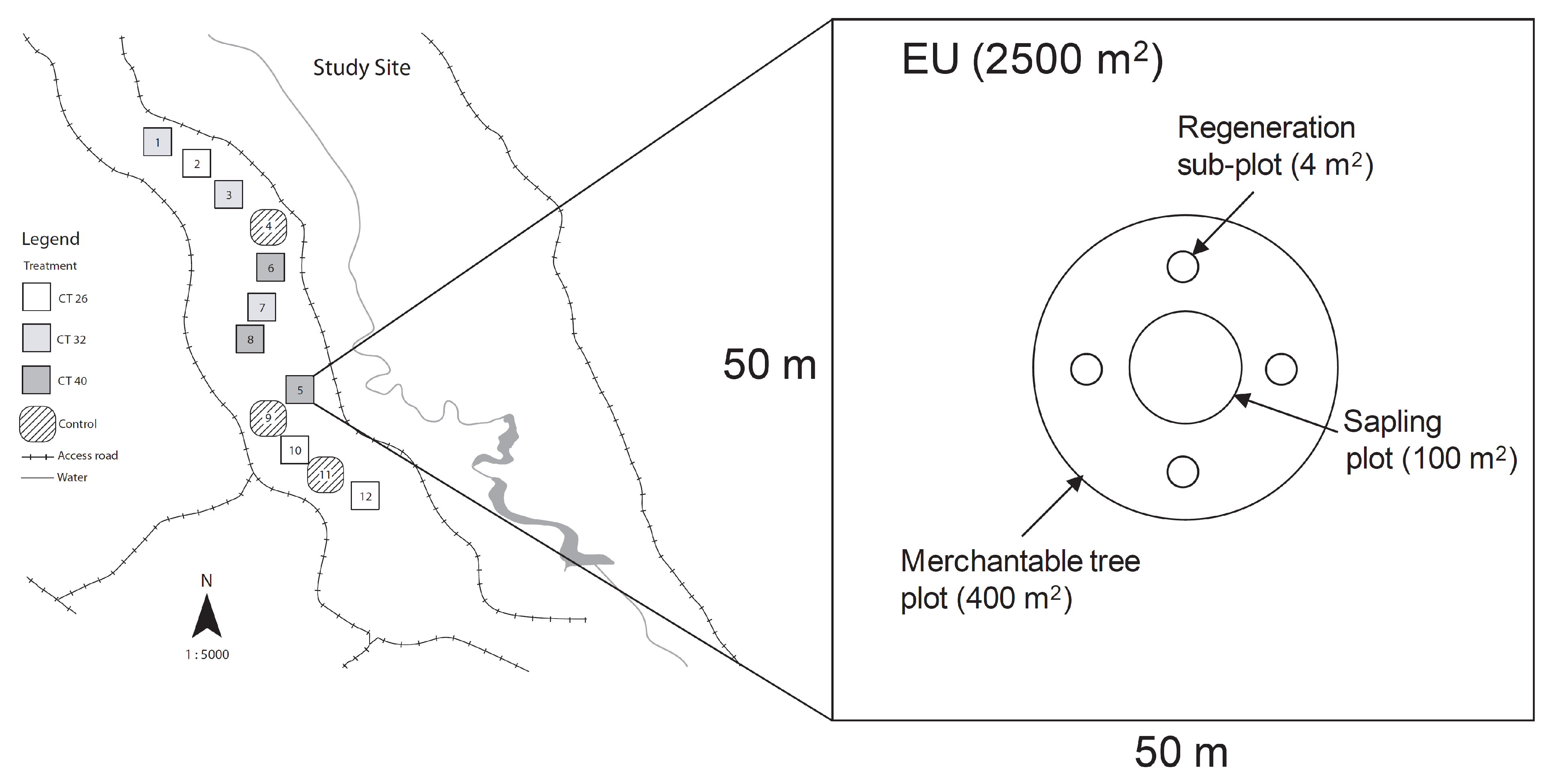
| Thinning | Characteristic | Preharvest | Postharvest | ||
|---|---|---|---|---|---|
| Treatment | Mean | SE | Mean | SE | |
| CT26 | Age (y) | –– | –– | 54 | 8 |
| SI (m) | –– | –– | 14 | 0.4 | |
| DBHq (cm) | 16.1 | 0.5 | 16.9 | 0.5 | |
| Ht (m) | 12.3 | 0.4 | 12.1 | 0.5 | |
| Density (trees ha–1) | 1667 | 209 | 1108 | 110 | |
| RD | 0.56 | 0.06 | 0.41 | 0.04 | |
| BA (m2 ha–1) | 33.6 | 3.5 | 24.9 | 2.2 | |
| GMV (m3 ha–1) | 186 | 22 | 136 | 14 | |
| Slenderness ratio | 0.80 | 0.03 | 0.74 | 0.03 | |
| Live crown ratio | –– | –– | 0.55 | 0.08 | |
| CT32 | Age (y) | –– | –– | 58 | 4 |
| SI (m) | –– | –– | 14 | 0.1 | |
| DBHq (cm) | 16.3 | 0.4 | 17.8 | 0.5 | |
| Height (m) | 12.4 | 0.2 | 12.5 | 0.1 | |
| Density (trees ha–1) | 1517 | 228 | 867 | 145 | |
| RD | 0.53 | 0.07 | 0.36 | 0.05 | |
| BA (m2 ha–1) | 31.4 | 3.3 | 21.3 | 2.6 | |
| GMV (m3 ha–1) | 174 | 18 | 119 | 14 | |
| Slenderness ratio | 0.79 | 0.02 | 0.72 | 0.02 | |
| Live crown ratio | –– | –– | 0.72 | 0.04 | |
| CT40 | Age (y) | –– | –– | 48 | 4 |
| SI (m) | –– | –– | 14 | 0.3 | |
| DBHq (cm) | 14.7 | 0.3 | 16.7 | 0.4 | |
| Height (m) | 11.3 | 0.2 | 11.7 | 0.4 | |
| Density (trees ha–1) | 1733 | 242 | 817 | 85 | |
| RD | 0.49 | 0.04 | 0.30 | 0.02 | |
| BA (m2 ha–1) | 29.5 | 2.2 | 17.8 | 1.5 | |
| GMV (m3 ha–1) | 145 | 13 | 93 | 9 | |
| Slenderness ratio | 0.79 | 0.01 | 0.72 | 0.01 | |
| Live crown ratio | –– | –– | 0.75 | 0.05 | |
| Control | Age (y) | –– | –– | 57 | 8 |
| SI (m) | –– | –– | 13 | 1.1 | |
| DBHq (cm) | 15.2 | 0.7 | 15.5 | 0.8 | |
| Height (m) | 11.7 | 0.5 | 12.0 | 0.6 | |
| Density (trees ha–1) | 1650 | 66 | 1625 | 76 | |
| RD | 0.49 | 0.04 | 0.50 | 0.05 | |
| Control | BA (m2 ha–1) | 30.1 | 1.9 | 30.5 | 2.4 |
| GMV (m3 ha–1) | 153 | 20 | 162 | 23 | |
| Slenderness ratio | 0.80 | 0.01 | 0.80 | 0.01 | |
| Live crown ratio | –– | –– | 0.79 | 0.03 |
2.2. Experimental Design and Thinning Treatments

2.3. Growth and Yield Measurements
2.4. Structural Heterogeneity Measurements
2.5. Statistical Analyses of Growth and Yield
2.6. Statistical Analyses of Structural Heterogeneity

3. Results
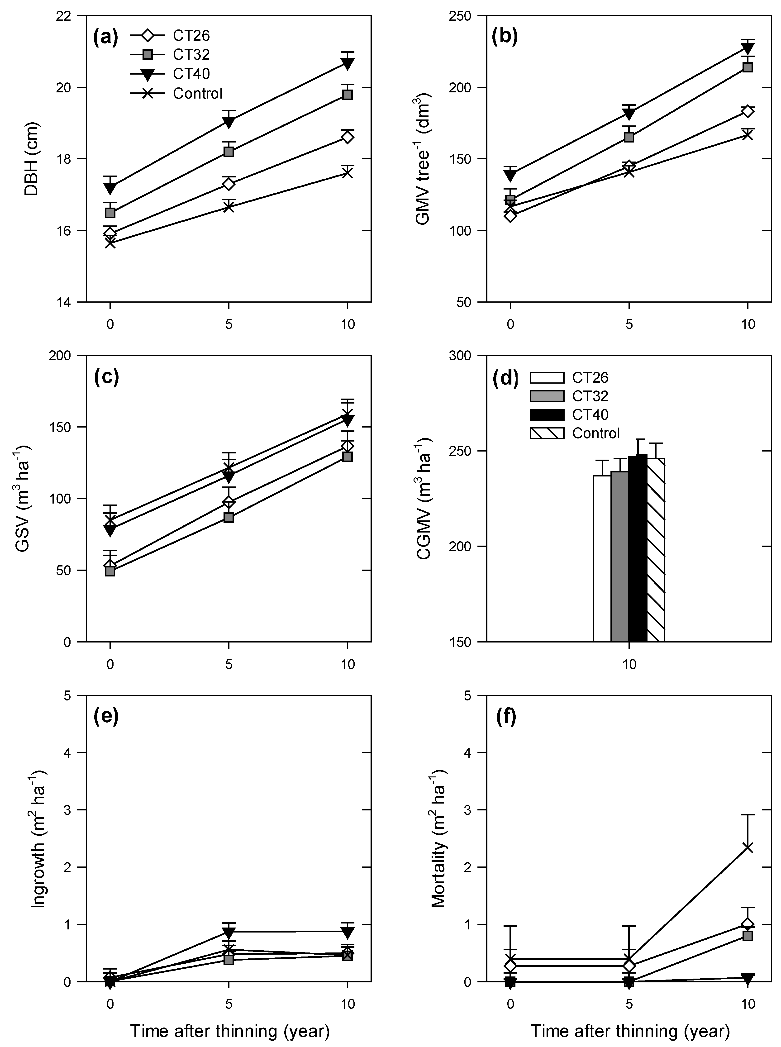
3.1. Growth and Yield
3.1.1. Mean Tree Level
| Objective | Response Variable | Source of Variation | ndf | ddf | F-Value | p-Value |
|---|---|---|---|---|---|---|
| Mean Tree | DBH | Thinning (T) | 3 | 5.9 | 19.7 | 0.002 |
| Level | (cm) | Year (Y) | 2 | 8.4 | 1345.0 | <0.001 |
| T × Y | 6 | 4.9 | 43.1 | <0.001 | ||
| Covariate (C) | 1 | 5.6 | 62.7 | <0.001 | ||
| GMV | T | 3 | 15.7 | 19.5 | <0.001 | |
| (dm3 tree–1) | Y | 2 | 11.6 | 724.6 | <0.001 | |
| T × Y | 6 | 8.4 | 10.6 | 0.002 | ||
| C | 1 | 1.6 | 120.6 | 0.018 | ||
| Stand Yield | GSV | T | 3 | 6.8 | 1.98 | 0.209 |
| (m3 ha–1) | Y | 2 | 15.2 | 131.46 | <0.001 | |
| T × Y | 6 | 15.2 | 0.17 | 0.982 | ||
| C | 1 | 6.7 | 31.65 | <0.001 | ||
| CGMV | T | 3 | 7.0 | 0.35 | 0.791 | |
| (m3 ha–1) | C | 1 | 7.0 | 79.42 | <0.001 | |
| Ingrowth | T | 3 | 10.2 | 2.03 | 0.172 | |
| (m2 ha–1) | Y | 2 | 17.5 | 19.81 | <0.001 | |
| T × Y | 6 | 17.5 | 0.95 | 0.489 | ||
| C | 1 | 10.3 | 7.23 | 0.022 | ||
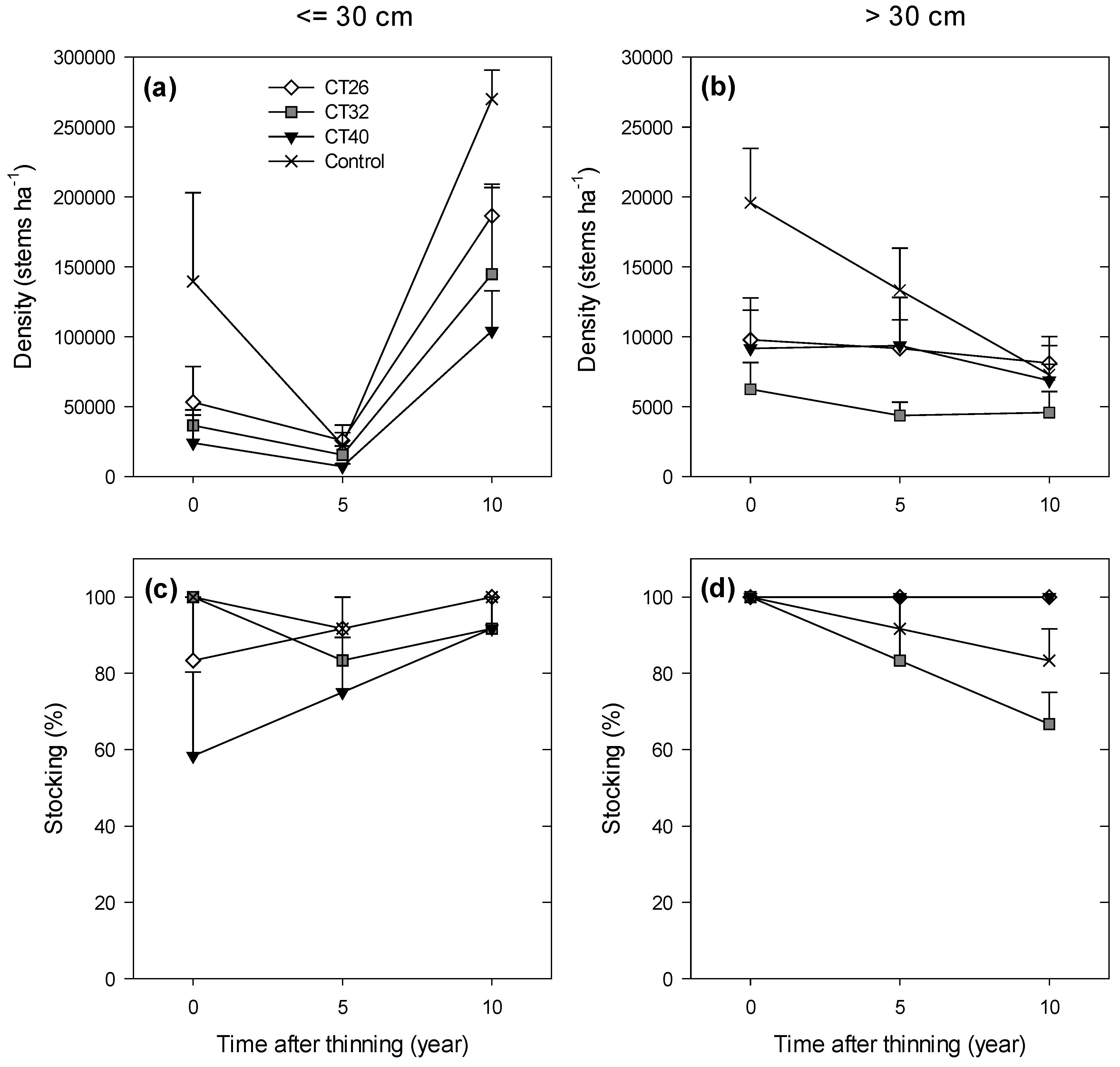
| Old-Growth | Density ≤ 30 cm | T | 3 | 8.0 | 1.43 | 0.303 |
| Attributes | (stems ha–1) | Y | 2 | 15.3 | 49.65 | <0.001 |
| (Regeneration) | T × Y | 6 | 15.3 | 1.14 | 0.386 | |
| Density > 30 cm | T | 3 | 8.0 | 1.80 | 0.226 | |
| (stems ha–1) | Y | 2 | 10.5 | 11.83 | 0.002 | |
| T × Y | 6 | 10.5 | 2.89 | 0.064 | ||
| Stocking ≤ 30 cm | T | 3 | 7.7 | 1.11 | 0.403 | |
| (%) | Y | 2 | 11.4 | 1.55 | 0.254 | |
| T × Y | 6 | 11.4 | 0.86 | 0.548 |
3.1.2. Stand Level

3.2. Structural Heterogeneity
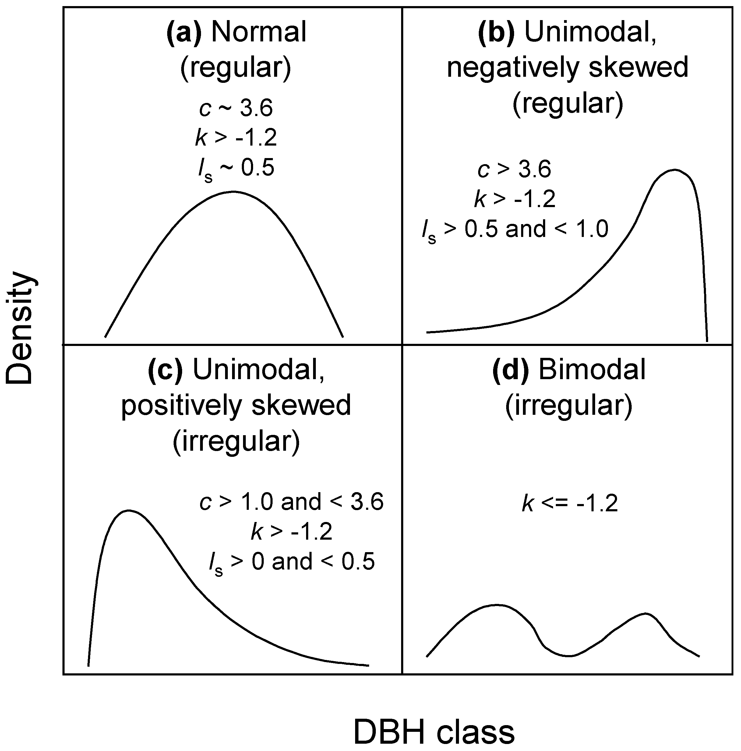
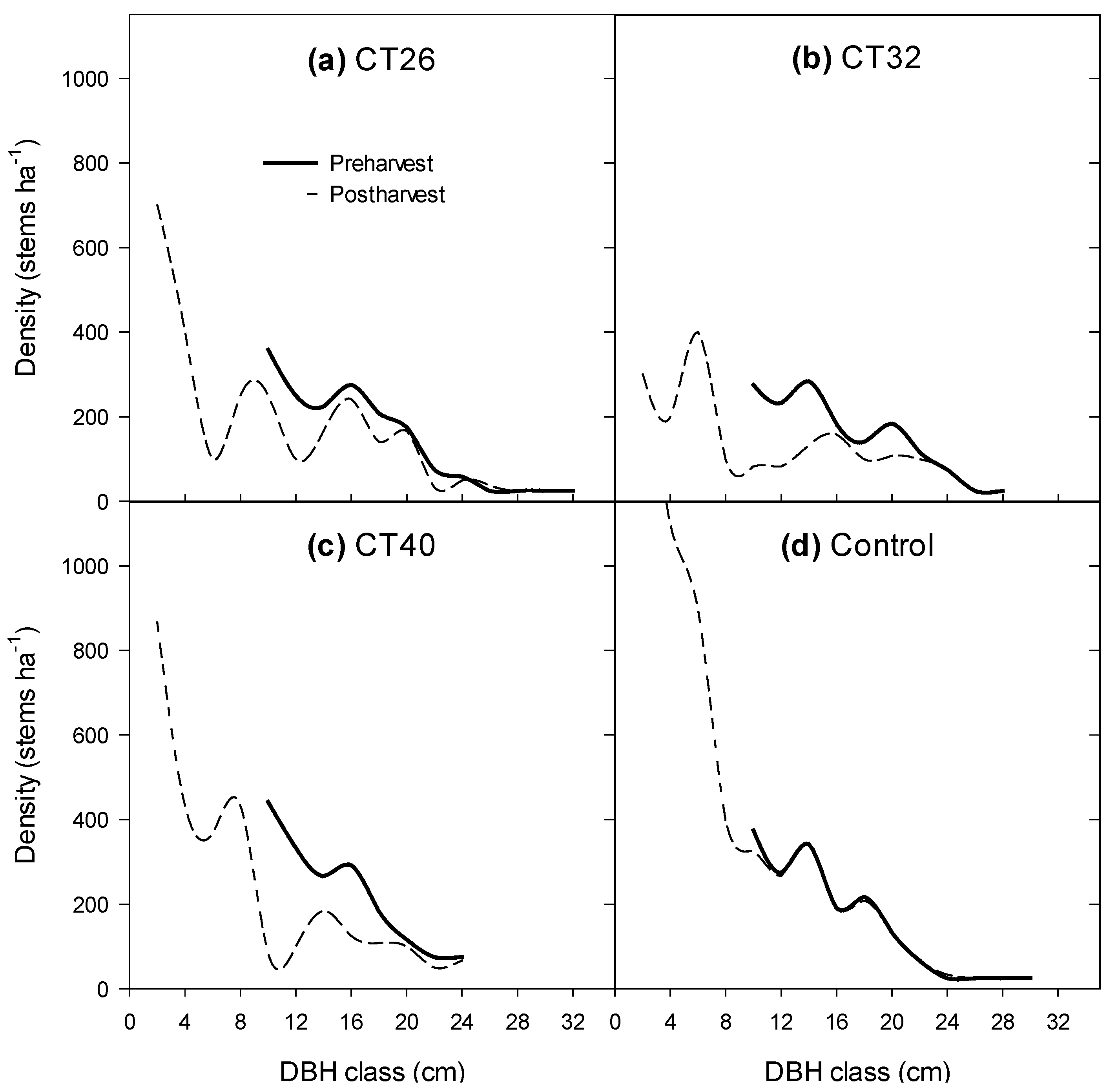
3.2.1. Number of Large Trees and Shape of the Diameter Distribution

| Trt | EU | c | K | Is | Structure | ||||
|---|---|---|---|---|---|---|---|---|---|
| Post | 10 y | Post | 10 y | Post | 10 y | Post | 10 y | ||
| CT26 | 2 | 3.8 | 5.4 | 0.4 | 0.1 | 0.65 | 0.68 | Regular | Regular |
| 10 | 1.1 | 1.0 | −0.6 | 1.0 | 0.05 | 0.04 | Irregular | Irregular | |
| 12 | 1.7 | 1.1 | 0.5 | −0.4 | 0.14 | 0.04 | Irregular | Irregular | |
| CT32 | 1 | 1.8 | 1.9 | −1.0 | −1.2 | 0.22 | 0.20 | Irregular | Irregular, bim |
| 3 | 1.2 | 1.5 | −1.3 | −1.4 | 0.04 | 0.04 | Irregular, bim | Irregular, bim | |
| 7 | 1.7 | 1.1 | −0.9 | −0.8 | 0.24 | 0.04 | Irregular | Irregular | |
| CT40 | 5 | 1.2 | 1.1 | 1.5 | 0.1 | 0.05 | 0.04 | Irregular | Irregular |
| 6 | 1.7 | 1.6 | −0.2 | −0.8 | 0.37 | 0.04 | Irregular | Irregular | |
| 8 | 1.4 | 1.5 | −0.3 | −0.9 | 0.05 | 0.04 | Irregular | Irregular | |
| Control | 4 | 1.1 | 1.0 | −1.1 | −1.1 | 0.05 | 0.04 | Irregular | Irregular |
| 9 | 1.5 | 1.6 | 0.3 | −1.1 | 0.06 | 0.14 | Irregular | Irregular | |
| 11 | 1.3 | 2.3 | −0.7 | −0.6 | 0.06 | 0.43 | Irregular | Irregular | |
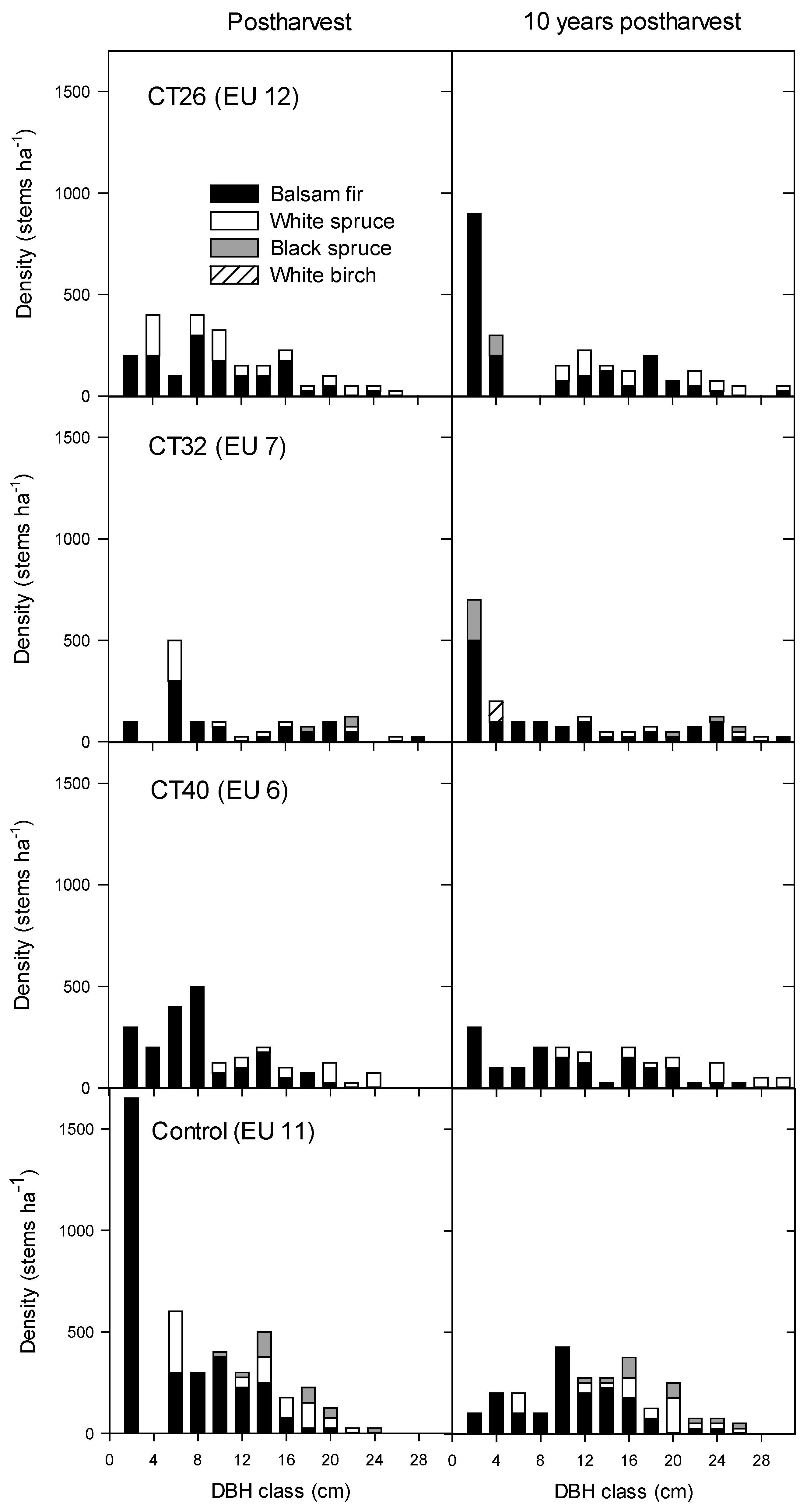
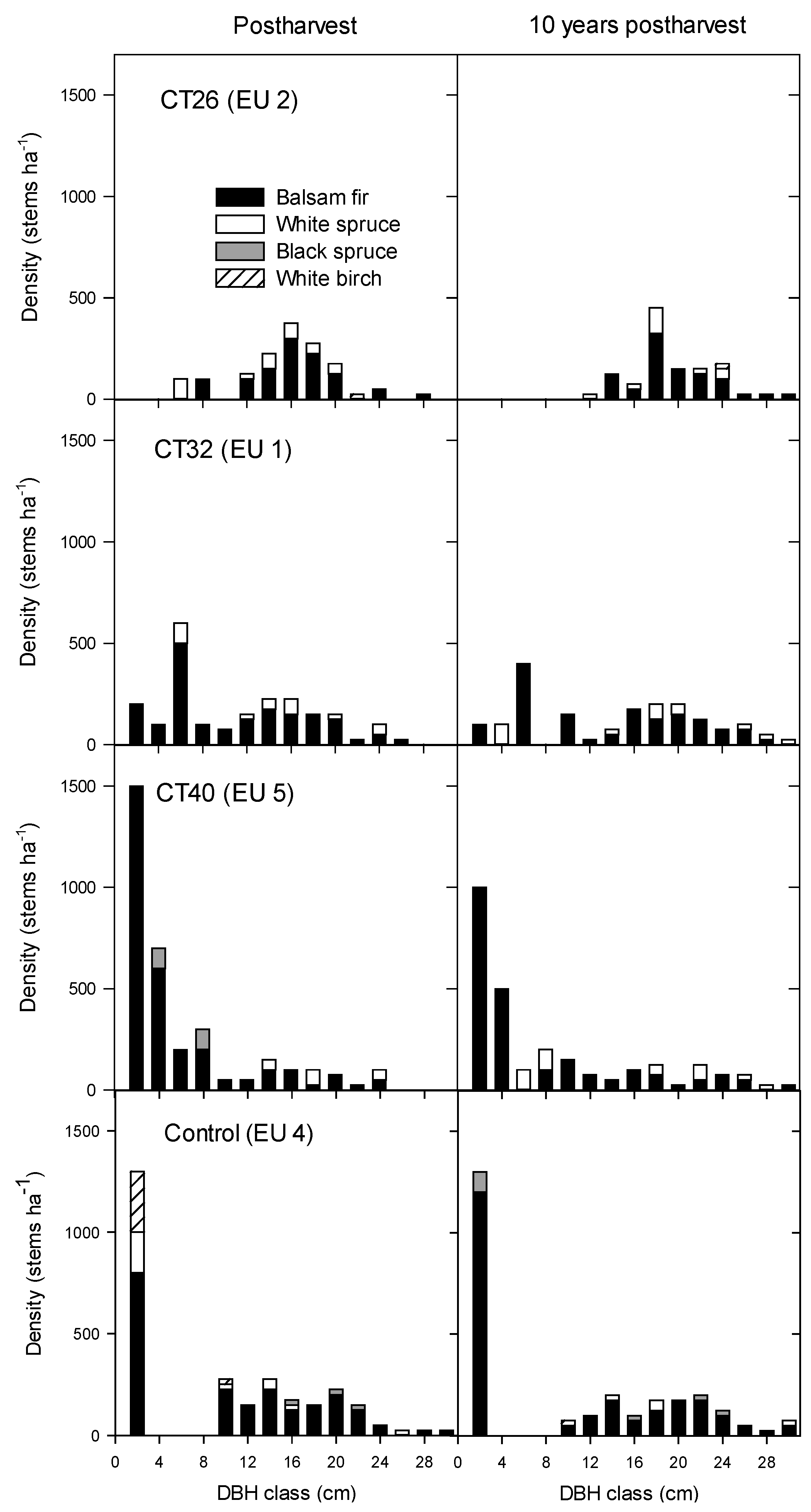
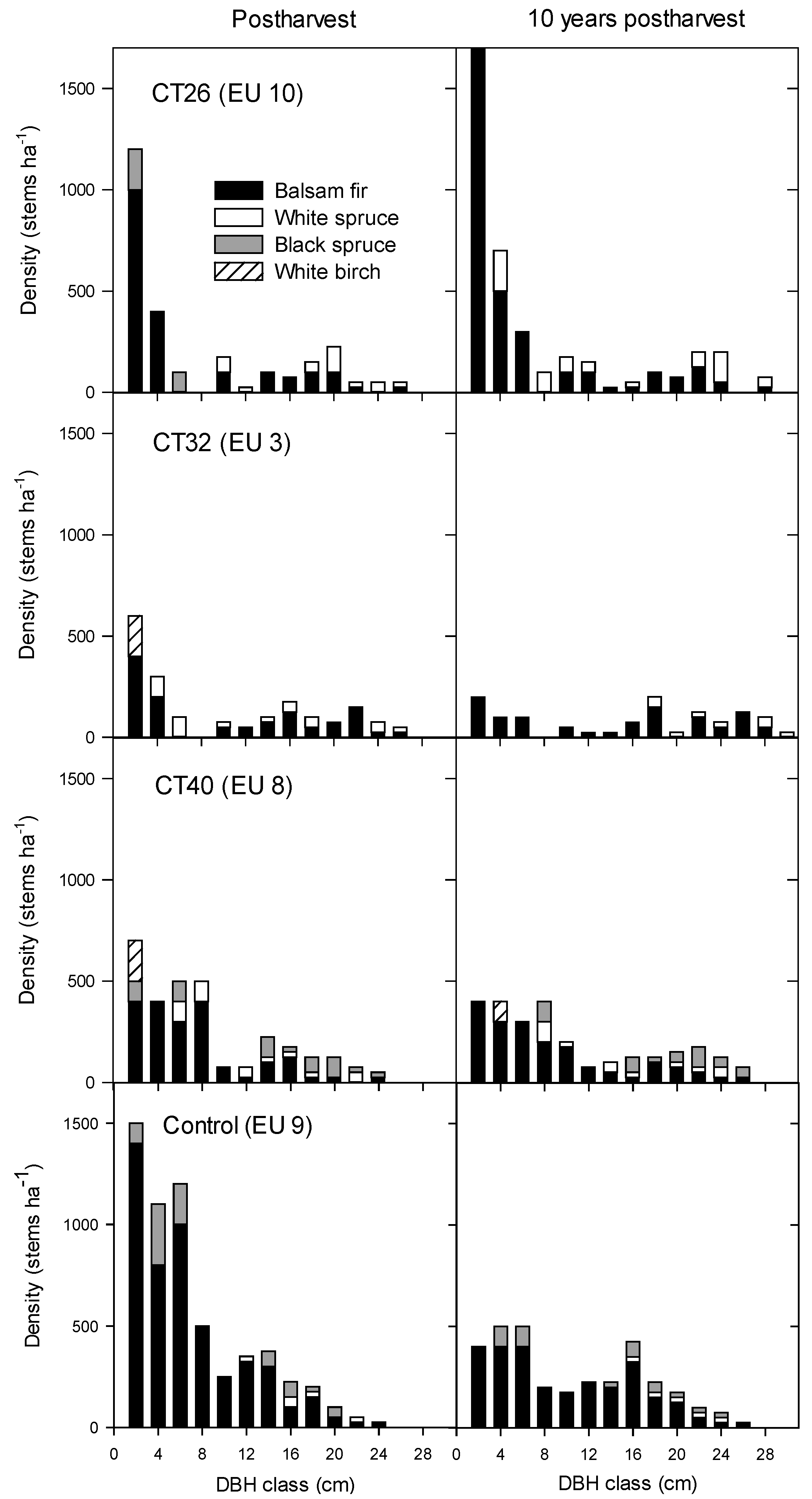
3.2.2. Regeneration Density and Stocking


4. Discussion
4.1. Growth and Yield
4.1.1. Mean Tree Level
4.1.2. Stand Level
4.2. Structural Heterogeneity
4.2.1. Number of Large Trees and Shape of the Diameter Distribution
4.2.2. Regeneration Density and Stocking
5. Conclusions
Acknowledgments
Author Contributions
Supplementary


Conflicts of Interest
References
- Schütz, J.P.; Pukkala, T.; Donoso, P.J.; von Gadow, K. Historical emergence and current application of CCF. In Continuous Cover Forestry, 2nd ed.; Pukkala, T., von Gadow, K., Eds.; Springer: Dordrecht, The Netherlands, 2012; pp. 1–28. [Google Scholar]
- Simpson, J. 1903.; The New Forestry, 2nd ed.; Pawson & Brailsford Ltd: Sheffield, UK, 1903; p. 220. [Google Scholar]
- Kerr, G. The use of silvicultural systems to enhance the biological diversity of plantation forests in Britain. Forestry 1999, 72, 191–205. [Google Scholar] [CrossRef]
- Franklin, J.F. Toward a new forestry. Am. For. 1989, 95, 37–44. [Google Scholar]
- Seymour, R.S.; Hunter, M.L. New forestry in eastern spruce-fir forests: Principles and applications to Maine; Maine Agricultural and Forest Experiment Station Miscellaneous: Orono, ME, USA, 1992; p. 36. [Google Scholar]
- Lorimer, C.G.; Freelich, L.E. Natural disturbance regimes for old-growth northern hardwoods: Implications for restoration efforts. J. For. 1994, 92, 33–38. [Google Scholar]
- Oliver, C.; Larson, B. Forest Stand Dynamics, 2nd ed.; Wiley: New York, NY, USA, 1996; p. 520. [Google Scholar]
- O’Hara, K.L. Silviculture for structural diversity: A new look at multiaged systems. J. For. 1998, 96, 4–10. [Google Scholar]
- Landres, P.B.; Morgan, P.; Swanson, F.J. Overview of the use of natural variability concepts in managing ecological systems. Ecol. Appl. 1999, 9, 1179–1188. [Google Scholar]
- O’Hara, K.L.; Ramage, B.S. Silviculture in an uncertain world: Utilizing multi-aged management systems to integrate disturbance. Forestry 2013, 86, 401–410. [Google Scholar] [CrossRef]
- Gauthier, S.; Vaillancourt, M.A.; Kneeshaw, D.; Drapeau, P.; de Granpré, L.; Claveau, Y.; Paré, D. Aménagement écosystémique: Origines et fondements. In Aménagement Ecosystémique en Forêt Boréale; Presses del’Université du Québec: Québec, Canada, 2008; pp. 11–40. [Google Scholar]
- Boucher, Y.; Arseneault, D.; Sirois, L.; Blais, L. Logging pattern and landscape changes over the last century at the boreal and deciduous forest transition in Eastern Canada. Landsc. Ecol. 2009, 24, 171–184. [Google Scholar] [CrossRef]
- Puettmann, K.J.; Coates, K.D.; Messier, C. A Critique of Silviculture: Managing Complexity; Island Press: Washington, DC, USA, 2008; p. 208. [Google Scholar]
- Arielle Angers, V.; Messier, C.; Beaudet, M.; Leduc, A. Comparing composition and structure in old-growth and harvested (selection and diameter-limit cuts) northern hardwood stands in Quebec. For. Ecol. Manag. 2005, 217, 275–293. [Google Scholar] [CrossRef] [Green Version]
- Bauhus, J.; Puettmann, K.; Messier, C. Silviculture for old-growth attributes. For. Ecol. Manag. 2009, 258, 525–537. [Google Scholar] [CrossRef] [Green Version]
- Schütz, J.P. Opportunities and strategies of transforming regular forests to irregular forests. For. Ecol. Manag. 2001, 151, 87–94. [Google Scholar] [CrossRef]
- Singer, M.T.; Lorimer, C.G. Crown release as a potential old-growth restoration approach in northern hardwoods. Can. J. For. Res. 1997, 27, 1222–1232. [Google Scholar] [CrossRef]
- Lindh, B.C.; Muir, P.S. Understory vegetation in young Douglas-fir forest: Does thinning help restore old–growth composition? For. Ecol. Manag. 2004, 192, 285–296. [Google Scholar] [CrossRef]
- Sullivan, T.P.; Sullivan, D.S.; Lindgren, P.M.F.; Ransome, D.B. Long-term responses of ecosystem components to stand thinning in young lodgepole pine forest. III Growth of crop trees and coniferous stand structure. For. Ecol. Manag. 2006, 228, 69–81. [Google Scholar] [CrossRef]
- Choi, J.; Lorimer, C.G.; Vanderwerker, J.M. A simulation of the development and restoration of old–growth structural features in northern hardwoods. For. Ecol. Manag. 2007, 249, 204–220. [Google Scholar] [CrossRef]
- O’Hara, K.L.; Leonard, L.P.; Keyes, C.R. Variable–Density thinning and a marking paradox: Comparing prescription protocols to attain stand variability in coast redwood. West. J. Appl. For. 2012, 27, 143–149. [Google Scholar] [CrossRef]
- Drössler, L.; Nilsson, U.; Lundqvist, L. Simulated transformation of even-aged Norway spruce stands to multi–layered forests: An experiment to explore the potential of tree size differentiation. Forestry 2014, 87, 239–248. [Google Scholar] [CrossRef]
- Assmann, E. The Principles of Forest Yield Study; Pergamon Press Ltd: New York, NY, USA, 1970; p. 506. [Google Scholar]
- Ministère des Ressources Naturelles (MRN). Avis Scientifique: Éclaircie Commerciale Pour le Groupe de Production Prioritaire SEPM; Gouv du Québec, Ministère des Ressources Naturelles (MRN): Quebec City, QC, Canada, 2003; p. 80. [Google Scholar]
- Busing, R.T.; Garman, S.L. Promoting old–growth characteristics and long-term wood production in Douglas–fir forests. For. Ecol. Manag. 2002, 160, 161–175. [Google Scholar] [CrossRef]
- Lafond, V.; Cordonnier, T.; de Coligny, F.; Courbaud, B. Reconstructing harvesting diameter distribution from aggregate data. Ann. For. Sci. 2012, 69, 235–243. [Google Scholar] [CrossRef]
- Boulanger, Y.; Arseneault, D. Spruce budworm outbreaks in eastern Quebec over the last 450 years. Can. J. For. Res. 2004, 34, 1035–1043. [Google Scholar] [CrossRef]
- Frank, R.M.; Bjorkbom, J.C. A silvicultural guide to spruce-fir in the northeast. In Gen. Tech. Rep. NE-6; USDA Forestry Service.: Asheville, NC, USA, 1973; p. 29. [Google Scholar]
- Bégin, E.; Bégin, J.; Bélanger, L.; Rivest, L.P.; Tremblay, S. Balsam fir self-thinning relationship and its constancy among different ecological regions. Can. J. For. Res. 2001, 31, 950–959. [Google Scholar] [CrossRef]
- Pothier, D.; Savard, F. Actualisation des Tables de Production Pour les Principales Espèces Forestières du Québec; Gouv Québec, Min. Ress. Nat., Dir. Inv. For., Ministère des Ressources naturelles: Québec, Canada, 1998; p. 183. [Google Scholar]
- Zeide, B.L. Thinning and growth: a full turnaround. J. For. 2001, 99, 20–25. [Google Scholar]
- Fortin, M.; Bernier, S.; Saucier, J.P.; Labbé, F. Une relation hauteur–diamètre tenant compte de l’influence de la station et du climat pour 20 espèces commerciales du Québec. In Mathieu Fortin; Direction de la recherche forestière: Québec, Canada, 2009; p. 22. [Google Scholar]
- Fortin, M.; DeBlois, J.; Bernier, S.; Blais, G. Mise au point d’un tarif de cubage général pour les forêts québécoises: Une approche pour mieux évaluer l’incertitude associée aux prévisions. For. Chron. 2007, 83, 754–765. [Google Scholar] [CrossRef]
- Nappi, A.; Drapeau, P. Pre–fire forest conditions and fire severity as determinants of the quality of burned forests for deadwood-dependent species: The case of the black-backed woodpecker. Can. J. For. Res. 2011, 41, 994–1003. [Google Scholar] [CrossRef]
- McCarthy, J.W.; Weetman, G. Stand structure and development of an insect–mediated boreal forest landscape. For. Ecol. Manag. 2007a, 241, 101–114. [Google Scholar]
- McCarthy, J.W.; Weetman, G. Self–thinning dynamics in a balsam fir (Abies balsamea (L.) Mill.) insect-mediated boreal forest chronosequence. For. Ecol. Manag. 2007b, 241, 295–309. [Google Scholar]
- Ruel, J.C.; Fortin, D.; Pothier, D. Partial cutting in old-growth boreal stands: An integrated experiment. For. Chron. 2013, 89, 360–369. [Google Scholar] [CrossRef]
- Brown, H.; Prescott, R. Applied Mixed Models in Medicine, 2nd ed.; John Wiley & Sons, Inc: Chichester, UK, 2006; p. 455. [Google Scholar]
- Mead, R. The Design of Experiments-Statistical Principles for Practical Application; Cambridge University Press: New York, NY, USA, 1988; p. 620. [Google Scholar]
- Littell, R.C.; Milliken, G.A.; Stroup, W.W.; Wolfinger, R.D.; Schabenberger, O. SAS for Mixed Models, 2nd ed.; SAS Institute: Cary, NC, USA, 2006; p. 814. [Google Scholar]
- Westfall, P.H.; Tobias, R.D.; Wolfinger, R.D. Multiple Comparisons and Multiple Tests Using SAS, 2nd ed.; SAS Institute: Cary, NC, USA, 2011; p. 625. [Google Scholar]
- Côté, G.; Bouchard, M.; Pothier, D.; Gauthier, S. Linking stand attributes to cartographic information for ecosystem management purposes in the boreal forest of eastern Québec. For. Chron. 2010, 86, 511–519. [Google Scholar] [CrossRef]
- Barrette, M.; Bélanger, L. Reconstitution historique du paysage préindustriel de la région écologique des hautes collines du Bas-Saint-Maurice. Can. J. For. Res. 2007, 37, 1147–1160. [Google Scholar] [CrossRef]
- Bailey, R.L.; Dell, T.R. Quantifying diameter distributions with the Weibull function. For. Sci. 1973, 19, 97–104. [Google Scholar]
- Wyszomirski, T. Detecting and displaying size bimodality: Kuz trtosis, skewness and bimodalizable distributions. J. Theor. Biol. 1992, 158, 109–128. [Google Scholar] [CrossRef]
- Lorimer, C.G.; Krug, A.G. Diameter distributions in even–aged stands of shade-tolerant and midtolerant tree species. Am. Midl. Nat. 1983, 109, 331–345. [Google Scholar] [CrossRef]
- Ruel, J.C.; Doucet, R.; Boily, J. Mortality of balsam fir and black spruce advance growth 3 years after clear-cutting. Can. J. For. Res. 1995, 25, 1528–1537. [Google Scholar] [CrossRef]
- Ministry of Forests. Guidelines for Developing Stand Density Management Regimes; British Columbia Ministry Forestry, Forestry Practices British: Victoria, Canada, 1999; p. 94. [Google Scholar]
- Büsgen, M.; Münch, E. The Structure and Life of Forest Trees; Chapman & Hall Ltd: London, UK, 1929; p. 436. [Google Scholar]
- Schlesinger, R.C. Increased growth of released white oak poles continues through two decades. J. For. 1978, 76, 726–727. [Google Scholar]
- Ward, J.S. Crop tree release increases growth of mature red oak sawtimber. North J. Appl. For. 2002, 19, 149–154. [Google Scholar]
- Pelletier, G.; Pitt, D.G. Silvicultural responses of two spruce plantations to midrotation commercial thinning in New Brunswick. Can. J. For. Res. 2008, 38, 851–867. [Google Scholar] [CrossRef]
- Krause, C.; Laplante, S.; Plourde, P.Y. Transversal tracheid dimension in thinned black spruce and Jack pine stands in the boreal forest. Scand. J. For. Res. 2011, 26, 477–487. [Google Scholar] [CrossRef]
- Gagné, L.; Lavoie, L.; Binot, J.M. Croissance et propriétés mécaniques du bois après éclaircie commerciale dans une plantation d’épinette blanche (Picea glauca) âgée de 32 ans. Can. J. For. Res. 2012, 42, 291–302. [Google Scholar] [CrossRef]
- Poulin, J. Bureau du forestier en chef. Manuel de détermination des possibilités forestières 2013–2018. In Fascicule 35; Gouv. Québec: Roberval, Canada, 2013; pp. 95–98. [Google Scholar]
- Coates, K.D. Windthrow damage 2 years after partial cutting at the Date Creek silvicultural systems study in the Interior Cedar–Hemlock forests of Northwestern British Columbia. Can. J. For. Res. 1997, 27, 1695–1701. [Google Scholar] [CrossRef]
- Nilsson, U.; Agestam, E.; Ekö, P.M.; Elfving, B.; Fahlvik, N.; Johansson, U.; Karlsson, K.; Lundmark, T.; Wallentin, C. Thinning of Scots pine and Norway spruce monocultures in Sweden -Effects of different thinning programmes on stand level gross-and net stem volume production. Stud. For. Suec. 2010, 219, 46. [Google Scholar]
- Carey, A.B. Bioheterogeneity and restoration of biodiversity in temperate coniferous forest: Inducing spatial heterogeneity with variable-density thinning. Forestry 2003, 76, 127–136. [Google Scholar] [CrossRef]
- Mäkinen, H.; Isomäki, A. Thinning intensity and long-term changes in increment and stem form of Norway spruce trees. For. Ecol. Manag. 2004a, 201, 295–309. [Google Scholar] [CrossRef]
- Mäkinen, H.; Isomäki, A. Thinning intensity and long-term changes in increment and stem form of Scots pine trees. For. Ecol. Manag. 2004b, 203, 21–34. [Google Scholar] [CrossRef]
- Lindenmayer, D.B.; Franklin, J.F.; Fisher, J. General management principles and a checklist of strategies to guide forest biodiversity conservation. Biol. Conserv. 2006, 131, 433–445. [Google Scholar] [CrossRef]
- Gamfeldt, L.; Snäll, T.; Bagchi, R.; Jonsson, M.; Gustafsson, L.; Kjellander, P.; Ruiz-Jaen, M.C.; Fröberg, M.; Stendahl, J.; Philipson, C.D.; et al. Higher levels of multiple ecosystem services are found in forests with more tree species. Nat. Commun. 2013, 4, 1340. [Google Scholar] [CrossRef] [PubMed] [Green Version]
- Sullivan, T.P.; Sullivan, D.S.; Lindgren, P.M.F.; Ransome, D.B. Stand structure and the abundance and diversity of plants and small mammals in natural and intensively managed forests. For. Ecol. Manag. 2009, 258S, S127–S141. [Google Scholar] [CrossRef]
- Barrette, M.; Bélanger, L.; de Grandpré, L. Preindustrial reconstruction of a perhumid midboreal landscape, Anticosti Island, Quebec. Can. J. For. Res. 2010, 40, 928–942. [Google Scholar] [CrossRef]
- Olson, M.G.; Meyer, S.R.; Wagner, R.G.; Seymour, R.S. Commercial thinning stimulates natural regeneration in spruce-fir stands. Can. J. For. Res. 2014, 44, 173–181. [Google Scholar] [CrossRef]
- Pothier, D. Évolution de la régénération après la coupe de peuplements récoltés selon différents procédés d’exploitation. For. Chron. 1996, 72, 519–527. [Google Scholar] [CrossRef]
- Bataineh, M.M.; Kenefic, L.S.; Weiskittel, A.R.; Wagner, R.G.; Bissette, J.C. Influence of partial harvesting and site factors on the abundance and composition of natural regeneration in the Acadian Forest of Maine, USA. For. Ecol. Manag. 2013, 306, 96–106. [Google Scholar] [CrossRef]
- Ares, A.; Neill, A.R.; Puettmann, K.J. Understory abundance, species diversity and functional attribute response to thinning in coniferous stands. For. Ecol. Manag. 2010, 260, 1104–1113. [Google Scholar] [CrossRef]
© 2015 by the authors; licensee MDPI, Basel, Switzerland. This article is an open access article distributed under the terms and conditions of the Creative Commons Attribution license (http://creativecommons.org/licenses/by/4.0/).
Share and Cite
Gauthier, M.-M.; Barrette, M.; Tremblay, S. Commercial Thinning to Meet Wood Production Objectives and Develop Structural Heterogeneity: A Case Study in the Spruce-Fir Forest, Quebec, Canada. Forests 2015, 6, 510-532. https://doi.org/10.3390/f6020510
Gauthier M-M, Barrette M, Tremblay S. Commercial Thinning to Meet Wood Production Objectives and Develop Structural Heterogeneity: A Case Study in the Spruce-Fir Forest, Quebec, Canada. Forests. 2015; 6(2):510-532. https://doi.org/10.3390/f6020510
Chicago/Turabian StyleGauthier, Martin-Michel, Martin Barrette, and Stéphane Tremblay. 2015. "Commercial Thinning to Meet Wood Production Objectives and Develop Structural Heterogeneity: A Case Study in the Spruce-Fir Forest, Quebec, Canada" Forests 6, no. 2: 510-532. https://doi.org/10.3390/f6020510