Low-Density LiDAR and Optical Imagery for Biomass Estimation over Boreal Forest in Sweden


Abstract
:
1. Introduction
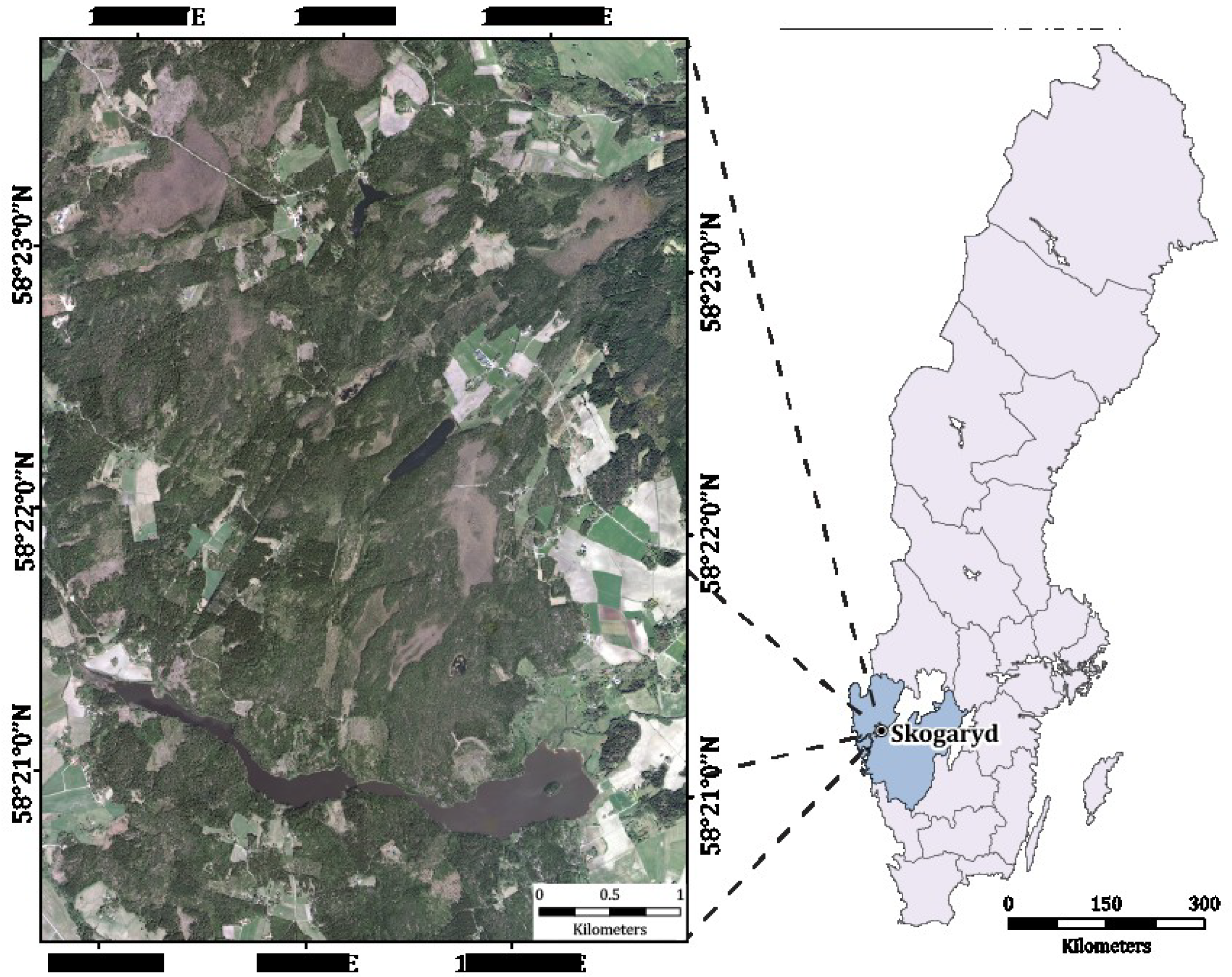
2. Study Area
3. Data and Methods
3.1. Field Measurements
3.2. Remotely Sensed Data
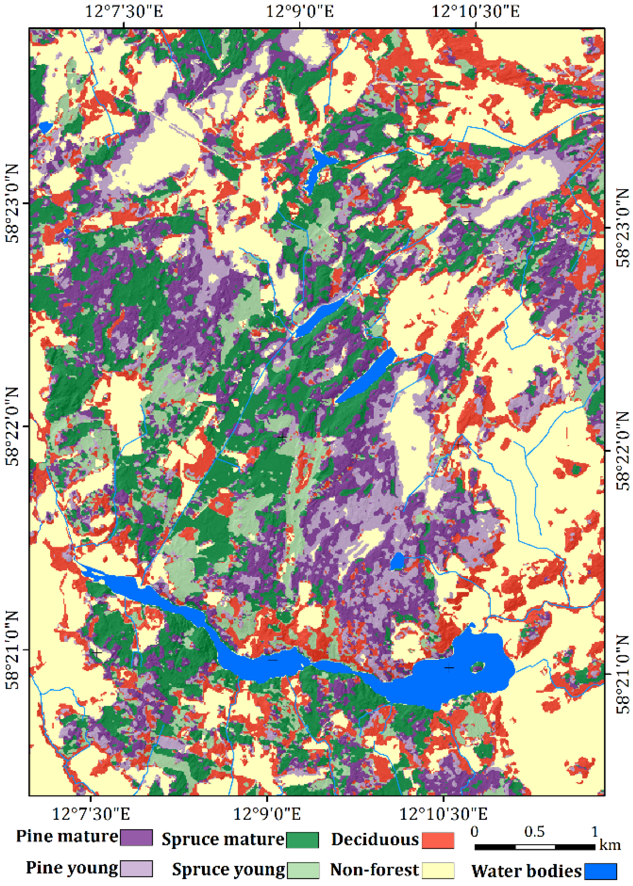
3.3. Vegetation Mapping Using Maximum-Likelihood Classification
3.4. Derivation of Amount of Trees and Their Heights from Airborne LiDAR
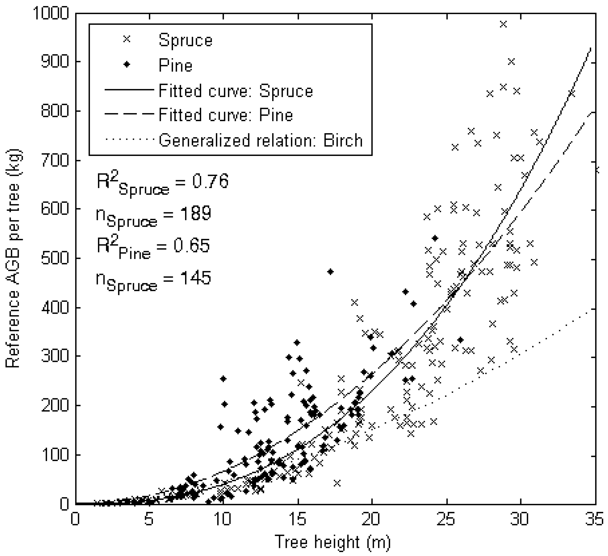
3.5. Reference Biomass Estimation

| Biomass (kg) | DBH | H | n | R2 | Equation | a | b | c | d | |
|---|---|---|---|---|---|---|---|---|---|---|
| Spruce | ln(CR) | cm | - | 544 | 0.95 | a + b × [DBH/(DBH + 13)] | −1.280 | 8.524 | - | - |
| Spruce | ln(CR) | cm | m | 544 | 0.95 | a + b × [DBH/(DBH + 13)] + c × H + d × ln(H) | −1.206 | 10.971 | −0.012 | −0.492 |
| Spruce | ln(ST) | cm | - | 546 | 0.99 | a + b × [DBH/(DBH + 14)] | −2.057 | 11.334 | - | - |
| Spruce | ln(ST) | cm | m | 546 | 0.99 | a + b × [DBH/(DBH + 14)] + c × H + d × ln(H) | −2.170 | 7.469 | 0.029 | 0.686 |
| Pine | ln(CR) | cm | - | 482 | 0.90 | a + b ×[DBH/(DBH + 10)] | −2.860 | 9.102 | - | - |
| Pine | ln(CR) | cm | m | 482 | 0.92 | a + b·[DBH/(DBH + 10)] + c × ln(H) | −2.541 | 13.396 | −1.196 | - |
| Pine | ln(ST) | cm | - | 488 | 0.98 | a + b × [DBH/(DBH + 13)] | −2.339 | 11.326 | - | - |
| Pine | ln(ST) | cm | m | 488 | 0.99 | a + b × [DBH/(DBH + 13)] + c × H + d × ln(H) | −2.677 | 7.594 | 0.015 | 0.880 |
| Birch | AGB | mm | - | - | 0.99 | a × DBH b | 0.0009 | 2.2864 | - | - |
4. Results and Discussion
4.1. Vegetation Classes
| Spruce Mature | Spruce Young | Pine Mature | Pine Young | Deciduous | Total | Producer’s accuracy (%) | Area (km2) | Area (%) | |
|---|---|---|---|---|---|---|---|---|---|
| Spruce Mature | 67 | 3 | 5 | 0 | 1 | 76 | 92 | 5.4 | 26.6 |
| Spruce Young | 2 | 25 | 3 | 0 | 1 | 31 | 86 | 2.5 | 12.3 |
| Pine Mature | 4 | 1 | 32 | 8 | 0 | 45 | 68 | 4.6 | 22.7 |
| Pine Young | 0 | 0 | 7 | 10 | 0 | 17 | 50 | 3.2 | 15.7 |
| Deciduous | 0 | 0 | 0 | 2 | 25 | 27 | 93 | 4.6 | 22.7 |
| Total | 73 | 29 | 47 | 20 | 27 | 196 | |||
| User’s accuracy (%) | 88 | 81 | 71 | 59 | 93 | Total accuracy (%) | 81 | ||
| Kappa coefficient | 0.75 | ||||||||

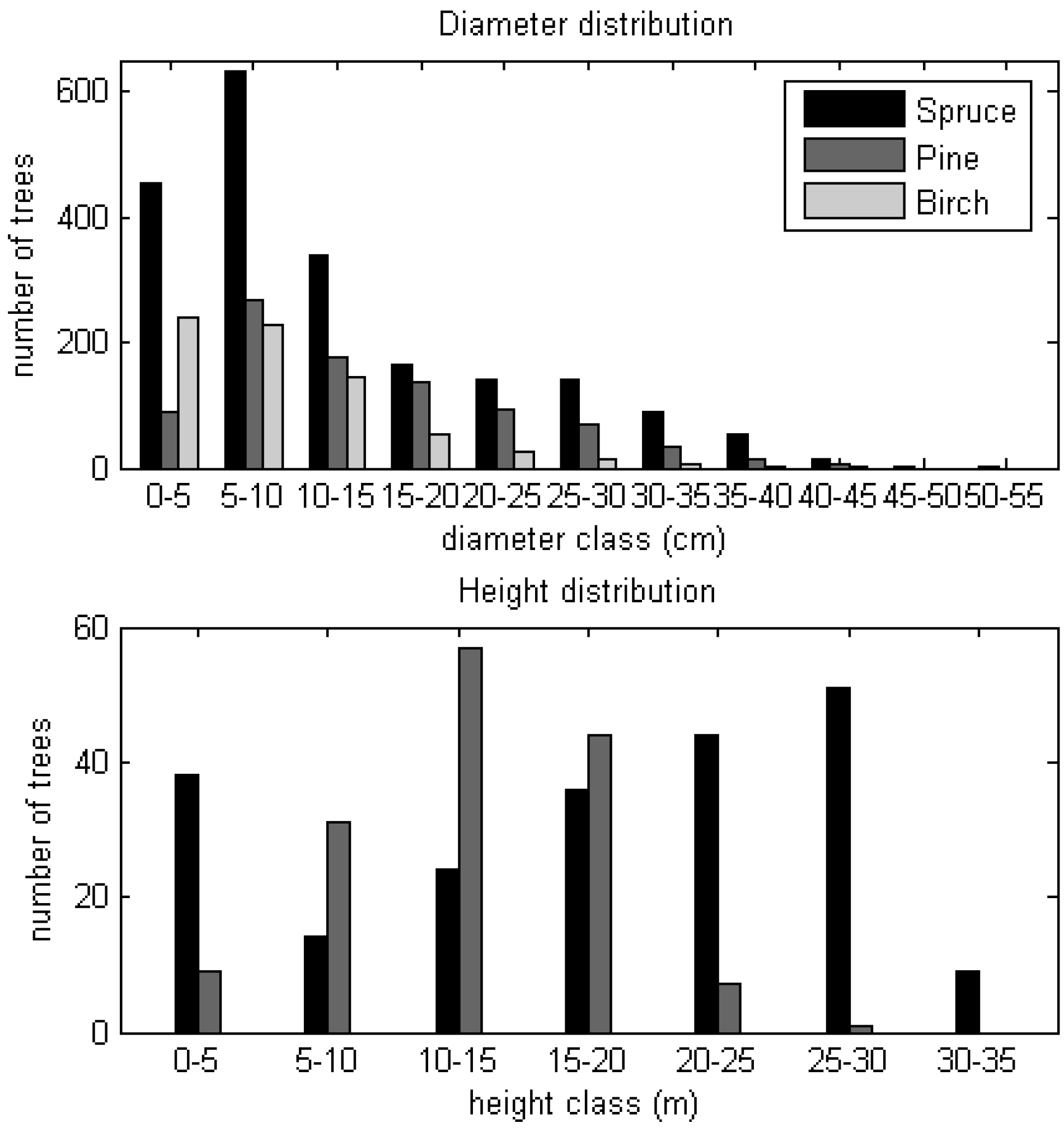
4.2. Reference Aboveground Biomass Estimates

4.3. LiDAR-Derived Forest Inventory Parameters
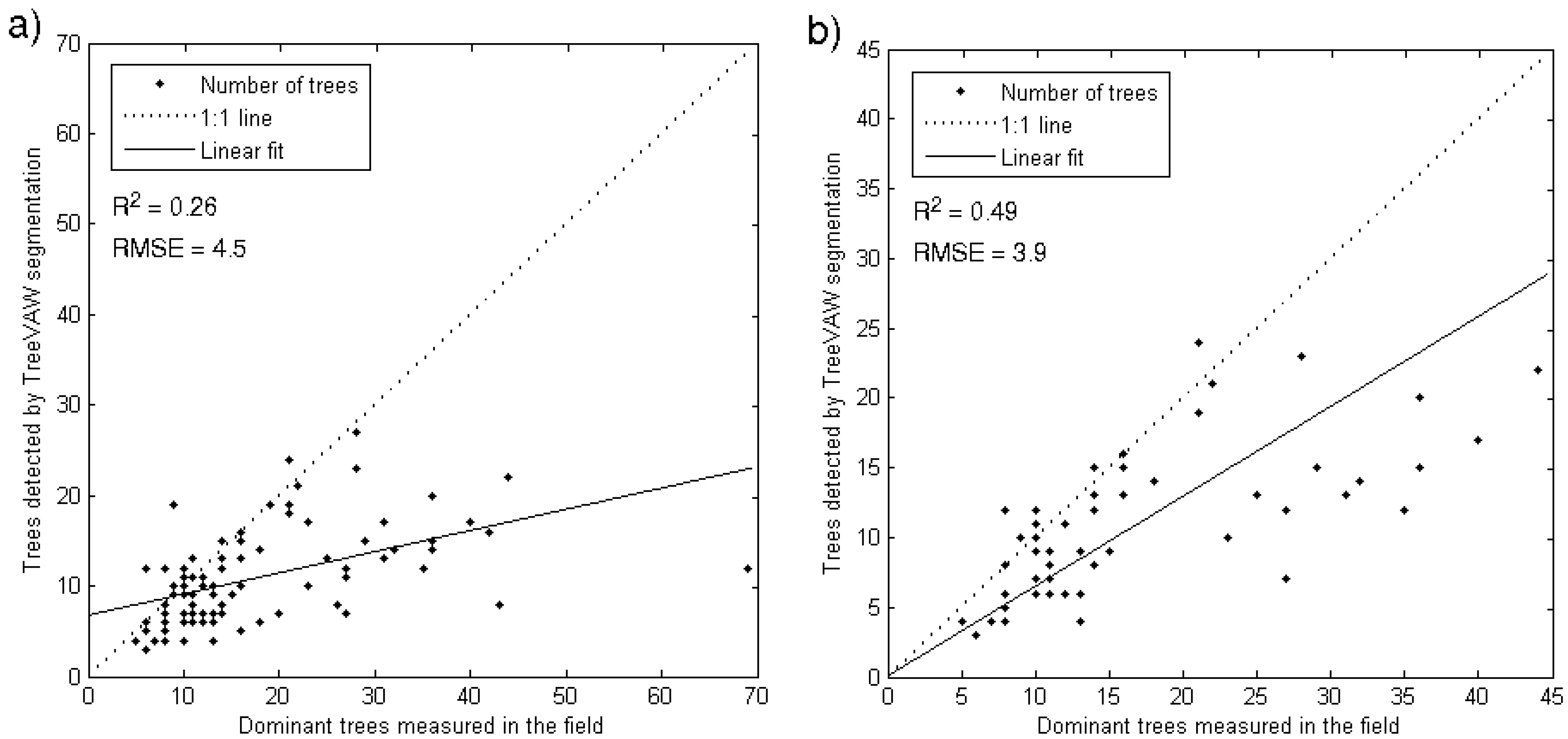
4.3.1. Tree Density
4.3.2. Tree Height

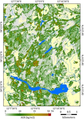
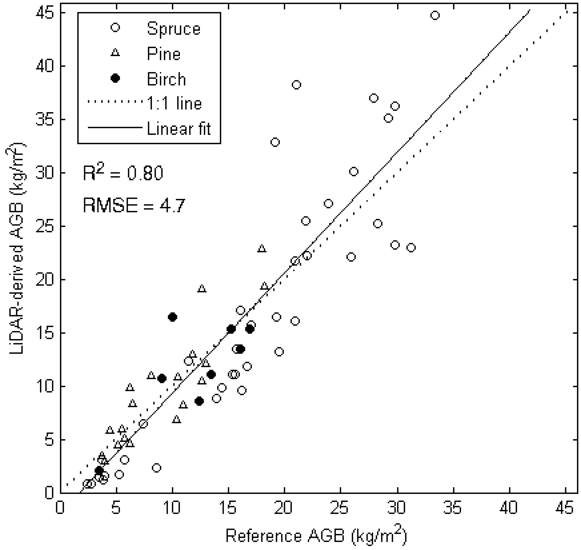
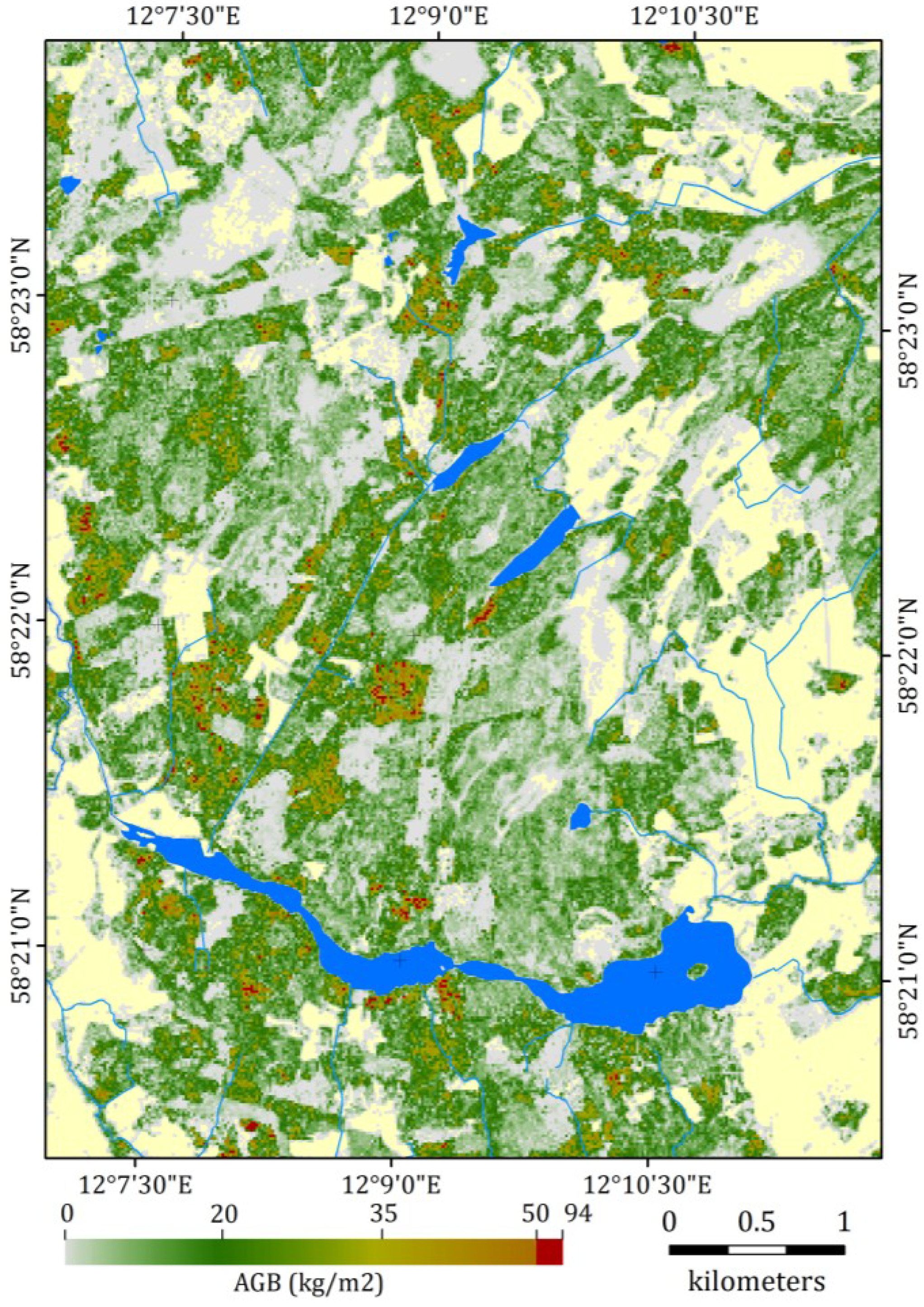
4.4. Aboveground Biomass Estimates over the Study Area


5. Conclusions
Acknowledgments
Author Contributions
Conflicts of Interest
References and Notes
- IPCC. Climate Change 2007: Mitigation of Climate Change. IPCC Fourth Assessment Report (AR4); Contribution of Working Group III to the Fourth Assessment Report of the Intergovernmental Panel on Climate Change, 2007; Metz, B., Davidson, O.R., Bosch, P.R., Dave, R., Meyer, L.A., Eds.; Cambridge University Press: Cambridge, UK, 2007. [Google Scholar]
- Houghton, R.A.; Hall, F.; Goetz, S.J. Importance of biomass in the global carbon cycle. J. Geophys. Res. 2009, 114, 1–13. [Google Scholar]
- Lefsky, M.A.; Cohen, W.B.; Harding, D.J.; Parker, G.G.; Acker, S.A.; Gower, S.T. LiDAR remote sensing of aboveground biomass in three biomes. Glob. Ecol. Biogeogr. 2002, 11, 393–399. [Google Scholar] [CrossRef]
- Maltamo, M.; Mustonen, K.; Hyyppä, J.; Pitkänen, J.; Yu, X. The accuracy of estimating individual tree variables with airborne laser scanning in a boreal nature reserve. Can. J. For. Res. 2004, 34, 1791–1801. [Google Scholar] [CrossRef]
- Hese, S.; Lucht, W.; Schmullius, C. Global biomass mapping for an improved understanding of the CO2 balance-the Earth observation mission carbon-3D. Remote Sens. Environ. 2005, 94, 94–104. [Google Scholar] [CrossRef]
- Nord-Larsen, T.; Shumacher, J. Estimation of forest resources from a country wide laser scanning survey and national forest inventory data. Remote Sens. Environ. 2012, 119, 148–157. [Google Scholar] [CrossRef]
- Popescu, S.C. Estimating biomass of individual pine trees using airborne LiDAR. Biomass Bioenergy 2007, 31, 646–655. [Google Scholar] [CrossRef]
- Bortolot, Z.J.; Wynne, R.H. Estimating forest biomass using small footprint LiDAR data: An individual tree-based approach that incorporates training data. ISPRS J. Photogramm. Remote Sens. 2005, 59, 342–360. [Google Scholar] [CrossRef]
- Chen, Q.; Laurin, G.V.; Battles, J.J.; Saah, D. Integration of airborne LiDAR and vegetation types derived from aerial photography for mapping aboveground live biomass. Remote Sens. Environ. 2012, 121, 108–117. [Google Scholar] [CrossRef]
- Evans, J.S.; Hudak, A.T.; Faux, R.; Smith, A.M.S. Discrete return LiDAR in natural resources: Recommendations for project planning, data processing, and deliverables. Remote Sens. 2009, 1, 776–794. [Google Scholar] [CrossRef]
- Hopkinson, C.; Chasmer, L.; Colville, D.; Fournier, R.A.; Hall, R.J.; Luther, J.E.; Milne, T.; Petrone, R.M.; St-onge, B. Moving toward consistent ALS monitoring of forest attributes across Canada: A consortium approach. Photogramm. Eng. Remote Sens. 2013, 79, 159–173. [Google Scholar] [CrossRef]
- Jochem, A.; Hollaus, M.; Rutzinger, M.; Höfle, B. Estimation of aboveground biomass in alpine forests: A semi-empirical approach considering canopy transparency derived from airborne LiDAR data. Sensors 2011, 11, 278–295. [Google Scholar]
- Luther, J.E.; Skinner, R.; Fournier, R.A.; van Lier, O.R.; Bowers, W.W.; Cote, J.F.; Hopkinson, C.; Moulton, T. Predicting wood quantity and quality attributes of balsam fir and black spruce using airborne laser scanner data. Forestry 2014, 87, 313–326. [Google Scholar]
- Ramdani, F. Urban vegetation mapping from fused hyperspectral image and LiDAR data with application to monitor urban tree heights. J. Geogr. Inf. Syst. 2013, 5, 404–408. [Google Scholar]
- Lin, Y.; Jaakkola, A.; Hyyppä, J.; Kaartinen, H. From TLS to VLS: Biomass estimation at individual tree level. Remote Sens. 2010, 2, 1864–1879. [Google Scholar] [CrossRef]
- Edson, C.; Wing, M.G. Airborne light detection and ranging (LiDAR) for individual tree stem location, height, and biomass measurements. Remote Sens. 2011, 3, 2494–2528. [Google Scholar] [CrossRef] [Green Version]
- Zianis, D.; Muukkonen, P.; Mäkipää, R.; Mencuccini, M. Biomass and stem volume equations for tree species in Europe. Silva Fenn. Monogr. 2005, 4, 1–63. [Google Scholar]
- Andersen, H.E.; Strunk, J.; Temesgcn, H.; Atwood, D.; Winterberger, K. Using multilevel remote sensing and ground data to estimate forest biomass resources in remote regions: A case study in the boreal forests of interior Alaska. Can. J. Remote Sens. 2011, 37, 1–16. [Google Scholar]
- Meyer, A.; Tarvainen, L.; Nousratpour, A.; Björk, R.G.; Ernfors, M.; Grelle, A.; Klemedtsson, Å.K.; Lindroth, A.; Räntfors, M.; Rütting, T.; Wallin, G.; Weslien, P.; Klemedtsson, L.A. Fertile peatland forest does not constitute a major greenhouse gas sink. Biogeosciences 2013, 10, 7739–7758. [Google Scholar] [CrossRef]
- Vertex IV; Vertex IV and Transponder T3 Manual 2007. Vertex: Långsele, Sweden, 2007. Available online: http://www.haglofcg.com/index.php?option=com_content&view=article&id=49&Itemid=82&lang=en (accessed on 10 January).
- Bucksch, A.; Lindenbergh, R.; Menenti, M. Robust skeleton extraction from imperfect point clouds. Vis. Comput. 2010, 26, 1283–1300. [Google Scholar] [CrossRef]
- Lantmäteriet. Produktbeskrivning Laserdata, Dokumentversion: 1.6. Available online: http://www.lantmateriet.se/Global/Kartor%20och%20geografisk%20information/H%C3%B6jddata/Produktbeskrivningar/laserdat.pdf (accessed on 12 December 2012).
- Mehner, H.; Cutler, M.; Fairbairn, D.; Thompson, G. Remote sensing of upland vegetation: The potential of high spatial resolution satellite sensors. Glob. Ecol. Biogeogr. 2004, 13, 359–369. [Google Scholar] [CrossRef]
- Congalton, R.G. A review of assessing the accuracy of classifications of remotely sensed data. Remote Sens. Environ. 1991, 37, 35–46. [Google Scholar] [CrossRef]
- MARS Explorer, Mars 7.1 Help Manual 2012; MARS: Greenwood Village, CO, USA, 2012.
- Popescu, S.C.; Wynne, R.H. Seeing the trees in the forest: Using LiDAR and multispectral data fusion with local filtering and variable window size for estimating tree height. Photogramm. Eng. Remote Sens. 2004, 70, 589–604. [Google Scholar] [CrossRef]
- Marklund, L.G. Biomassafunktioner för tall, gran och björk i Sverige. Sveriges Lantbruksuniversitet, Institutionen för Skogstaxering. Rapport 1988, 45, 1–73. (in Swedish). [Google Scholar]
- Johansson, T. Biomass equations for determining functions of pendula and pubescent birches growing on abandoned farmland and some practical implications. Biomass Bioenergy 1999, 16, 223–238. [Google Scholar] [CrossRef]
- Lieffers, V.J.; Stadt, K.J.; Navratil, S. Age structure and growth of understory white spruce under aspen. Can. J. For. Res. 1996, 26, 1002–1007. [Google Scholar] [CrossRef]
- Mette, T.; Papathanassiou, K.; Hajnsek, I. Biomass estimation from polarimetric SAR interferometry over heterogeneous forest terrain. In Geoscience and Remote Sensing Symposium, 2004. IGARSS '04. Proceedings. 2004 IEEE International, Anchorage, AK, USA, 20–24 September 2004; pp. 511–514.
- Mette, T. Forest Biomass Estimation from Polarimetric SAR Interferometry. Ph.D. Thesis, Center of Life and Food Sciences Weihenstephan, Technical University of Munich, Munich, Germany, 2006. [Google Scholar]
- Mehtätalo, L. Height-Diameter Models for Scots Pine and Birch in Finland. Silva Fennica 2005, 39, 55–66. [Google Scholar]
- Gebreslasie, M.T.; Ahmed, F.B.; van Aardt, J.A.N.; Blakeway, F. Individual tree detection based on variable and fixed window size local maxima filtering applied to IKONOS imagery for even-aged Eucalyptus plantation forests. Int. J. Remote Sens. 2011, 32, 4141–4154. [Google Scholar] [CrossRef]
- Morsdorf, F.; Meier, E.; Kötz, B.; Itten, K.I.; Dobbertin, M.; Allgöwer, B. Lidar-based geometric reconstruction of boreal type forest stands at single tree level for forest and wildland fire management. Remote Sens. Environ. 2004, 92, 353–362. [Google Scholar] [CrossRef]
- Roberts, S.D.; Dean, T.J.; Evans, D.L.; McCombs, J.W.; Harrington, R.L.; Glass, P.A. Estimating individual tree leaf area in loblolly pine plantations using LiDAR-derived measurements of height and crown dimensions. For. Ecol. Manag. 2005, 213, 54–70. [Google Scholar] [CrossRef]
- Zimble, D.A.; Evans, D.L.; Carlson, G.C.; Parker, R.C.; Grado, S.C.; Gerard, P.D. Characterising vertical forest structure using small-footprint airborne LiDAR. Remote Sens. Environ. 2003, 87, 171–182. [Google Scholar] [CrossRef]
- Whittaker, R.H. Communities and Ecosystems, 2nd ed.; MacMillan Publishing: New York, NY, USA, 1975. [Google Scholar]
- Available online: www.cec.lu.se/research/becc (accessed on 10 January 2014).
- Available online: www.lucci.lu.se (accessed on 10 January 2014).
© 2014 by the authors; licensee MDPI, Basel, Switzerland. This article is an open access article distributed under the terms and conditions of the Creative Commons Attribution license (http://creativecommons.org/licenses/by/3.0/).
Share and Cite
Shendryk, I.; Hellström, M.; Klemedtsson, L.; Kljun, N. Low-Density LiDAR and Optical Imagery for Biomass Estimation over Boreal Forest in Sweden. Forests 2014, 5, 992-1010. https://doi.org/10.3390/f5050992
Shendryk I, Hellström M, Klemedtsson L, Kljun N. Low-Density LiDAR and Optical Imagery for Biomass Estimation over Boreal Forest in Sweden. Forests. 2014; 5(5):992-1010. https://doi.org/10.3390/f5050992
Chicago/Turabian StyleShendryk, Iurii, Margareta Hellström, Leif Klemedtsson, and Natascha Kljun. 2014. "Low-Density LiDAR and Optical Imagery for Biomass Estimation over Boreal Forest in Sweden" Forests 5, no. 5: 992-1010. https://doi.org/10.3390/f5050992