Monitoring Post Disturbance Forest Regeneration with Hierarchical Object-Based Image Analysis

Abstract

The main goal of this exploratory project was to quantify seedling density in post fire regeneration sites, with the following objectives: to evaluate the application of second order image texture (SOIT) in image segmentation, and to apply the object-based image analysis (OBIA) approach to develop a hierarchical classification. With the utilization of image texture we successfully developed a methodology to classify hyperspatial (high-spatial) imagery to fine detail level of tree crowns, shadows and understory, while still allowing discrimination between density classes and mature forest versus burn classes. At the most detailed hierarchical Level I classification accuracies reached 78.8%, a Level II stand density classification produced accuracies of 89.1% and the same accuracy was achieved by the coarse general classification at Level III. Our interpretation of these results suggests hyperspatial imagery can be applied to post-fire forest density and regeneration mapping.

1. Introduction

Fire is an important agent of change in forested ecosystems. The large fires of 1988 in Yellowstone National Park demonstrated how dramatically and rapidly the vegetation and consequently the state of an ecosystem can change [1,2,3]. The 250,000 ha of burnt forest created a striking mosaic of burn severities on the landscape of the park [4]. Both the ecological and economic impacts of these fires have been significant [2]. The burns are naturally regenerating with lodgepole pine (Pinus contorta) seedlings [5]. The influence of this regeneration on ecological processes affecting the fauna of that ecosystem will have an impact for decades to come [3]. For example, the vegetation present in animal habitat directly and indirectly influences populations and movements of animals [6,7,8]. Therefore, knowing where and how well the burns are regenerating is an important aspect of sustainable park management strategies; this is true for all forest fires, not just those in Yellowstone National Park (YNP). However, monitoring the regeneration success through field methods is a daunting task involving large amounts of time and financial resources. Geospatial technologies, such as remote sensing, have made information collection available where field surveying of forest attributes has fallen short because of prohibiting factors including cost [9,10,11], timing and terrain difficulties [12,13]. Coarse spatial resolution imagery such as Landsat has been used to generate maps of post-fire canopy consumption [14], others have used orthophotography and per-pixel classification approaches [15]. However, with the advancement of aerial and satellite sensors, providing image spatial resolution of 1 m or better, also know and high-resolution or hyperspatial data [16,17] remotely sensed images are capable of resolving individual trees with a number of pixels. This notion of pixels comprising objects related to ground elements such as trees, cars or houses is fundamental to the development of automated approaches in hyperspatial (high-spatial) image analysis. One of such approaches is the object-based image analysis (OBIA), based on the concept that information necessary to interpret an image is not necessarily represented in single pixels, but in meaningful image objects and their mutual relationships [18,19]. Additionally, conventional per-pixel classification methods of analyzing medium resolution remotely sensed imagery, are not necessarily suitable for hyperspatial imagery analysis [16,20]. For example, pixel-based supervised classification or unsupervised classification are not suitable for the analysis of hyperspatial images, including those captured by aerial multispectral sensors, because these fail to incorporate the high spatial content and associated information in the classification scheme [21,22,23,24,25,26]. Image segmentation in hyperspatial optical imagery is the first step to harnessing the spatial detail of such data and a preliminary step to OBIA [27]. Thus, others, have already applied OBIA to map burn area [28] and severity [29] and a combination of hyperspatial and hyperspectral [30] imagery to map post-fire regeneration [31]. However, post-fire regeneration using the same techniques on imagery finer than 1 meter pixel has not been investigated.

Another simple way of quantifying image patterns is image texture [32,33]. A comparative study of texture measures for terrain classification by Weszka et al. [34] confirmed the general usefulness of texture features, even in the absence of multispectral information. First order texture, a measure of differences between image pixels, is derived from built in or user defined custom filters [33] and is commonly available in commercial image processing systems. Second order image texture (SOIT) is computed using the gray-level co-occurrence matrix [35], rather than from the original image data. The matrix, sometimes referred to as the spatial dependence matrix, is defined over a sub-region of an image (window) or the full image and tallies the distribution of co-occurrence values at a given directional offset, for example the number of pixels with a value of 0 occurring 1 pixel away in all direction of the value 1. Carr and Pellon de Miranda [35] found that second-order texture variables outperformed all other texture measures tested, including the semivariance texture used by Wulder et al. [36,37] in a leaf area index texture analysis. Second order texture has been demonstrated to be successful in conventional per-pixel image analysis [38,39,40], but in OBIA the texture feature needs special processing to generate, thus, limited examples of texture usage has been demonstrated in general forest type mapping [41,42]. Continuing work on image texture applications in OBIA is needed and should be aimed at generating a more complete understanding of texture and the conditions under which texture can contribute to classification of forests.

This project was part of a larger research objective to geostatistically map forest characteristics of the Central Plateau of Yellowstone National Park. The methodology developed here will be applied to calibrate Landsat ETM+ imagery with forest inventory information obtained from hyperspatial imagery. This type of data fusion is anticipated to facilitate development of robust geostatistical models based on a greater number of sampling observations. The main goal of the exploratory research presented here was to quantify seedling density in post fire regeneration sites. Our objectives included:

(a)

Evaluation of SOIT in hyperspatial image segmentation;

(b)

Development of a hierarchical OBIA classification approach; and,

(c)

Assessment of accuracy of the classification.

2. Experimental Section

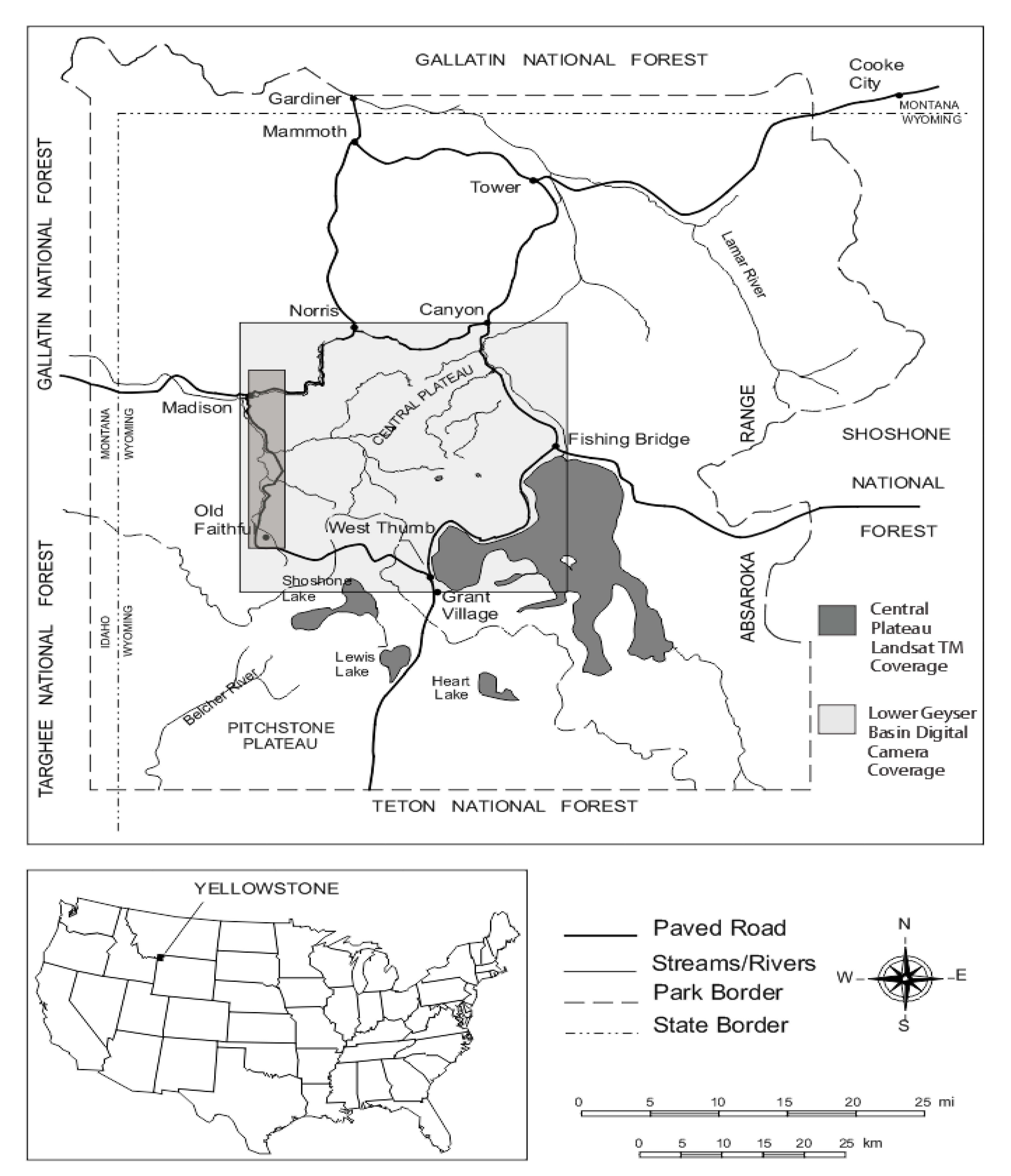
2.1. Study Area

Yellowstone National Park, the oldest park in the United States, is located in the northwest corner of Wyoming and adjacent to Montana and Idaho. The park and encompasses about 9000 km² of mostly high, forested plateau (Figure 1). The vegetation of the plateau is controlled mainly by elevation, with moisture generally increasing with elevation, and the geological substrate likewise related to the soil formation [1]. The coniferous forest canopy of Yellowstone is dominated by lodgepole pine (Pinus contorta var. latifolia). However, older stands, approximately 250 to 350 years old are comprised mostly of subalpine fir (Abies lasiocarpa) and Engelmann spruce (Picea engelmanni). Douglas fir (Pseudosuga menziesii) is also present in the region. Historically, fire was a common natural disturbance in the region, most recently as the dramatic fires of 1988, which burned almost 45% of the park [1]; fires of such scale occurring in the past, most recently in the early 1700s [43]. This preliminary study was limited to the eastern part of the Central Plateau of Yellowstone National Park, specifically, the Lower Geyser Basin, due to the spatial extent of the hyperspatial digital imagery. The post-burn lodgepole pine regenerating sites vary greatly in seedling density from a few trees per hectare to thousands seedlings per hectare. As the fire burned mainly in old growth there are large fallen logs in the understory and some standing logs.

Figure 1. Study area, a footprint of a Landsat TM scene is show for reference.

Figure 1. Study area, a footprint of a Landsat TM scene is show for reference.

2.2. Field Data

We utilized a fully random sampling method to collect field data in the postfire sites during the summers of 2001 and 2002 in the Lower Geyser Basin on the western periphery of the Yellowstone Central Plateau. We chose a fixed plot method of ground sampling for collection of field estimates of seedling densities. The plots were located well within homogenous areas of the regenerating burns, by choosing plots away from the edges of the stands. We counted all seedlings in all, 20 m by 20 m plots. Other data reported included the basal area of the dead standing wood in the plots. In total 62 field plots were collected coincided with coverage of the hyperspatial imagery described in the next section. At each plot a stem map was surveyed and generated using a 1 by 1 m grid, measuring tape and a compass. The plots were located using a differential GPS. Field data was only acquired for map validation and was not used in the generation of the classifications.

2.3. Remotely Sensed Data

A customized DuncanTech MS3100 multispectral digital camera owned by the Kansas Applied Remote Sensing (KARS) Program was used to collect 40 cm ground space distance imagery over the Lower Geyser Basin sites on the western periphery of the Yellowstone Central Plateau, between July 18th and 20th, 2001The image area for each frame was 1392 × 1040 pixels or approximately 0.4 by 0.5-km on the ground. We used a progressive scan to acquire clear images of mobile targets at frame rates of up to 7.5 fps. The Lower Geyser Basin overflight required 15 flight lines that were 15 km in length. Three spectral bands were collected: blue (450–520 nm), red (630–690 nm) and near-infrared (760–900 nm). Features such as roads and field-surveyed targets were used to georectify the imagery and individual scenes were mosaiced to produce continuous coverage of areas in the Lower Geyser Basin. The continuous mosaic was then orthorectified with a 10-meter resolution digital elevation model, the root mean square value (RMS) for the project area was: 0.27 meters. Additional imagery available for reference purposes included black and white digital orthophotograph quarter quadrangle images and Advanced Spaceborne Thermal Emission and Reflection Radiometer scenes. The atmospheric conditions during the data acquisition flights were optimal and ground spectra collected during the flight indicated minimal atmospheric disturbance in the visible portion of the spectrum; the data were not atmospherically.

We used the near-infrared band of the digital sensor to derive coarse and fine SOIT fields. This band was selected to better distinguish between live and dead tree crowns, as well as help in the separation between understory grass and the mainly coniferous crowns. There are many possible texture measures that can be extracted from the spatial co-occurrence matrix [14], the original texture developers, present as many as fourteen different measures. Many of these measures are redundant and capture similar concepts [22]. The contrast SOIT was applied in this project as it has been shown to be useful in forestry applications by others [23]. We compute this mean contrast texture field using the gray level co-occurrence matrix and the following equation:

(1)

where: P(i,j) = the spatial co-occurrence matrix element (line, row).

The window size of the texture measure, which is the extent of pixels used to quantify texture, is known to influence the results of texture analysis and is a multiscale phenomenon [24]. In this project, two texture window sizes were used, a 3 by 3-fine window and a 21 by 21-coarse window. The derived mean contrast texture image created by applying Equation 1 to a 3 by 3-pixel window was visually interpreted to capture the seedling crowns, the imagery is shown in Figure 2. We chose the window size based on previous work with texture [40,44]. The texture field created using a coarser image window produced imagery that summarized stand types, and visually showed some relationship to stand density. Texture was imported as an image band because the textures available in Trimble’s eCognition computes texture as an average for the segmented objects; thus, texture cannot be used until image segmentation has already been performed. This is image–based texture based on the gray level co-occurrence matrices which hybridizes the spatial and spectral properties of imagery in the texture measure; it has been show to improve classification results in work with hyperspatial imagery [39,45]. The texture calculated by eCognition is segment based texture not image-based texture, it has not been compared to results based on image derived texture. In this approach, we used SOIT calculated using ENVI software, to influence the boundaries of objects obtained through image segmentation. Furthermore, the approach in this project differs from the usage of the SOIT offered by eCognition, because texture fields of different window sizes can be implemented, producing fine and coarse image texture fields.

Figure 2. Example of false color composite image and fine image texture used to highlight the seedling crowns in the near-infrared band of the hyperspatial multispectral imagery.

Figure 2. Example of false color composite image and fine image texture used to highlight the seedling crowns in the near-infrared band of the hyperspatial multispectral imagery.

2.4. Object-Based Image Analysis (OBIA) Approach

We developed a semi-automated hierarchical methodology to facilitate using the same protocol to classify other subsets of the imagery using a batch process.

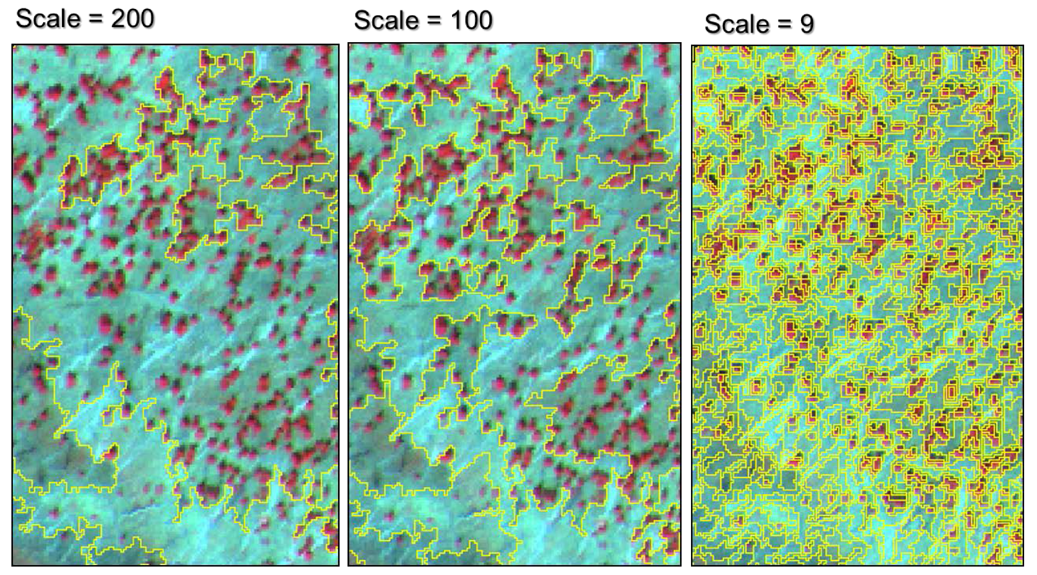
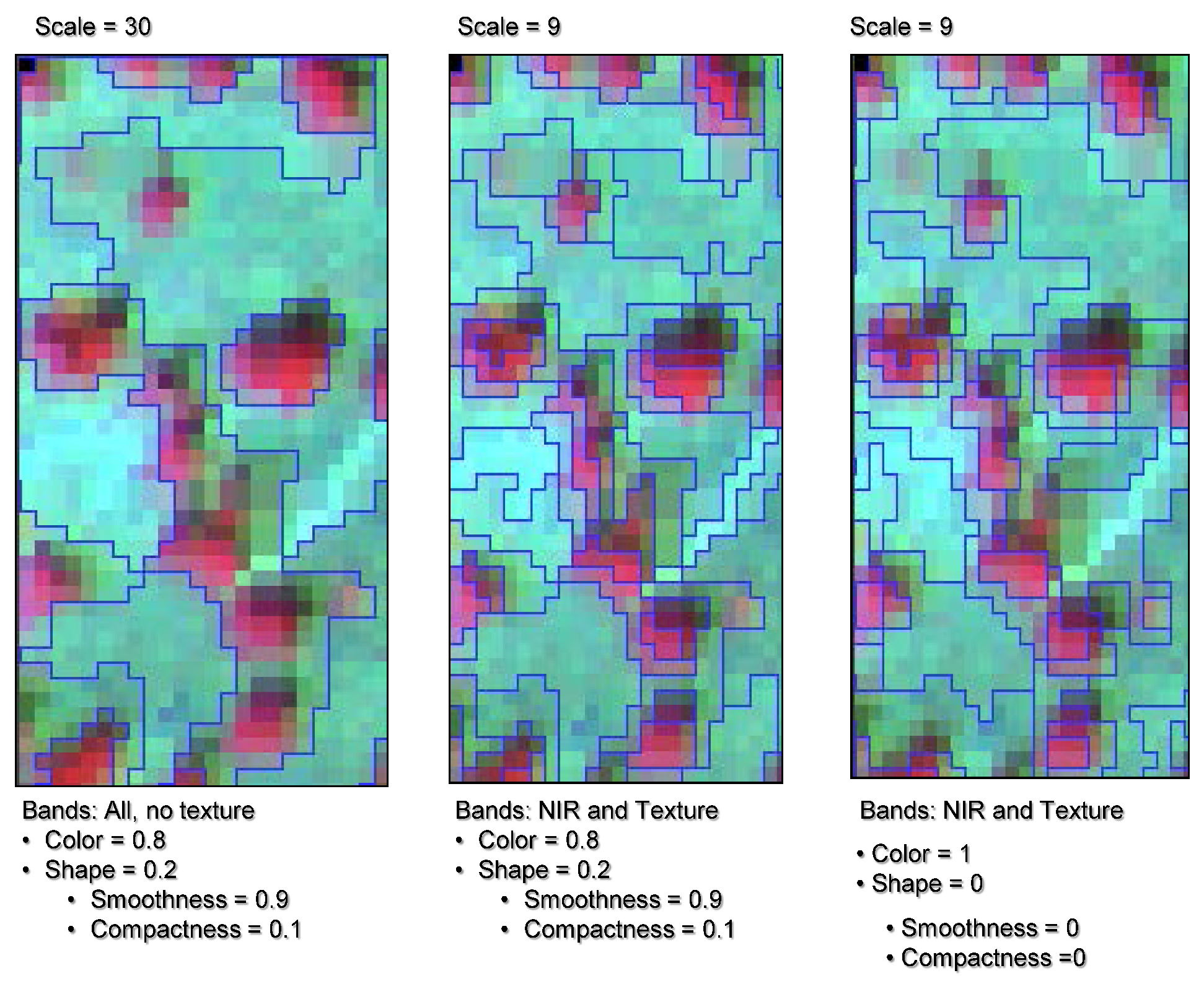
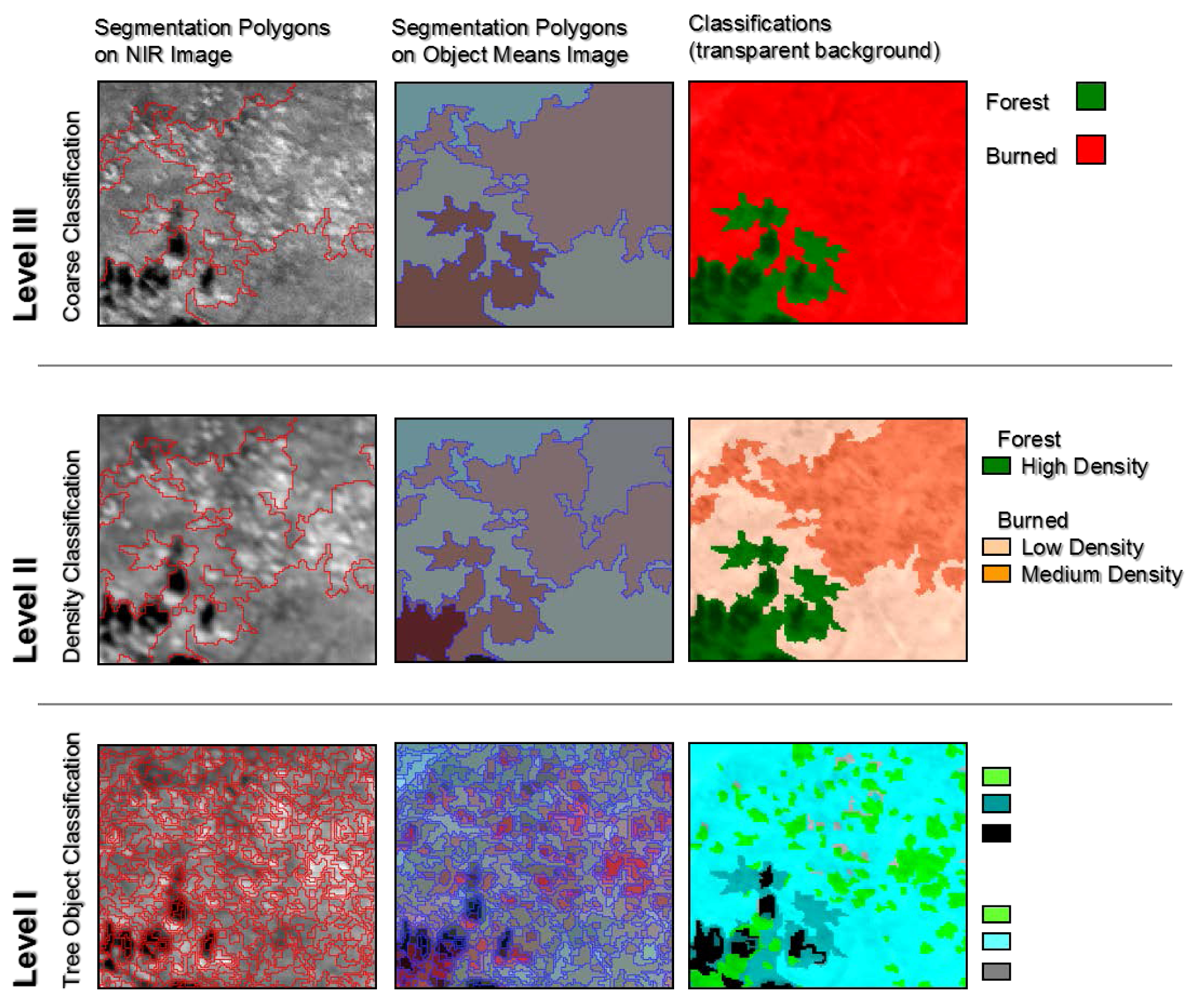
2.4.1. Hierarchical Segmentation

In the hierarchical segmentation approach, we used Trimble eCognition to identify image objects representing three hierarchical levels required for classification. The segmentation at Level III identified objects that can be easily grouped to coarse classification structures, consisting: water, clearings, forest, roads and clouds. We used segmentation Level II to identify specific areas of detail within the parent objects, such as different seedling density classes within the burn class. We grouped the seedling densities to classes similar to work by Turner et al. [46]; where low density had less than 1000 seedlings per hectare, medium density had over 1000–50,000 seedlings per hectare and high density had over 100,000 seedlings per hectare. Segmentation Level I aimed at producing objects that characterized tree crowns and other stand characteristics including shadows and understory.

For the hierarchical segmentation at the three different levels, various parameters required specification of spectral bands for the segmentation. Visual interpretation of the imagery demonstrated that the near-infrared band was far superior at identifying tree crowns at Level I, this is due to the high contrast between the crowns and the surrounding background matrix material comprised of other vegetation such as dried grass. However, all three spectral bands were useful at identifying boundaries at Levels II and III. Thus, bands were weighted according to their importance such that the near-infrared band had a weight of one assigned, and the red and blue bands had weights of 0.5 assigned. The textural bands were weighted at 0.5 in the Level I segmentation and only used at this Level I. The 32-bit texture image allowed for a higher gradient of gray level values to be calculated. This made the texture band as important as the other weighted band in the Level I segmentation. The rationale for the application of texture at only the Level I segmentation is explained in the Results section.

We performed scale parameter (SP) selection as well as decisions based on how much weight to assign to color, shape, smoothness and compactness visually; we use Figure 3 to demonstrate the role of some of these parameters. Note that the selection of the parameter values influences how well the segments match interpretable image objects such as tree crowns. The SP values at the three segmentation levels are reported in Table 1, along with resulting object characteristics. As expected, when using a low SP the number of objects dramatically increases, reducing the average objects size. This greatly contributed to an increase in processing time.

Table 1. Scale parameters at the three segmentation levels and associated object characteristics.

Segmentation Level	Scale Parameter	Number of Objects	Average Object Size (m2)	Average Neighborhood (segments)
III	200	84	160,000	4.4
II	100	317	4,245	4.71
I	9	39,665	33.92	5.36

Table 1. Scale parameters at the three segmentation levels and associated object characteristics.

Segmentation Level	Scale Parameter	Number of Objects	Average Object Size (m2)	Average Neighborhood (segments)
III	200	84	160,000	4.4
II	100	317	4,245	4.71
I	9	39,665	33.92	5.36

Figure 3. Scale, color, shape, smoothness and compactness parameters used for selecting the most optimal segmentation. A scale parameter of 30 generates smallest segments of about 5 m in width and can capture large crowns and sub-stand characteristics, in comparison a scale parameter of 9 generates smallest segments of about 1m in width and can segments trees to sub components such as crowns and shadows. The higher the scale parameter the more general the segments are, thus, in this resolution imagery a scale parameter of 100 captures general stand types and a scale parameter of 200 can capture general landscape classes.

Figure 3. Scale, color, shape, smoothness and compactness parameters used for selecting the most optimal segmentation. A scale parameter of 30 generates smallest segments of about 5 m in width and can capture large crowns and sub-stand characteristics, in comparison a scale parameter of 9 generates smallest segments of about 1m in width and can segments trees to sub components such as crowns and shadows. The higher the scale parameter the more general the segments are, thus, in this resolution imagery a scale parameter of 100 captures general stand types and a scale parameter of 200 can capture general landscape classes.

The shape parameter also required careful consideration. A high degree of shape criterion works at the cost of spectral homogeneity [19]. However, the spectral information is, at the end, the primary information contained in image data. Using too high of a shape criterion can therefore reduce the quality of segmentation results. We suggest that removing a shape criterion from the segmentation, a higher scale parameter can be implemented without losing the object definition at the Level I segmentation, thus reducing processing time and CPU usage, and helping in within crown characterization. This is demonstrated by comparing the images in Figure 3. Moreover, at this hyperspatial per-pixel resolution, low scale parameters such as 9 capture within tree variability, medium parameters such as 100 capture stand characteristics and high parameters such as 200 capture landscape complexity, and this is demonstrated in Figure 4.

Figure 4. Examples of different scale parameters and impacts on the segmentation.

Figure 4. Examples of different scale parameters and impacts on the segmentation.

In addition to the above parameters we used the Brightness, Blue mean value, Red Mean value, Near-infrared Mean value, Area, Length of object border, Proximity (distance) to other classes, and perimeter to area ratio. Selection of these parameters was decided based on previous research with hyperspatial aerial photography and visual interpretations of outputs through a trail-and-error approach [47].

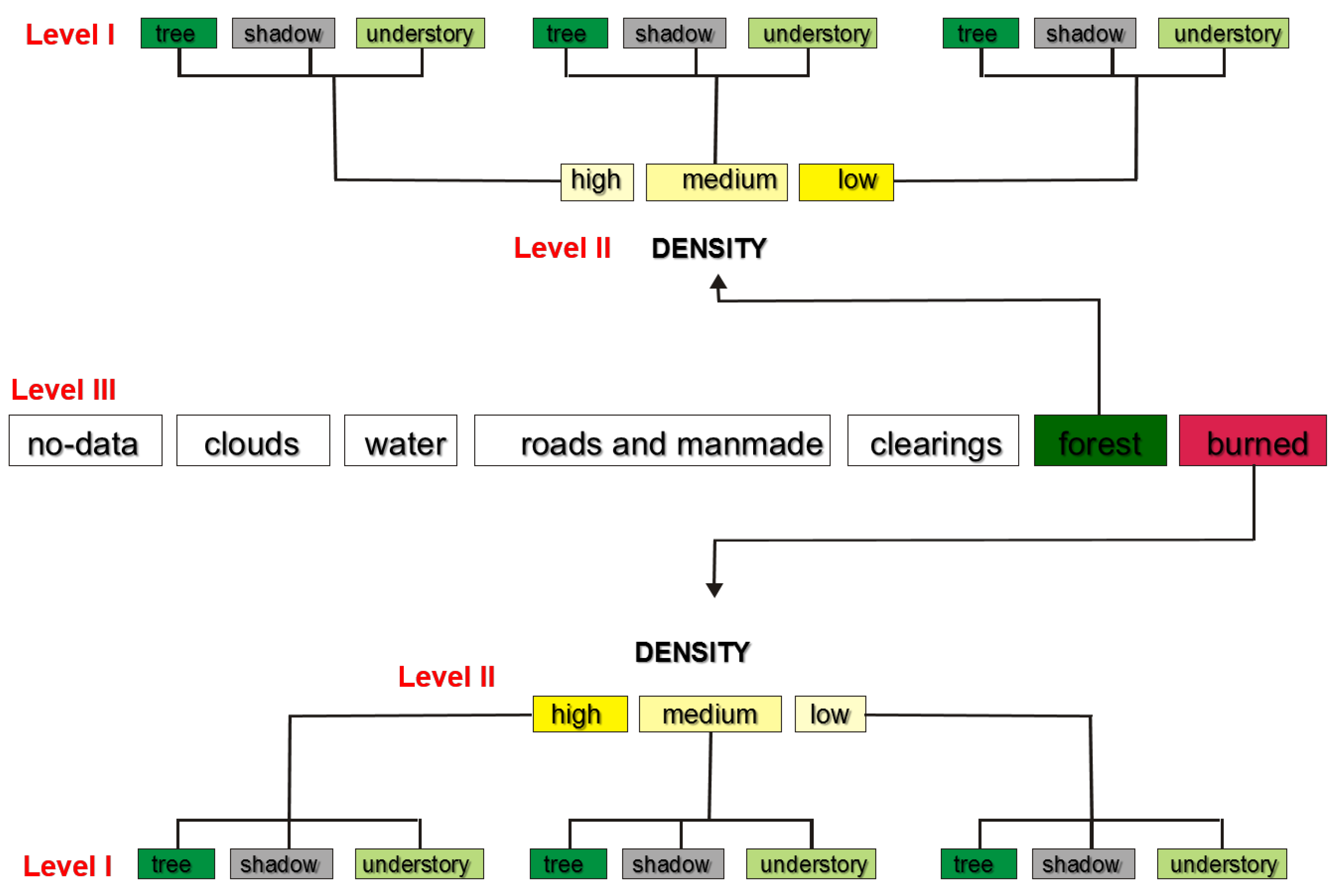
2.4.2. Hierarchical classification

Three hierarchical levels of classification were also developed through a supervised classification approach where a quarter of the field plots (Level II) and photo interpreted sites (Level I and Level III) were used for the training of the classifier and the remaining samples were used for validation. The photo interpreted points for Level I and Level III used for training the classifier were interpreted by a different person then the randomly selected points used to test the classifier. Both interpreters were experience at photo interpretation in forestry applications, thus, we assume high confidence in the photo interpretation as others have done [48].

Level III focused on a coarse classification of the imagery to general landuse/landcover (LULC) classes. Such level of information can often be obtained from LULC maps or GIS data, but was not available for this project. Level II, the seedling density classification, can often be obtained from forest inventory GIS coverages, but these are not necessarily accurate and are very often out of date due to the long time required to acquire traditional manual forest inventory classification. Finally, the Level I classification concentrated on tree and stand objects. It is only with automated, or semi-automated digital data approaches that such highly detailed types of information can be feasibly extracted for entire landscapes.

The highest classification level, Level III consisted of general classes: forest, burn, clearings, roads and manmade, water, and clouds. This first general classification allowed for extraction of two specific classes of interest in forest characterization, the burn and the mature forest class; all other classes were ignored in further hierarchies. Subsequently, these two classes were classified to three forest and seedling density classes specific to the owner class, at the Level II classification. This is particularly important because the seedlings and mature trees are quite different in size that their densities need to be extracted independently. Lastly, tree crowns, shadows and understory were extracted at the finest Level I classification. The hierarchical classification approach is summarized in Figure 5.

Figure 5. Three level hierarchical classification scheme.

Figure 5. Three level hierarchical classification scheme.

The groups of classes were formed for the three classification levels. At the highest and coarsest Level III of the classification, the classes were identified independently of any other Level and the Level III segmentation was used to identify polygons representing the seven classes. Nearest neighbor classifier applied the information contained for each class including the values in the three spectral bands and standard deviation of these bands. The classification was limited to the Level III segmentation. The subsequent Level II classification inherited all class characteristics from Level III classes, but only for classes such as water or clouds. The mature forest and burn classes inherited the spectral characteristics from their parent (Level III) classes, but were further defined by the implementation of fine texture in their feature definition so that the seedling density classes could be established. The coarse image texture was experimented with but based on visual interpretation the output was not favorable. The convergence of texture values at 21 by 21 window in Figure 6. This is likely due to the within crown characteristic being captured by the fine image texture at the particular pixel resolution, these are a detail level above of what the Level II classes were meant to capture. The Level II classification was limited to polygons derived from the Level II segmentation. Level I classification, still used the inheritance features for the water and cloud classes, but the three new classes of crown, shadow and understory were defined by their spectral and textural characteristics. Few of the shape descriptors were used to define the crown class. Relations to super-objects from the Level III and Level II classifications were also implemented. The Level I classification was limited to polygons derived from the Level I segmentation.

Figure 6. Texture results for varying window sized of image texture.

Figure 6. Texture results for varying window sized of image texture.

2.5. Classification Assessment

Based on areas visited in the field, polygons of known forest densities and class types were located in the three levels of segmentation and used to visually assess class separability based on various feature spaces such as the spectral and textural bands. Inherent to the eCognitions’ fuzzy classification concept, an image object has a membership degree to more than one class. With the classification stability tool, the differences in degrees of membership between the best and the second best class assignments of each object, which can give evidence of the ambiguity of an object’s classification, were explored. The graphical output of classification stability can be visually assessed as values are displayed for each image object in a range from dark green (1.0, non-ambiguous) to red (0.0, ambiguous). Classification accuracy matrices [25] for the three hierarchical classification levels, based on the manually selected assessment polygons, were produced and summarized. A confusion matrix for each hierarchical level was also developed [49], using the 62 field validated sites and additional imagery interpreted observations. For Level III, the 62 burned field validated sites were used as well as visually interpreted: 20 forest sites, 10 clearings, 5 roads, 5 water. In Level III only the Clearing, Forest and Burned sites were used in the generation of the final confusion matrix so as not to inflate the accuracies with easy to map classes such as water and roads which did not show issues of confusion upon visual assessment [49]. At Level II the confusion matrix was generated using the 62 field sites stratified to high, medium and low densities based on the field density tallies, the high density class had 18 observations, medium density class has 22 observations and low density class had 22 observations. Finally, for the confusion matrix at Level I, a visual interpretation identified 600 points evenly divided between crown, shadow and understory.

3. Results and Discussion

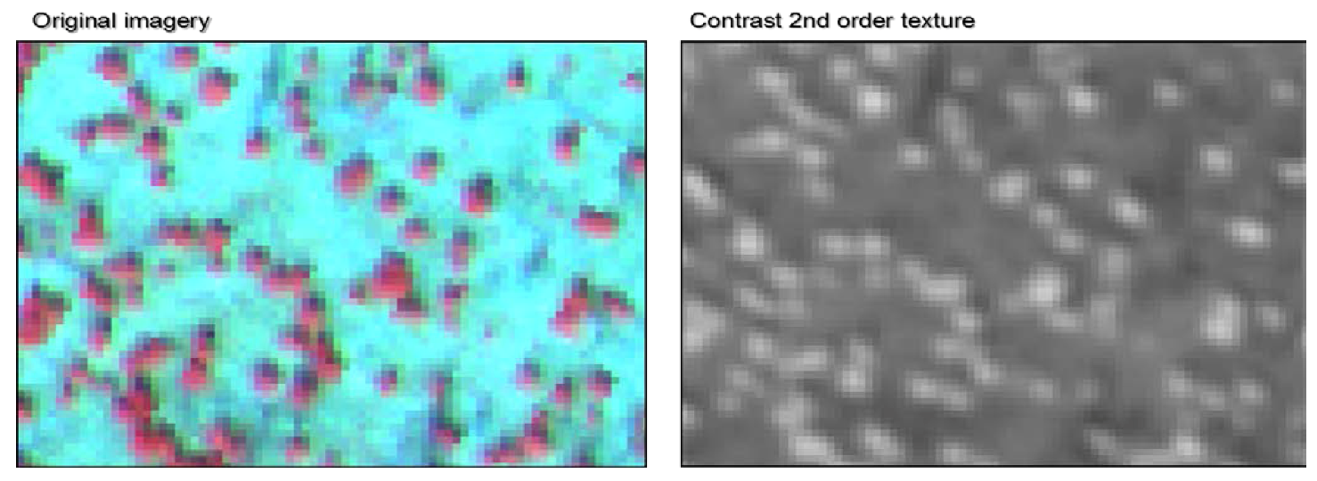
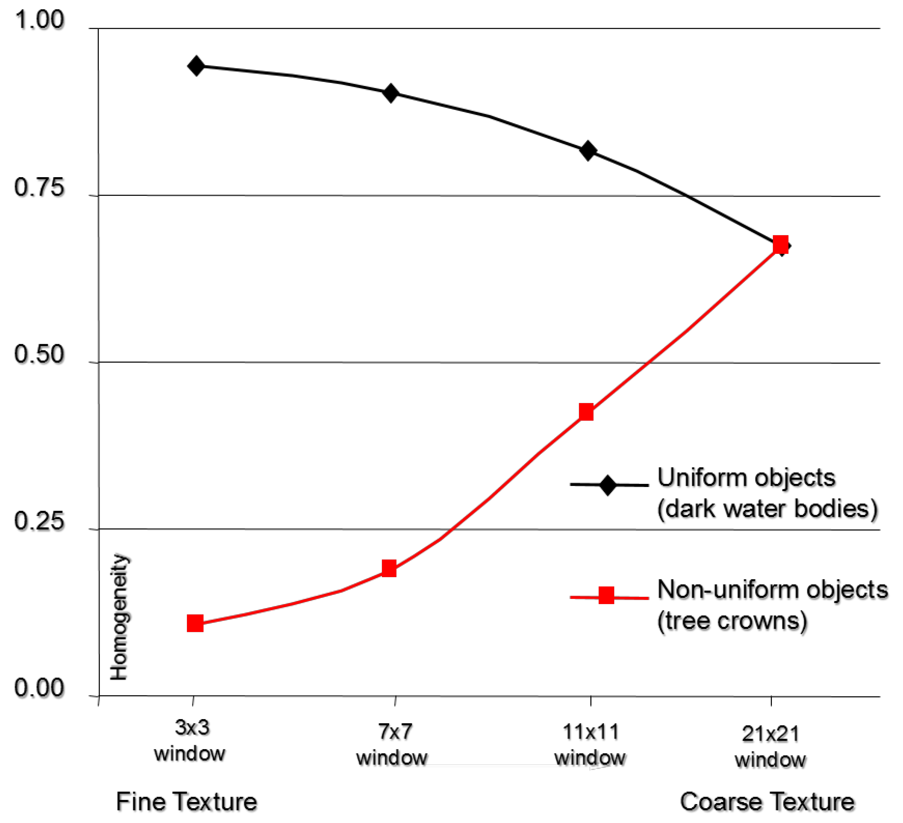
3.1. Application of Image Texture

Investigation of fine and coarse image texture in the segmentation and the hierarchical classification procedures determined the fine texture is useful in small-scale segmentation, because tree crowns and shadows can be better delineated in the fine texture imagery than in the original near-infrared band of the imagery. However, coarse texture is not applicable in large-scale (SP over 30) segmentation. This is due to the boundary averaging resulting from larger window sizes used to calculate the coarse texture. For example, areas with strong boundaries expressed by high or low digital number (DN) values cause a ‘smudging’ effect where the boundary DN values are averaged. Thus, areas that are highly uniform are susceptible to increases in texture as the scale of observation decreases (going from a large to small window size). Non-uniform landscape areas, for example: seedling forest stands, decrease in texture values including mean contrast as the scale of observation increases. We demonstrate this phenomenon in values observed in Table 2. In the Level II hierarchical classification the coarse texture can be used as one of the features that describe a particular class, and was found to be particularly successful in relating seedling densities.

Table 2. Change in texture of uniform and non-uniform objects at different scales of observation.

	Mean Contrast Texture
	Uniform object	Non-uniform object
	(i.e., image boundary)	(i.e., seedlings)
fine	0.9435	0.1090
	0.9050	0.1910
	0.8148	0.4211
coarse	0.6739	0.6725

Table 2. Change in texture of uniform and non-uniform objects at different scales of observation.

	Mean Contrast Texture
	Uniform object	Non-uniform object
	(i.e., image boundary)	(i.e., seedlings)
fine	0.9435	0.1090
	0.9050	0.1910
	0.8148	0.4211
coarse	0.6739	0.6725

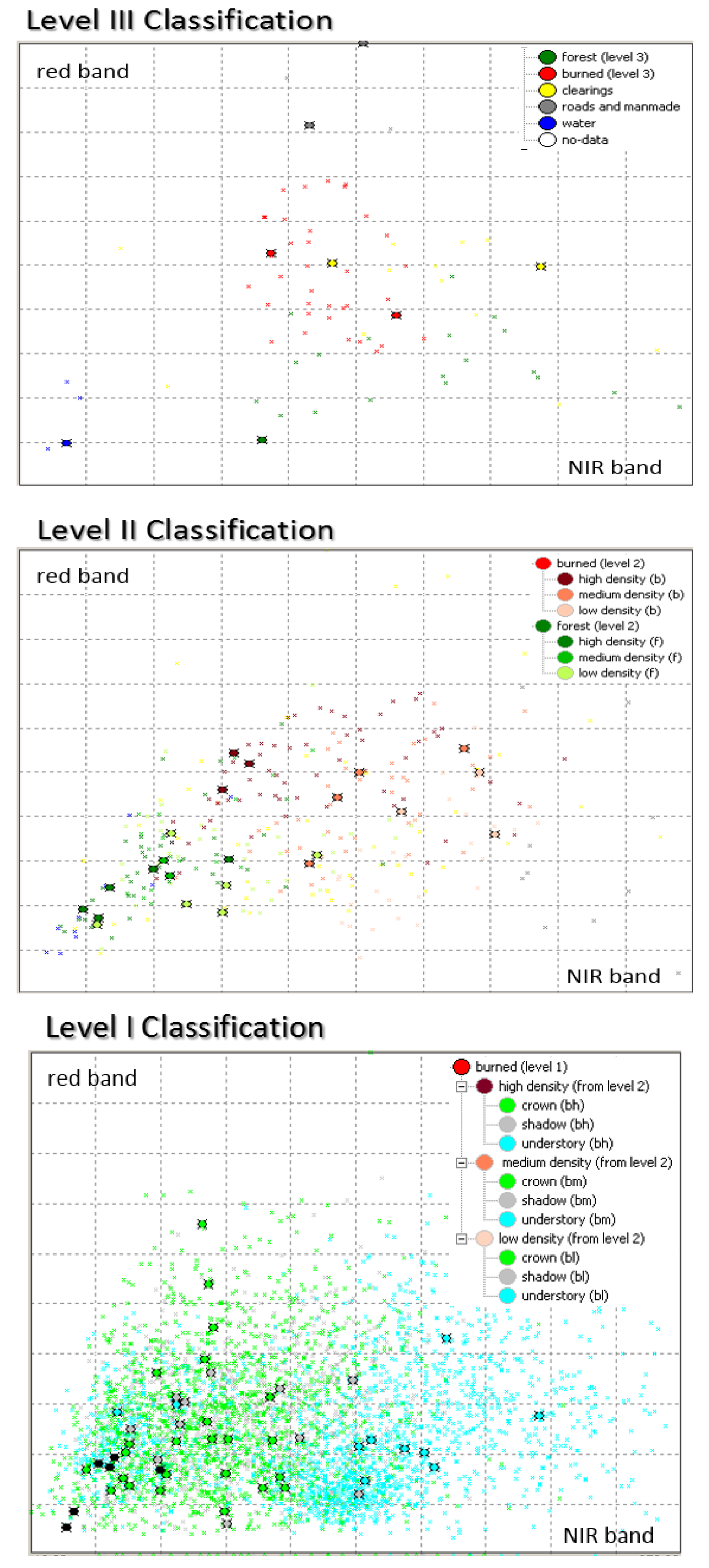
3.2. Hierarchical Classification

In Figure 7a small area of the classified imagery is shown at the three hierarchical classification levels. The polygons resulting from the three levels of segmentations are delineated and the mean average band values for each of the polygons are represented in the false color composite images.

Figure 7. Close-up of the classified imagery at the three hierarchical levels.

Figure 7. Close-up of the classified imagery at the three hierarchical levels.

It is easy to observe in Figure 4 that the level of detail captured by each of the hierarchical segmentations increases, where a segmentation with an SP of 200 captures broad stand types, segmentation with a SP of 9 captures within seedling crown detail such as shadow, lit ground and surrounding understory. However, at Level I it was anticipated that the objects would clearly represented individual tree crowns, but due to the small size of the seedling, the 40 cm per pixel imagery is not fine enough in resolution to capture such detail. Thus, individual seedling crowns are not always captured by the objects classified at Level I, what is captured are the areas of tree crowns as opposed to the understory and areas covered by shadow. Although methodologies using individual stem counts [11], cannot be applied to determine seedling densities per polygon (Level II polygons), the average area of tree crowns per polygon can be used as a method of estimating seedling density. Interpreting this type of information manually takes many hours and requires very skilled photo interpreters. The same interpreters can apply their skill to the semi-automated methodology presented here and achieve forest inventory characteristics on a timelier basis. In comparison, the crowns of the larger trees can be identified as individual crowns and quantified on a stem-by-stem basis. The initial visual interpretation of these results suggests that another segmentation level, specifically aimed at identifying large tree crowns could be implemented. The SP of 9 for segmentation of the seedling crowns is too fine for the mature forest crowns, an increase in processing speed and a better defined crown could be achieved with a slightly larger SP (i.e., 30).

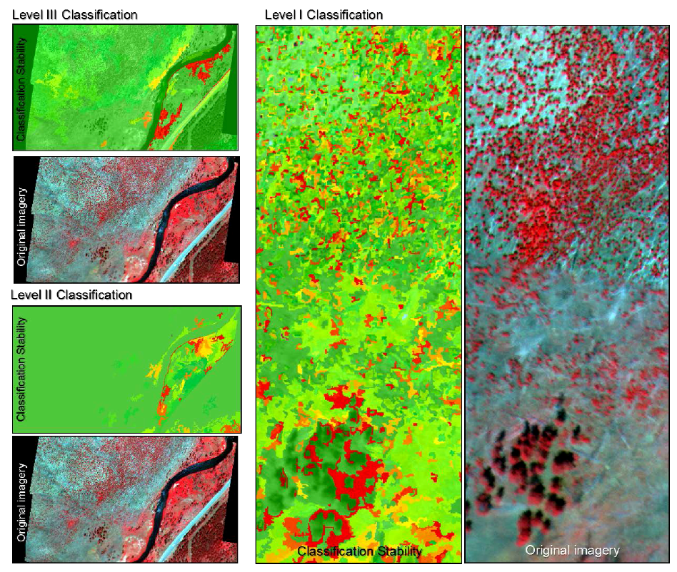
3.3. Class Separability and Classification Stability Assessments

Figure 8 represents the spectral (near infrared and red bands) ‘feature space’ for classified and reference objects for the three hierarchical classification levels. Visually, it can be determined that the clearings and the burn class, in the Level III classification, show some overlap along the mixed-pixel edge of the classes. One approach to control for this would be to use a GIS burn perimeter, if one is available. In Level II classification, the low-density mature forest class and medium-density burn class occupy similar areas in the two dimensional feature space. In Level I classification the greatest overlap between classes occurs.

Figure 8. Feature space plots (NIR and red bands) for assessment sites at the three hierarchical levels of classification.

Figure 8. Feature space plots (NIR and red bands) for assessment sites at the three hierarchical levels of classification.

We evaluate classification accuracies and class assignments through the confusion matrices (Table 3, Table 4 and Table 5) and also show the feature space plots in Figure 8. Table 3-Level III classification had an average accuracy of 89.1%, when standardized 77.7%. Confusion occurred between the clearing and burn class, with almost equal errors of omission and commission for each class. The other LULC classes were removed from the confusion matrix calculations because these were not related to this work focusing on forestry applications and not general LULC classification. One way to enhance this classification would be to use an object association approach, especially for large clearings that tend to occur next to roads or water. Table 4-Level II classification accuracy on average reached 85.4% and the standardized accuracy was 78.2%. Although the signatures of the low-density mature forest class and medium-density burn class occupy similar areas in the two dimensional feature space, this is not where the errors in the classification occur, as the Table 3-Level III classification easily distinguishes between these classes and the class information in fully inherited by the Table 4-Level II classification. Most discrepancies occurred between the medium and low-density classes, in both the mature forest and the burn class. Lastly, the Table 5-Level I classification average accuracy was 78.8%, standardized to 68.2%. There were many errors of omission and commission between the classes, and minimal errors which were in inherited from the Table 3-Level III and Table 4-Level II due to the inheritance functions. Additional spectral information in SWIR-bands, including bands 5 and 7 of Landsat, may provide improvements, as the structural changes to the stands post-fire result in higher SWIR-bands reflectance. This is precisely why this spectral region is used in characterizing burn classes by researchers utilizing Landsat [14,30,50] however, this spectral range was not available from our sensor. Another issue in accuracy, the assessment of the segments (tree crowns), was not investigated in this work because only a limited number of methods for this validation have been developed and are not yet mature [51].

Table 3. Classification accuracies summarized in a confusion matrix for each hierarchical level. Level III: Validation of LULC Forest and Burned Classes Only.

		Reference Data
	Class	Forest	Burned	Clearing		Total	Producer’s Accuracy
Classification Data	Forest	17	3	0		20	85.0%
	Burned	3	57	2		62	91.9%
	Clearing	0	2	8		10	80.0%
	Total	20	62	10		92
	User’s Accuracy	85.0%	91.9%	80.0%
	Overall Accuracy	89.1%
	Khat	0.78

Table 3. Classification accuracies summarized in a confusion matrix for each hierarchical level. Level III: Validation of LULC Forest and Burned Classes Only.

		Reference Data
	Class	Forest	Burned	Clearing		Total	Producer’s Accuracy
Classification Data	Forest	17	3	0		20	85.0%
	Burned	3	57	2		62	91.9%
	Clearing	0	2	8		10	80.0%
	Total	20	62	10		92
	User’s Accuracy	85.0%	91.9%	80.0%
	Overall Accuracy	89.1%
	Khat	0.78

Table 4. Classification accuracies summarized in a confusion matrix for each hierarchical level. Level II: Validation of Seedling Densities.

		Reference Data
	Class	Low	Medium	High		Total	Producer’s Accuracy
Classification Data	Low	15	2	1		18	83.3%
	Medium	3	19	0		22	86.4%
	High	2	1	19		22	86.4%
	Total	20	22	20		62
	User’s Accuracy	75.0%	86.4%	95.0%
	Overall Accuracy	85.5%
	Khat	0.78

Table 4. Classification accuracies summarized in a confusion matrix for each hierarchical level. Level II: Validation of Seedling Densities.

		Reference Data
	Class	Low	Medium	High		Total	Producer’s Accuracy
Classification Data	Low	15	2	1		18	83.3%
	Medium	3	19	0		22	86.4%
	High	2	1	19		22	86.4%
	Total	20	22	20		62
	User’s Accuracy	75.0%	86.4%	95.0%
	Overall Accuracy	85.5%
	Khat	0.78

Table 5. Classification accuracies summarized in a confusion matrix for each hierarchical level. Level I: Validation of Objects (Shadow, Crown and Understory).

		Reference Data
	Class	Tree	Shadow	Understory		Total	Producer’s Accuracy
Classification Data	Tree	149	2	13		200	74.5%
	Shadow	39	149	12		200	74.5%
	Understory	12	13	175		200	87.5%
	Total	200	200	200		600
	User’s Accuracy	74.5%	74.5%	87.5%
	Overall Accuracy	78.8%
	Khat	0.68

Table 5. Classification accuracies summarized in a confusion matrix for each hierarchical level. Level I: Validation of Objects (Shadow, Crown and Understory).

		Reference Data
	Class	Tree	Shadow	Understory		Total	Producer’s Accuracy
Classification Data	Tree	149	2	13		200	74.5%
	Shadow	39	149	12		200	74.5%
	Understory	12	13	175		200	87.5%
	Total	200	200	200		600
	User’s Accuracy	74.5%	74.5%	87.5%
	Overall Accuracy	78.8%
	Khat	0.68

By visually evaluating the stability images produced with Trimble eCognition, objects with ambiguity values of 0.2 or less were displayed in red tones and easily pinpointed (Figure 9). These objects obtained a high degree of membership in more than one class. At the Table 3-Level III classification, the areas of poor stability occurred near the riverbanks. The approach of associating objects with their neighborhoods should advance the stability and accuracy of this classification by associating areas neighboring the water as clearings and not as low-density regenerating forest stands. The instability in the clearing areas near the river is propagated to the lower level of the hierarchical classification, suggesting that if the Table 3-Level III coarse classification can be enhanced then the Table 4-Level II classification would benefit as well. Spatial patterns and spatial associations are not inherent and rarely utilized in per pixel classification algorithm, this type of approach is only inherently available in an OBIA classification scheme. Finally, we observe by evaluating the Table 5-Level I stability image that the instability of this classification does not propagate down from the higher Table 3-Level III and Table 4-Level II classifications. Thus, the instability in this classification is independent of the inheritance of the classes. The areas of instability do not seem to have a strong spatial pattern to them, however, some trend perhaps associated with three size and densities should be further investigated.

Figure 9. Visual analysis of classification stability; stability scale is a color ramp where dark green is non-ambiguous (1) and red is absolutely ambiguous (0).

Figure 9. Visual analysis of classification stability; stability scale is a color ramp where dark green is non-ambiguous (1) and red is absolutely ambiguous (0).

4. Conclusions

Object-based image analysis (OBIA) of hyperspatial multispectral imagery is a unique approach to forest inventory characterization. The semi-automated approach utilizes the photo interpretation skills of the user, but due to the automation, it can greatly cut down on processing time compared to traditional manual methods. The method performs well in quantifying seedling density, although improvements could still be made. The SOIT performs well and can be utilized as a spatial component variable in OBIA segmentation or classification methodologies. The hierarchical approach developed here shows great potential for building complex conceptual relationship between image objects, which can greatly improve classification methods using only spectral per pixel signatures. When available, Level III classifications can be substituted by LULC maps and similarly, Level II classifications can be substituted by forest inventory maps, it is Level I classifications that are the most useful for refining and updating those inventories. Spatial and hierarchical associations are also a strength that this methodology utilizes and can be exploited with the substituted data types. Because the image resolution is not optimal for seedling crown identification, we conclude that developing relationships between forest inventory variables including crown diameter and height with image-derived parameters are not feasible for the seedling polygons, but can be feasible for the mature forest polygons. Climate change is impacting post-disturbance regeneration rates [52]. The method demonstrated here captures the spatial patterns of post-disturbance regeneration of forests, a basic knowledge parameters for adaptive management to landscape stewardship under climate change [53].

References

1. Romme, W.H.; Despain, D.G. On historical perspective fires of 1988 Yellowstone comparable. Perspective 2011, 39, 695–699. [Google Scholar]
2. Romme, W.H.; Boyce, M.S.; Gresswell, R.; Merrill, E.H.; Minshall, G.W.; Whitlock, C.; Turner, M.G. Twenty years after the 1988 Yellowstone Fires: Lessons about disturbance and ecosystems. Ecosystems 2011, 14, 1196–1215. [Google Scholar] [CrossRef]
3. Christensen, N.L.; Agee, J.K.; Brussard, P.F.; Hughes, J.; Dennis, H.; Minshall, G.W.; Peek, J.M.; Pyne, S.J.; Swanson, F.J.; Thomas, W.; Wells, S.; Williams, S.E.; Wright, H.A.; Knight, D.H.; Swanson, J.; Thomas, J.W.; Williams, S. The Yellowstone interpreting fires ecosystem responses and management implications. BioScience 1989, 39, 678–685. [Google Scholar] [CrossRef]
4. Moskal, L.M.; Dunbar, M.; Jakubauskas, M.E. Visualizing the forest: a forest inventory characterization in the Yellowstone National Park based on geostatistical models. In A Message From the Tatras: Geographical Information Systems & Remote Sensing in Mountain Environmental Research; Widacki, W., Bytnerowicz, A., Riebau, A., Eds.; Institute of Geography & Spatial Management, Jagiellonian University: Krakow, Poland, 2004; pp. 219–232. [Google Scholar]
5. Turner, M.G.; Romme, W.H.; Tinker, D.B. Surprises and lessons from the 1988 Yellowstone fires In a nutshell. Front. Ecol. Environ. 2003, 1, 351–358. [Google Scholar] [CrossRef]
6. Merrill, E.H.; Bramble-brodahl, M.K.; Marrs, R.W.; Boyce, M.S. Estimation of green herbaceous phytomass from Landsat MSS data in Yellowstone National Park. J. Range Manag. 1993, 46, 151–157. [Google Scholar] [CrossRef]
7. Wambolt, C.L.; Rens, R.J. Elk and fire impacts on mountain big sagebrush range in Yellowstone. Nat. Resour. Environ. Issues. 2011, 16, 1–6. [Google Scholar]
8. Forester, J.D.; Anderson, D.P.; Turner, M.G. Do high-density patches of coarse wood and regenerating saplings create browsing refugia for aspen (Populus tremuloides Michx.) in Yellowstone National Park (USA)? For. Ecol. Manag. 2007, 253, 211–219. [Google Scholar] [CrossRef]
9. Wulder, M. Optical remote-sensing techniques for the assessment of forest inventory and biophysical parameters. Prog. Phys. Geogr. 1998, 22, 449–476. [Google Scholar]
10. Wang, J.; Sammis, T.W.; Gutschick, V.P.; Gebremichael, M.; Dennis, S.O.; Harrison, R.E. Review of satellite remote sensing use in forest health studies. Open Geogr. J. 2010, 3, 28–42. [Google Scholar] [CrossRef]
11. Mumby, P.J.; Green, E.P.; Edwards, A.J.; Clark, C.D. The cost-effectiveness of remote sensing for tropical coastal resources assessment and management. J. Environ. Manag. 1999, 55, 157–166. [Google Scholar] [CrossRef]
12. Smith, M.O.; Ustin, S.L.; Adams, J.B.; Gillespie, A.R. Vegetation in deserts: I. A regional measure of abundance from multispectral images. Science 1990, 26, 1–26. [Google Scholar]
13. Hyyppa, H.; Inkinen, M.; Engdahl, M. Accuracy comparison of various remote sensing data sources in the retrieval of forest stand attributes. Science 2000, 128, 109–120. [Google Scholar]
14. Miller, J.D.; Yool, S.R. Mapping forest post-fire canopy consumption in several overstory types using multi-temporal Landsat TM and ETM data. Remote Sens. Environ. 2002, 82, 481–496. [Google Scholar] [CrossRef]
15. Kashian, D.M.; Tinker, D.B.; Turner, M.G.; Scarpace, F.L. Spatial heterogeneity of lodgepole pine sapling densities following the 1988 fires in Yellowstone National Park, Wyoming , USA. Can. J. For. Res. 2004, 34, 2263–2276. [Google Scholar] [CrossRef]
16. Chambers, J.Q.; Asner, G.P.; Morton, D.C.; Anderson, L.O.; Saatchi, S.S.; Espírito-Santo, F.D.B.; Palace, M.; Souza, C. Regional ecosystem structure and function: ecological insights from remote sensing of tropical forests. Trends Ecol. Evol. 2007, 22, 414–423. [Google Scholar] [CrossRef]
17. Moskal, L.M.; Styers, D.M.; Halabisky, M. Monitoring urban tree cover using object-based image analysis and public domain remotely sensed data. Remote Sens. 2011, 3, 2243–2262. [Google Scholar] [CrossRef]
18. Platt, R.V.; Rapoza, L. An evaluation of an object-oriented paradigm for land use/land cover classification. Prof. Geogr. 2008, 60, 87–100. [Google Scholar] [CrossRef]
19. Blaschke, T. Object based image analysis for remote sensing. ISPRS J. Photogramm. Remote Sens. 2010, 65, 2–16. [Google Scholar] [CrossRef]
20. Townshend, J.R.G.; Huang, C.; Kalluri, S.N.V.; Defries, R.S.; Liang, S.; Yang, K. Beware of per-pixel characterization of land cover. Intern. J. Remote Sens. 2000, 21, 839–843. [Google Scholar] [CrossRef]
21. Myint, S.W.; Gober, P.; Brazel, A.; Grossman-Clarke, S.; Weng, Q. Per-pixel vs. object-based classification of urban land cover extraction using high spatial resolution imagery. Remote Sens. Environ. 2011, 115, 1145–1161. [Google Scholar] [CrossRef]
22. Cleve, C.; Kelly, M.; Kearns, F.; Mortiz, M. Classification of the wildland–urban interface: A comparison of pixel- and object-based classifications using high-resolution aerial photography. Comput. Environ. Urban Syst. 2008, 32, 317–326. [Google Scholar] [CrossRef]
23. Blaschke, T. Object based image analysis for remote sensing. ISPRS J. Photogramm. Remote Sens. 2010, 65, 2–16. [Google Scholar] [CrossRef]
24. Newman, M.E.; McLaren, K.P.; Wilson, B.S. Comparing the effects of classification techniques on landscape-level assessments: pixel-based versus object-based classification. Intern. J. Remote Sens. 2011, 32, 4055–4073. [Google Scholar] [CrossRef]
25. Franks, S. Monitoring forest regrowth following large scale fire using satellite data-A case study of Yellowstone National Park, USA. Eur. J. Remote Sens. 2013, 46, 551–569. [Google Scholar] [CrossRef]
26. Huang, S.; Crabtree, R.L.; Potter, C.; Gross, P. Estimating the quantity and quality of coarse woody debris in Yellowstone post-fire forest ecosystem from fusion of SAR and optical data. Remote Sens. Environ. 2009, 113, 1926–1938. [Google Scholar] [CrossRef]
27. Fu, G.; Zhao, H.; Li, C.; Shi, L. Segmentation for high-resolution optical remote sensing imagery using improved quadtree and region adjacency graph technique. Remote Sens. 2013, 5, 3259–3279. [Google Scholar] [CrossRef]
28. Polychronaki, A.; Gitas, I.Z. Burned area mapping in greece using spot-4 hrvir images and object-based image analysis. Remote Sens. 2012, 4, 424–438. [Google Scholar] [CrossRef]
29. Mitri, G.H.; Gitas, I.Z. Mapping the severity of fire using object-based classification of IKONOS imagery. Intern. J. Wildland Fire 2008, 17, 431–442. [Google Scholar] [CrossRef]
30. Potter, C.; Li, S.; Huang, S.; Crabtree, R.L. Analysis of sapling density regeneration in Yellowstone National Park with hyperspectral remote sensing data. Remote Sens. Environ. 2012, 121, 61–68. [Google Scholar] [CrossRef]
31. Mitri, G.H.; Gitas, I.Z. Mapping post-fire forest regeneration and vegetation recovery using a combination of very high spatial resolution and hyperspectral satellite imagery. Intern. J. Appl. Earth Observ. Geoinform. 2013, 20, 60–66. [Google Scholar] [CrossRef]
32. Haralick, R.M.; Shanmugam, K. Textural Features for Image Classification. IEEE Trans. Syst. Man Cybern. 1973, 3, 610–621. [Google Scholar] [CrossRef]
33. Irons, J.R.; Petersen, G.W. Texture transforms of remote sensing data. Remote Sens. Environ. 1981, 11, 359–370. [Google Scholar] [CrossRef]
34. Weszka, J.S.; Dyer, C.R.; Rosenfeld, A. A comparative study of texture measures for terrain classification. Comp. General Pharm. 1976, I, 41–46. [Google Scholar]
35. Carr, J.R.; de Miranda, F.P. The semivariogram in comparison to the co-occurrence matrix for classification of image texture. IEEE Trans. Geosci. Remote Sens. 1998, 36, 1945–1952. [Google Scholar] [CrossRef]
36. Wulder, M.A.; LeDrew, E.F.; Franklin, S.E.; Lavigne, M.B. Aerial image texture information in the estimation of northern deciduous and mixed wood forest Leaf Area Index (LAI). Remote Sens. Environ. 1998, 64, 64–76. [Google Scholar] [CrossRef]
37. Wulder, M.A.; White, J.C.; Fournier, R.A.; Luther, J.E.; Magnussen, S. Spatially explicit large area biomass estimation: Three approaches using forest inventory and remotely sensed imagery in a GIS. Sensors 2008, 8, 529–560. [Google Scholar] [CrossRef]
38. Franklin, S.E.; McCaffrey, T.M.; Lavigne, M.B.; Wulder, M.A.; Moskal, L.M. An ARC/INFO Macro Language (AML) polygon update program (PUP) integrating forest inventory and remotely-sensed data. Can. J. Remote Sens. 2000, 26, 566–575. [Google Scholar]
39. Moskal, L.M.; Franklin, S.E. Relationship between airborne multispectral image texture and aspen defoliation. Intern. J. Remote Sens. 2004, 25, 2701–2711. [Google Scholar] [CrossRef]
40. Moskal, L.M.; Franklin, S.E. Multi-layer forest stand discrimination with multiscale texture from high spatial detail airborne imagery. Geocarto Intern. 2004, 17, 53–65. [Google Scholar]
41. Wang, L.; Sousa, W.P.; Gong, P.; Biging, G.S. Comparison of IKONOS and QuickBird images for mapping mangrove species on the Caribbean coast of Panama. Remote Sens. Environ. 2004, 91, 432–440. [Google Scholar] [CrossRef]
42. Kim, M.; Madden, M.; Warner, T.A. Forest type mapping using object-specific texture measures from multispectral ikonos imagery: Segmentation quality and image classification issues. Photogramm. Eng. Remote Sens. 2009, 75, 819–829. [Google Scholar]
43. Turner, M.G.; Romme, W.H.; Gardner, R.H.; Hargrove, W.W. Effects of fire size and pattern on early succession in Yellowstone National Park. Ecol.l Monogr. 1997, 67, 411–433. [Google Scholar] [CrossRef]
44. Zhang, C.; Franklin, S.; Wulder, M. Geostatistical and texture analysis of airborne-acquired images used in forest classification. Intern. J. Remote Sens. 2004, 25, 859–865. [Google Scholar] [CrossRef]
45. Franklin, S.E.; Hall, R.J.; Moskal, L.M. Incorporating texture into classification of forest species composition from airborne multispectral images. Intern. J. Remote Sens. 2000, 21, 61–79. [Google Scholar] [CrossRef]
46. Turner, M.G.; Tinker, D.B.; Romme, W.H.; Kashian, D.M.; Litton, C.M. Landscape patterns of sapling density, leaf area, and aboveground net primary production in postfire lodgepole pine forests, Yellowstone National Park (USA). Ecosystems 2004, 7, 751–775. [Google Scholar] [CrossRef]
47. Halabisky, M.; Moskal, L.M.; Hall, S.A. Object-based classification of semi-arid wetlands. J. Appl. Remote Sens. 2011, 5, 053511. [Google Scholar] [CrossRef]
48. Congalton, R.G.; Mead, R.A. A quantitative method to test for consistency and correctnes in photointerpretation. Photogramm. Eng. Remote Sens. 1983, 49, 69–74. [Google Scholar]
49. Congalton, R.G.; Green, K. Assessing the Accuracy of Remotely Sensed Data; CRC Press: Boca Raton, FL, USA, 2009; p. 183. [Google Scholar]
50. Kokaly, R.F.; Despain, D.G.; Clark, R.N.; Livo, K.E. Mapping vegetation in Yellowstone National Park using spectral feature analysis of AVIRIS data. Remote Sens. Environ. 2003, 84, 437–456. [Google Scholar] [CrossRef]
51. Albrecht, F.; Lang, S. Spatial accuracy assessment of object boundaries for object-based image analysis. In Proceedings of GEOBIA 2010-Geographic Object-Based Image Analysis, Ghent University, Ghent, Belgium, 29 June–2 July 2010; Addink, E.A., van Coillie, F.M.B., Eds.; Volume XXXVIII-4/C7.
52. Casady, G.M.; Marsh, S.E. Broad-scale environmental conditions responsible for post-fire vegetation dynamics. Remote Sens. 2010, 2, 2643–2664. [Google Scholar] [CrossRef]
53. Tíscar, P.A.; Linares, J.C. Structure and regeneration patterns of Pinus nigra subsp. salzmannii natural forests: A basic knowledge for adaptive management in a changing climate. Forests 2011, 2, 1013–1030. [Google Scholar] [CrossRef]