
Affinity Propagation Clustering Using Path Based Similarity


1
College of Computer and Information Science, Southwest University, Chongqing 400715, China
2
Key Laboratory of Symbolic Computation and Knowledge Engineering of Ministry of Education, Jilin University, Changchun 130012, China
*
Author to whom correspondence should be addressed.
†
Current address: College of Computer and Information Science, Southwest University, Beibei, Chongqing 400715, China
Algorithms 2016, 9(3), 46; https://doi.org/10.3390/a9030046
Submission received: 11 June 2016
/
Revised: 12 July 2016
/
Accepted: 18 July 2016
/
Published: 21 July 2016
Abstract
:Clustering is a fundamental task in data mining. Affinity propagation clustering (APC) is an effective and efficient clustering technique that has been applied in various domains. APC iteratively propagates information between affinity samples, updates the responsibility matrix and availability matrix, and employs these matrices to choose cluster centers (or exemplars) of respective clusters. However, since it mainly uses negative Euclidean distance between exemplars and samples as the similarity between them, it is difficult to identify clusters with complex structure. Therefore, the performance of APC deteriorates on samples distributed with complex structure. To mitigate this problem, we propose an improved APC based on a path-based similarity (APC-PS). APC-PS firstly utilizes negative Euclidean distance to find exemplars of clusters. Then, it employs the path-based similarity to measure the similarity between exemplars and samples, and to explore the underlying structure of clusters. Next, it assigns non-exemplar samples to their respective clusters via that similarity. Our empirical study on synthetic and UCI datasets shows that the proposed APC-PS significantly outperforms original APC and other related approaches.
1. Introduction
Clustering is one of the most important research topics in machine learning and data mining communities. It aims at grouping samples into several clusters, samples in the same cluster are similar, while samples in different clusters are dis-similar. From practical perspective, clustering has been applied in many areas, such as genomic data analysis [1], image segmentation [2], social network [3], market analysis [4], anomaly detection [5] and so on. However, with the development of information technology, traditional clustering algorithms faced with two challenges: the structure of samples becomes much more complex than before and the amount of samples increases sharply. Therefore, it is necessary to develop advanced clustering algorithms to combat with these challenges.
To mitigate the first challenge, Ester et al. [6] utilized the density of points to explore the underlying clusters of complex data. Particularly, the density of a sample is defined by counting the number of samples in a region with specified radius around the sample, samples with density above a specified threshold form clusters. Another similar algorithm is clustering by fast search and finding of density peaks [7]. This algorithm is based on two assumptions, the cluster center corresponds to a sample with high local density and it has large distance from other cluster centers. Under these assumptions, the algorithm constructs a coordinate graph, the vertical axis reflects the local density of each sample, and the horizontal axis reflects the distance between one sample and another closest sample with higher local density than itself. Based on the graph, the algorithm manually selects samples, which have high local density and long distance from other samples, as cluster centers. Then, it assigns non-center samples to their respective nearest cluster centers. However, it is difficult to correctly determine the density of samples, and the performance of these algorithms on large amount of samples is not satisfactory.
To combat the second challenge, Frey et al. [8] proposed a clustering technique called affinity propagation clustering (APC), which propagates affinity message between samples to search a high-quality set of clusters [9]. APC has been shown its usefulness in image segmentation [10,11], gene expressions [12] and text summarization [13]. Xiao et al. [14] proposed a semi-supervised APC to utilize pairwise constraints (must-link constraint that two samples are known in the same cluster, and cannot-link that two samples belong to different clusters [15]) to adjust the similarity between samples. It is a non-trivial task for APC to choose a suitable p (predefined preference of choosing a sample as the cluster center). To mitigate this issue, Wang et al. [16] suggested to adaptively scan preference values in the search space and seek the optimal clustering results. Xia et al. [17] put forward two variants of APC based on global and local techniques to speed up APC. The local technique speedups APC by decreasing the number of iterations and decomposing the original similarity matrix between samples into sub-matrices. The global approach randomly samples a subset of instances from original dataset and takes these sampled instances as landmark instances (others as non-landmark instances). Next, it applies APC on these landmark instances to optimize centers and then assigns non-landmark instances to the closest center. It repeats the above steps until predefined iterations and chooses the best final results. Recently, Serdah et al. [18] proposed another efficient algorithm which not only improves the accuracy but also accelerates APC on large scale datasets. This algorithm employs random fragmentation or k-means to divide the samples into several subsets. Then, it uses k-affinity propagation (KAP) [19] to group each subset into k clusters and gets local cluster exemplars (representative point of a cluster) in each subset. Next, inverse weighted clustering algorithm [20] is utilized on all local cluster exemplars to select well-suited global exemplars of all the samples. Finally, a sample is assigned to the respective cluster based on its similarity with respect to global exemplars.
APC and these aforementioned variants of APC, however, are only suitable for datasets with simple structure (i.e., non-overlap or non-intersecting clusters), since they mainly depend on the Euclidean distance between samples. When dealing with datasets with complex structures, the performance of these approaches downgrades sharply. Walter et al. [21] suggest a path-based similarity for APC (pAPC) to explore the complex structure of samples. Particularly, for pairwise samples, pAPC finds out the longest segment for each path directly and indirectly connecting these two samples. Then it chooses the shortest segment from all the found segments and takes the length of that segment as the path-based similarity between the pairwise samples. Next, pAPC inputs this similarity into APC to cluster samples. Zhang et al. [22] proposed APC based on geodesic distances (APCGD). APCGD uses the negative geodesic distance between samples as the similarity between samples, instead of the negative Euclidean distance. These approaches improve the performance of APC on datasets with complex structures. However, their performance is found to be unstable, APCGD involves tuning more than two scale parameters, and both of them are very time consuming. Guo et al. [23] applied k-path edge centrality [24] on social networks to efficiently compute the similarity between network nodes and then employed APC based on that similarity to discovery communities.
To improve the performance of APC on samples distributed with complex structures (as the toy examples in the Section of Experiment shown), we propose an APC based on path-based similarity (APC-PS for short). Different from pPAC, we apply APC based on negative Euclidean distance to find exemplars (or cluster centers) at first. Next, we introduce the path-based similarity to explore the underlining structure between samples and exemplars, and then assign non-exemplar samples to its closest cluster using the path-based similarity. Our study on toy examples shows that, the proposed path-based similarity can better capture the underlying structure of samples than the widely used negative Euclidean distance based similarity. The empirical study on publicly available datasets demonstrate that APC-PS can achieve better results than original APC, pAPC, APCGD and other representative clustering algorithms, and it is more robust to input values of p than APC.
2. Method
In this section, we first introduce original APC and analyze the importance of similarity between samples for APC. Next, we propose a path-based similarity to adjust the similarity between samples and incorporate the path-based similarity into APC.
2.1. Affinity Propagation Clustering
APC assumes each sample can be a potential cluster representative sample (cluster center or exemplar). It iteratively transmits messages between affinity samples, until a high-quality set of exemplars emerges. Let be a data matrix of n samples, and each vector corresponds to a d-dimensional sample. encodes the similarity between these n samples, the entry is specified as below:
where is the Euclidean distance between and . When , since all samples are initially viewed as the potential exemplars, each diagonal entry of is set as p, which reflects the preference of choosing a sample as the cluster center. p can be adjusted to get an appropriate number of exemplars (or clusters). In most cases, p is set as the median of . Frey et al. [8] suggested that p can be adjusted to produce an expected (or user-specified) number of clusters. The smaller the value of p, the fewer the clusters are.
There are two matrices involved with APC: the responsibility matrix () and availability matrix (). measures the accumulated evidence of how well-suited sample serves as the exemplar for sample . measures the accumulated evidence of how appropriate chooses as its exemplar. At first, elements of and are initialized with zero. The response matrix is updated by a formula as follow:
where is the updated in the t-th iteration, and is the updated in the -th iteration. measures the potentiality of taking as the exemplar of . reflects the degree that supports to be an exemplar compared with supporting the most potential sample to be an exemplar. If is larger than zero, is more supported as an exemplar of than . The larger the value of , the larger the likelihood as an exemplar of is. For special case , reflects accumulated evidence that is an exemplar based on the initial preference value p.
The available matrix is iteratively updated as:
where means only the positive elements of incoming are considered, since it is only necessary for a good exemplar to well account for some samples (positive responsibilities), regardless how poorly it accounts for other samples (negative responsibilities). To restrict the influence of large positive , Equation (3) restricts the total sum is no more than zero. The diagonal entry of is updated as:
The indicates the possibility of as an exemplar based on its all positive responsibilities.
However, if there are two or more exemplars suitable for the same cluster, it is difficult to identify the optimal exemplar. To address this issue, APC introduces a damping factor and updates and as follow:
APC iteratively updates and using Equations (5)–(7). If is the maximum and , then is an exemplar; otherwise, is the exemplar and is assigned to the cluster whose exemplar is . Equations (5)–(7) describe the basic procedure of APC. After finding out exemplars, APC assigns non-exemplar samples to the closest cluster whose exemplar has smallest Euclidean distance from them. However, Euclidean distance does not work well on samples distributed with complex structure, as our illustrative examples demonstrated in the next subsection. To mitigate this problem, we propose a path-based similarity to explore the underlying structure between samples and incorporate the similarity into APC to assign samples to their respective clusters.
2.2. Affinity Propagation Clustering Using Path-Based Similarity
To discuss the necessity of introducing path-based similarity, we first give an illustrative example in Figure 1. In the figure, there are 202 samples distributed with two curves and each curve correspond to a cluster. Samples “e1” and “e2” are two exemplars identified by running APC on the toy dataset plotted in the figure. From Figure 1, we can clearly see sample “a” is closer to exemplar “e2” than to “e1”. Based on the non-exemplar samples assignment rule of APC and adopted similarity in Equation (1), non-exemplar sample “a” will be assigned to the upper cluster whose exemplar is “e2”. Similarly, “b” will be viewed as a member of the lower cluster whose exemplar is “e1”. However, from Figure 1, we could say “a” and “e1” should be in the lower cluster, “b” and “e2” should be in the upper cluster. This occurs principally because APC assigns non-exemplar samples to a cluster based their distance (or similarity) from the exemplar (or center sample) in each cluster. Although this rule is widely used in center-based clustering techniques (i.e., k-means and k-median [26]) and other variants of APC [16,17], the rationality of this rule for samples distributed with complex structure is not as well as expected. Our additional examples in the following Experiment Section further confirm this issue.
To address the issue in Figure 1, we suggest a path-based similarity to explore the underlying structure of samples and assign a non-exemplar to its most similar exemplar based on the path-based similarity between them. Suppose is a distance matrix of a fully connected graph, corresponds to the i-th node of the graph, and encodes the distance from i to j. e is an exemplar and serves as the start node. Let and , where includes all nodes of the graph described by . Initially, the length of path from e to node is specified as and .
At first, we find the node that has largest path-based similarity e as below:
Next, we update and .
For , we define its largest path-based similarity to e by taking into account nodes in as follow:
Equation (9) means that if the longest segment ( or ) in the path connecting e and j is smaller than ,the shortest one from these longest segments is chosen as the path-based similarity between e and j; otherwise, is taken as the path-based similarity between them. reflects the biggest difference inside the path and accounts for the distribution of exemplar and non-exemplar samples. In this way, we can get the path-based similarity between e and j, and then append j into . By iteratively removing a node j from , appending j into and updating using Equation (9), we can find the path-based similarity between e and all the other samples. Similarly, we can repeatedly utilizes Equations (8) and (9) to find path-based similarity between another exemplar and the left samples. Suppose there are k exemplars, , encodes the path-based similarity between k exemplars and n samples. APC based on path-based similarity (APC-PS) is summarized in Algorithm 1.
| Algorithm 1: APC-PS: APC Based on Path-Based Similarity |
| Input: |
| : negative Euclidean distance based similarity between n samples |
| : preference value of a sample chosen as the cluster center (or exemplar) |
| λ: damping factor for APC |
| k: number of clusters |
| Output: |
| : the cluster membership for sample |
| 1: Initialize and set each diagonal entry of as p. |
| 2: Iteratively update , and using Equations (5)–(7), respectively. |
| 3: Identify exemplars based on the summation of and . |
| 4: If the number of exemplars is larger (or smaller) than k, then reduce (or increase) p and goto line 1. |
| 5: Compute the path-based similarity matrix using Equations (8) and (9). |
| 6: Assign non-exemplar sample i to the closest cluster (i.e., e) based on and set . |
3. Results
3.1. Results on Synthetic Datasets
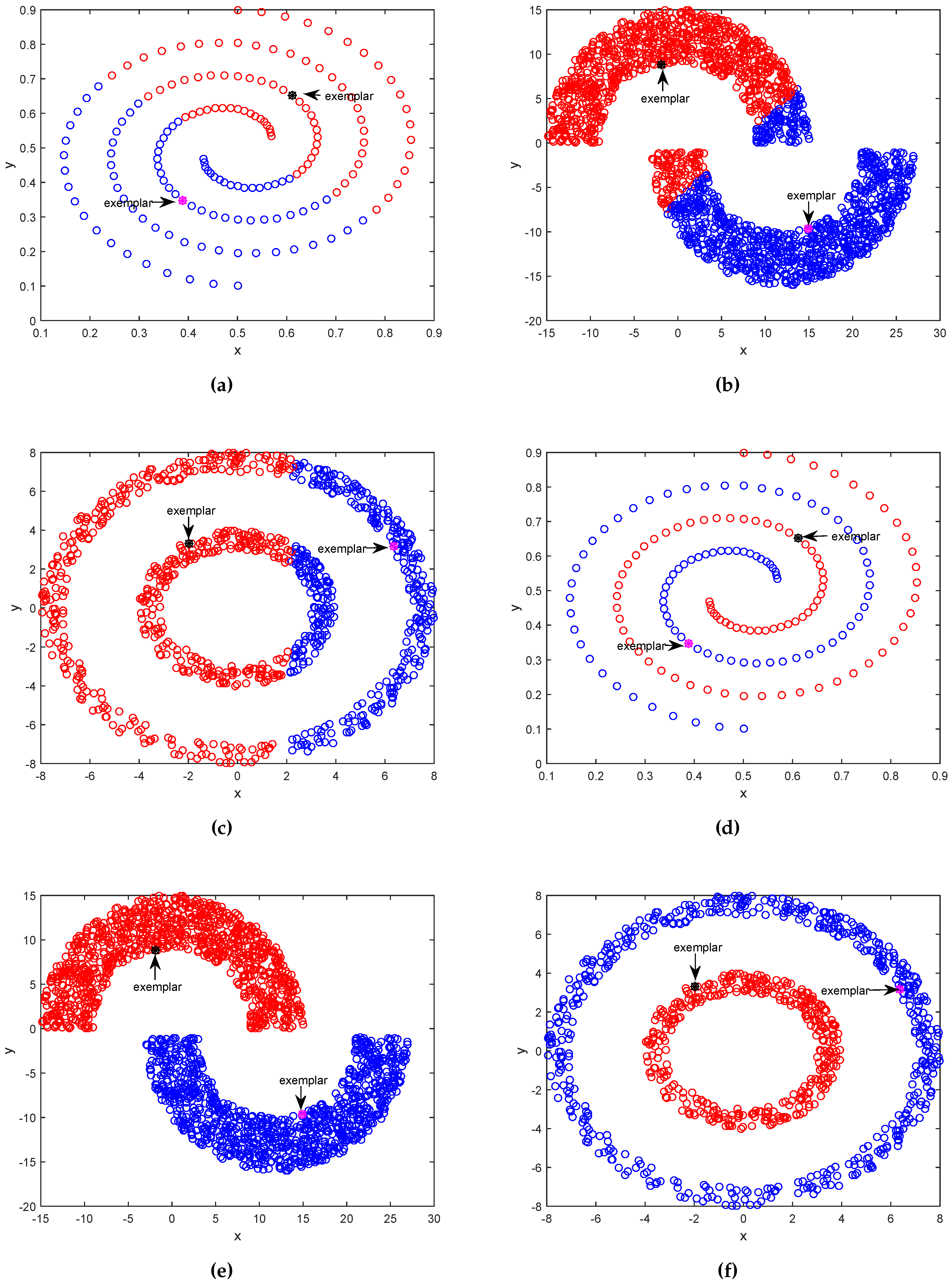
In this section, to comparatively and visually study the difference between APC and APC-PS, we generate three representative synthetic datasets, whose samples are distributed with different complex structures. The first dataset has two spirals, the second includes two half-moons, and the third has two circles with different radiuses.
In Figure 2a, we can see APC equally cuts two spirals and does not identify the cluster structure of samples. In Figure 2b, APC correctly groups most samples, but it still wrongly assigns some samples. In Figure 2c, APC divides two circles into two semi-circles: left and right semicircles. Obviously, APC does not correctly discover the underlying cluster structure of samples. The reason is that after finding out center samples (or exemplars), APC employs negative Euclidean distance between non-center samples and center samples, and assigns non-center samples to their closest center samples. The Euclidean distance and assignment rule ignore the underlying structure of samples, especially for samples distributed with complex structures. On the contrary, in Figure 2d, APC-PS accurately groups samples into two interwound spirals. In Figure 2e, APC-PS precisely assigns samples into two different half-moons. In Figure 2f, APC-PS also perfectly divide samples into two circles without any mistake. Different from APC, APC-PS correctly reveals the underlying cluster structure of these three datasets.
From these comparisons, we can conclude that APC-PS can more correctly identify the underlying cluster structure of samples than APC. This occurs principally because path-based similarity not only takes into account Euclidean distance between samples, but also the longest segment along the path between samples, to explore the structure of samples. For example, although Figure 2a,d have the same exemplars, the results of APC and APC-PS are quite different. APC assigns no-exemplar samples based on their Euclidean distance from exemplars. Samples are assigned to the cluster whose exemplar is closest to them, irrespective of how these samples distributed. In contrast, APC-PS assigns non-exemplar samples to a cluster based on path-based similarity between the cluster exemplar and these samples. As Figure 2d shows, the path-based similarity between blue samples and purple exemplar is larger than the path-based similarity between blue samples and black exemplar. Therefore, blue samples is assigned to the cluster, whose center sample is the purple exemplar, and APC-PS can get more accurate results than APC.
The path-based similarity in APC-PS is quite different from the well known Floyd Warshall algorithm [27], which finds shortest paths for any pairwise nodes in a not fully connected graph with positive (or negative) edge weights. On the contrary, our proposed path-based similarity mainly focuses on path-based similarity between exemplars and other samples, and assumes there are direct edges between all samples. In addition, it first finds out all the longest segments of all paths connecting an exemplar and another sample, and then chooses the shortest segment from these found longest segments as the path-based similarity between them. If we adopt the Floyd’s shortest path to cluster samples in Figure 2a–c, the shortest path between an exemplar and a non-exemplar is the direct edge connecting them, instead of the summed edge weight of a path, which connects them via other intermediate samples. Therefore, Floyd’s shortest path produces similar clustering results as APC based on negative Euclidean distance. Furthermore, APC-PS only computes the path-based similarity between center samples and non-center samples, its time complexity is , k is the number of exemplars. However, the time complexity of original Floyd Warshall algorithm is and that for pAPC is also . Therefore, the path-based similarity adopted by APC-PS takes much less time than Floyd Warshall algorithm and pAPC.
3.2. Results on UCI Datasets
In this section, we conduct two kinds of experiments on UCI datasets [25]. In Section 3.2.1, we compare APC-PS with original APC [8], pAPC [21], APCGD [22], k-means [28], expectation maximization (EM) [29,30] and subspace sparse clustering (SSC) [31] to study the effectiveness of APC-PS. In the following experiments, λ for APC, APC-PS, pAPC and APCGD is set as 0.9, k for APC, APC-PS, pAP, APCGD, SSC, k-means and EM is fixed as the number of ground truth labels. For APCGD, the number of nearest neighbors and ε is predefined based on the scale of dataset. The number of nearest neighbors is 10 for Balance, Glass, Synthetic, and 20 for Mushroom. ε for APCGD is set as 5 on Balance, Glass, Synthetic, and is 10 on Mushrooms. We investigate the influence of different input values of p for APC-PS and APC in Section 3.2.2. These experiments are involved with four UCI datasets, Balance scale, Glass identification, Synthetic control chart time series and Mushrooms datasets. Detail information of these four datasets is listed in Table 1.
Two evaluation metrics are adopted to evaluate the quality of clusterings, F-measure [32,33] and Fowlkes-Mallows Index (FMI) [34]. F-measure is the harmonic average of precision (Prec) and recall (Rec). Suppose n samples are categorized by l classes and grouped into k clusters by a clustering algorithm. and represents the set of samples in the -th (). The precision for -th class () and is , and recall is . is the number of samples in cluster , is the number of samples labeled with and is the number of samples whose label is and assigned to cluster . The FMeasure between class and cluster is:
The overall F-measure of is:
FMI is another commonly-used metric for clustering [34] and defined as:
where a is the number of samples of the same label and grouped into the same cluster, b is the number of samples of the same label but grouped into different clusters, and c is the number of samples of different labels but grouped in the same cluster.
3.2.1. Clustering results on UCI datasets
In this section, we take APC, k-means [28], EM [29,30] , SSC [31], pAPC [21] and APCGD [22] as the comparing methods and comparatively study the performance of APC-PS on four UCI datasets. To avoid random effect, we repeat the experiments 20 times for each comparing method on each dataset, and report the average results and standard deviations in Table 2 and Table 3. Since pAPC can not finish on Mushroom in 12 days, its results on Mushroom are not reported in these two tables. In these table, the numbers in boldface denote the statistical significant best (or comparable best) results at 95% confident level.
From Table 2 and Table 3, we have clear observation that none of these comparing algorithms are always performing better than others. This is because different algorithms have different bias and these adopted four datasets are also distributed with different structures.
EM is outperformed by k-means, APC and APC-PS in majority cases. The reason is that EM assumes samples are normally distributed. But samples in these four datasets are not subject to normal distribution. k-means outperforms SSC on Synthetic control and Glass identification, but it loses to SSC on other two datasets. The reason is that k-means can work well on spherical datasets, but it does not perform well on other datasets, whose samples are distributed with complex structures. Although SSC assumes the sparsity of features and mixture of subspace clusters, it is still often loses to APC and always loses to APC-PS. The possible cause is that the assumption used by SSC does not hold for these four datasets.
APC-PS significantly performs better than APC in most cases under different evaluation metrics and it often performs as well as the best of the other five methods in terms of F-measure and FMI. APC only utilizes Euclidean distance between samples to explore the underlying structures between samples. In contrast, APC-PS not only exploits the Euclidean distance, but also a path-based similarity to explore the underlying structures of samples and to assign samples to their respective clusters via this similarity. Therefore, APC-PS produces better results than APC. From these results, we can draw a conclusion that the path-based similarity can faithfully explore underlying structures of samples and thus to boost the accuracy of APC.
APCGD and pAPC adopts different techniques to measure the similarity between samples, instead of the original negative Euclidean distance. They are still outperformed by APC-PS in most cases. APC-PS and pAPC employ similar path-based similarity to assign a non-exemplar sample to the cluster, whose exemplar has largest similarity with the sample. APC-PS achieves better results than pAPC. This occurs principally because APC-PS and pAPC take different samples as exemplars. In practice, pAPC computes the path-based similarity between any pairwise samples at first. Then, it performs APC based on this similarity. In contrast, APC-PS firstly finds out the exemplar for each cluster using the negative Euclidean distance between samples. Next, it calculates the path-based similarity between the found exemplars and other samples. This observation suggests APC-PS can more correctly find out exemplars than pAPC. APCGD defines a neighborhood graph at first, and then it takes the shortest path between two samples in the graph as the geodesic distance between them. Next, APCGD takes the negative geodesic distance as the similarity between them and performs APC based on this similarity. Obviously, if two samples are directly connected in the graph, the shortest path between two samples is the direct edge. However, it is rather difficult to construct a suitable neighborhood graph for APCGD, and an inappropriate neighborhood graph can bring direct connection between two samples, which belong to two different clusters. Given that, the performance of APCGD often loses to APC-PS.
3.2.2. Sensitivity of p on APC and APC-PS
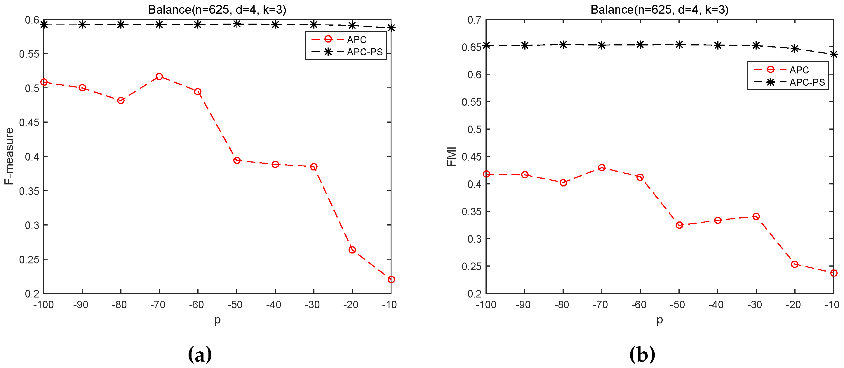
In this section, we investigate the sensitivity of APC and APC-PS on the input values of p. For this purpose, we vary p from −100 to −10 on Balance and vary p from −200 to −110, since the number of exemplars is equal (or close) to k in the chosen range.
From Figure 3, we can easy see APC-PS is always significantly better than APC on the Balance scale dataset across the specified range of p, irrespective of F-measure or FMI. In practice, both APC and APC-PS initially identify the same exemplars, but their results are quite different. The cause is that APC-PS uses the path-based similarity to assign a non-exemplar sample to a cluster, whose exemplar is most similar to the non-exemplar sample. In contrast, APC takes the negative Euclidean distance between two samples as the similarity between them and it assigns a non-exemplar sample to its most similar exemplar based on this similarity. This observation justifies our motivation to incorporate the path-based similarity to improve the performance of APC. In addition, we can find the performance of APC-PS in Figure 3 keeps relatively stable, whereas the performance of APC fluctuates sharply. This fact further demonstrates the path-based similarity not only helps exploring the underlying structure between samples, but also helps achieving stable results.
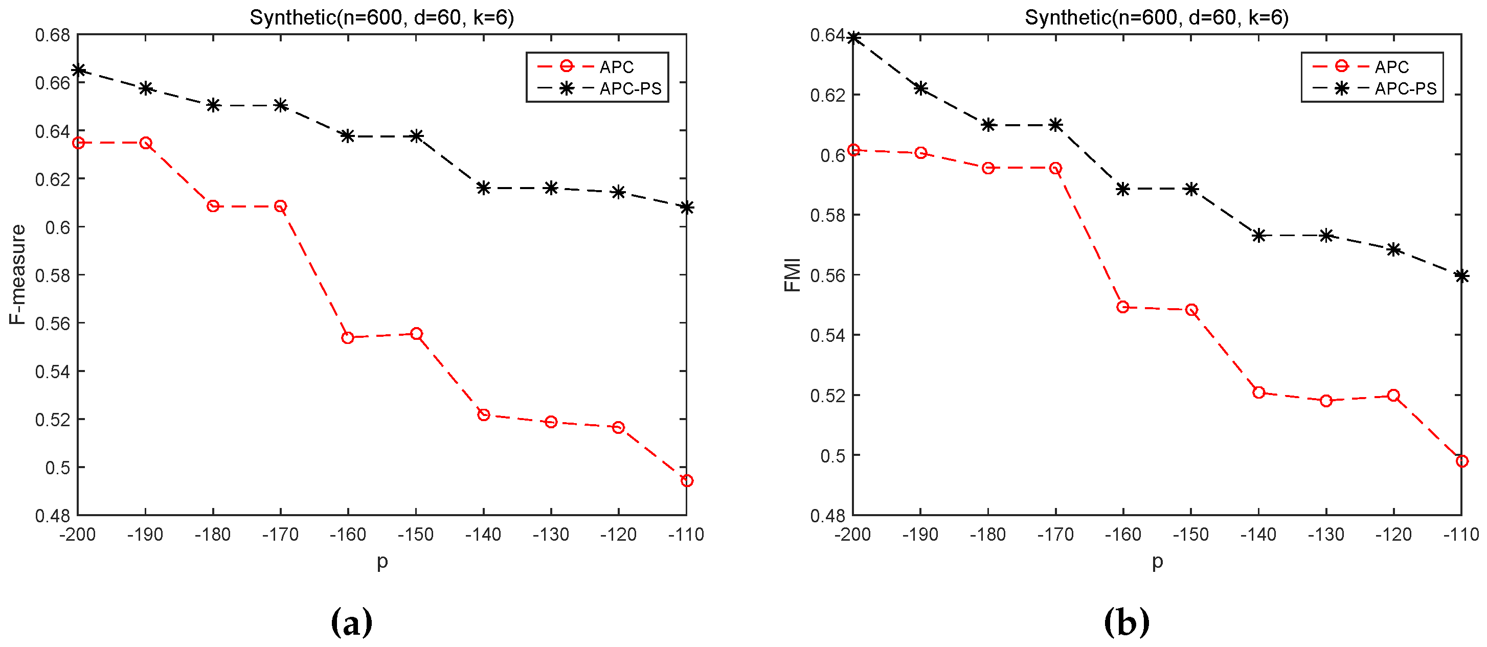
As to Figure 4, APC-PS also always produce higher results than APC on Synthetic control chart time series dataset. In fact, both APC and APC-PS are also based on the same exemplars. The performance difference between APC-PS and APC indicates the samples in Balance scale dataset and Synthetic control chart time series dataset are distributed with complex structures. These results again suggest that solely utilizing negative Euclidean distance based similarity between samples to assign non-center samples to a cluster is not so reasonable, and this similarity can assign a sample, far away from its cluster center but close to other samples in the cluster, to another cluster, whose exemplar has large similarity with the sample. On the other hand, APC-PS employs a path-based similarity. This similarity combines negative Euclidean distance based similarity and path-based similarity between exemplars and non-exemplar samples. For samples far away from a target exemplar, APC-PS considers the connection between non-exemplar samples and the exemplar. And hence, the path-based similarity can explore the structure of samples, and help APC-PS to achieve better results than APC.
Another interesting observation is that APC-PS in Figure 4 does not show as stable results as that in Figure 4. APC-PS fluctuates similarly as APC in Figure 4. One explanation is that the identified exemplars are changed as p varying. p also influences the availability matrix and response matrix . However, since APC-PS additionally employs the path-based similarity, it still correctly assigns more samples to their respective clusters, thus it gets better results than APC. In summary, we can say that APC-PS is more robust to input values of p than APC.
4. Conclusions
In this paper, to improve the performance of APC on samples distributed with complex structures, we introduce an algorithm called affinity propagation clustering based on path-based similarity (APC-PS). The experimental results on synthetic datasets and UCI datasets show APC-PS outperforms other related algorithms, and it is also robust to input values of p. Our study shows the path-based similarity can help to explore the underlying cluster of samples and thus to improve the performance of APC. In our future work, we will investigate other similarity measures to capture the local and global structure of samples, and to boost the performance of APC.
Acknowledgments
This work is supported by Natural Science Foundation of China (No. 61402378), Natural Science Foundation of CQ CSTC (cstc2014jcyjA40031 and cstc2016jcyjA0351), Fundamental Research Funds for the Central Universities of China (2362015XK07 and XDJK2016B009).
Author Contributions
Yuan Jiang and Yuliang Liao performed the experiments, Yuan Jiang drafted the manuscript; Guoxian Yu proposed the idea, conceived the whole process and revised the manuscript; All the authors read and approved the final manuscript.
Conflicts of Interest
The authors declare no conflict of interest.
References
- Napolitano, F.; Raiconi, G.; Tagliaferri, R.; Ciaramella, A.; Staiano, A.; Miele, G. Clustering and visualization approaches for human cell cycle gene expression data analysis. Int. J. Approx. Reason. 2008, 47, 70–84. [Google Scholar] [CrossRef]
- Peng, W.F.; Du, S.; Li, F.X. Unsupervised image segmentation via affinity propagation. Appl. Mech. Mater. 2014, 610, 464–470. [Google Scholar] [CrossRef]
- Kang, J.H.; Lerman, K.; Plangprasopchok, A. Analyzing microblogs with affinity propagation. In Proceedings of the First Workshop on Social Media Analytics (SOMA ‘10), Washington, DC, USA, 25 July 2010; pp. 67–70.
- Hong, L.; Cai, S.M.; Fu, Z.Q.; Zhou, P.L. Community identification of financial market based on affinity propagation. In Recent Progress in Data Engineering and Internet Technology; Springer: Berlin, Germany, 2013; pp. 121–127. [Google Scholar]
- Papalexakis, E.E.; Beutel, A.; Steenkiste, P. Network anomaly detection using co-clustering. In Encyclopedia of Social Network Analysis and Mining; Springer: New York, NY, USA, 2014; pp. 1054–1068. [Google Scholar]
- Ester, M.; Kriegel, H.P.; Sander, J.; Xu, X. A density-based algorithm for discovering clusters in large spatial databases with noise. In Proceedings of the 2nd International Conference on Knowledge Discovery and Data Mining, Portland, OR, USA, 2–4 August 1996; Volume 96, pp. 226–231.
- Rodriguez, A.; Laio, A. Clustering by fast search and find of density peaks. Science 2014, 344, 1492–1496. [Google Scholar] [CrossRef] [PubMed]
- Frey, B.J.; Dueck, D. Clustering by passing messages between data points. Science 2007, 315, 972–976. [Google Scholar] [CrossRef] [PubMed]
- Frey, B.J.; Dueck, D. Response to comment on “Clustering by passing messages between data points”. Science 2008, 319, 726. [Google Scholar] [CrossRef]
- Zhang, R. Two similarity measure methods based on human vision properties for image segmentation based on affinity propagation clustering. In Proceedings of the International Conference on Measuring Technology and Mechatronics Automation (ICMTMA), Changsha, China, 13–14 March 2010; Volume 3, pp. 1054–1058.
- Du, H.; Wang, Y.P.; Duan, L.L. A new method for grayscale image segmentation based on affinity propagation clustering algorithm. In Proceedings of the IEEE 9th International Conference on Computational Intelligence and Security, Leshan, China, 14–15 Decebmer 2013; pp. 170–173.
- Leone, M.; Sumedha; Weigt, M. Clustering by soft-constraint affinity propagation: Applications to gene-expression data. Bioinformatics 2007, 23, 2708–2015. [Google Scholar] [CrossRef] [PubMed]
- Zhao, C.W.; Peng, Q.K.; Zhao, C.W.; Sun, S.H. Chinese text automatic summarization based on affinity propagation cluster. In Proceedings of the International Conference on Fuzzy Systems and Knowledge Discovery, Tianjin, China, 14–16 August 2009; Volume 1, pp. 425–429.
- Xiao, Y.; Yu, J. Semi-supervised clustering based on affinity propagation algorithm. J. Softw. 2008, 19, 2803–2813. [Google Scholar] [CrossRef]
- Wagstaff, K.; Cardie, C.; Rogers, S.; Schrödl, S. Constrained k-means clustering with background knowledge. In Proceedings of the 18th International Conference on Machine Learning, Williamstown, MA, USA, 28 June–1 July 2001; pp. 577–584.
- Wang, K.J.; Zhang, J.Y.; Li, D.; Zhang, X.N.; Guo, T. Adaptive affinity propagation clustering. Acta Autom. Sin. 2007, 33, 1242–1246. [Google Scholar]
- Xia, D.Y.; Fei, W.U.; Zhang, X.Q.; Zhuang, Y.T. Local and global approaches of affinity propagation clustering for large scale data. J. Zhejiang Univ. Sci. A 2008, 9, 1373–1381. [Google Scholar] [CrossRef]
- Serdah, A.M.; Ashour, W.M. Clustering large-scale data based on modified affinity propagation algorithm. J. Artif. Intell. Soft Comput. Res. 2016, 6, 23–33. [Google Scholar] [CrossRef]
- Zhang, X.L.; Wang, W.; Norvag, K.; Sebag, M. K-AP: Generating specified K clusters by efficient affinity propagation. In Proceedings of the IEEE Tenth International Conference on Data Mining (ICDM), Sydney, Australia, 13–17 December 2010; pp. 1187–1192.
- Barbakh, W.; Fyfe, C. Inverse weighted clustering algorithm. Comput. Inf. Syst. 2007, 11, 10–18. [Google Scholar]
- Walter, S.F. Clustering by Affinity Propagation. Ph.D. Thesis, ETH Zurich, Zürich, Switzerland, 2007. [Google Scholar]
- Zhang, L.; Du, Z. Affinity propagation clustering with geodesic distances. J. Computat. Inf. Syst. 2010, 6, 47–53. [Google Scholar]
- Guo, K.; Guo, W.; Chen, Y.; Qiu, Q.; Zhang, Q. Community discovery by propagating local and global information based on the MapReduce model. Inf. Sci. 2015, 323, 73–93. [Google Scholar] [CrossRef]
- Meo, P.D.; Ferrara, E.; Fiumara, G.; Ricciardello, A. A novel measure of edge centrality in social networks. Knowl.-Based Syst. 2012, 30, 136–150. [Google Scholar] [CrossRef]
- Lichman, M. UCI Machine Learning Repository. 2013. Available online: http://www.ics.uci.edu/ml (accessed on 21 July 2016).
- Jain, A.K. Data clustering: 50 years beyond k-means. Pattern Recognit. Lett. 2010, 31, 651–666. [Google Scholar] [CrossRef]
- Floyd, R.W. Algorithm 97: Shortest path. Commun. ACM 1962, 5, 345. [Google Scholar] [CrossRef]
- MacQueen, J. Some methods for classification and analysis of multivariate observations. In Proceedings of the 5th Berkeley Symposium on Mathematical Statistics and Probability, Oakland, CA, USA, 21 June–18 July 1965 and 27 December 1965–7 January 1966; Volume 1, pp. 281–297.
- Dempster, A.P.; Laird, N.M.; Rubin, D.B. Maximum likelihood from incomplete data via the EM algorithm. J. R. Stat.Soc. Ser. B (Methodol.) 1977, 39, 1–38. [Google Scholar]
- Bradley, P.S.; Fayyad, U.; Reina, C. Scaling EM (eXpectation-Maximization) Clustering to Large Databases; Technical Report, MSR-TR-98-35; Microsoft Research Redmond: Redmond, WA, USA, 1998. [Google Scholar]
- Elhamifar, E.; Vidal, R. Sparse subspace clustering: algorithm, theory, and applications. IEEE Trans. Pattern Anal. Mach. Intell. 2013, 35, 2765–2781. [Google Scholar] [CrossRef] [PubMed]
- Larsen, B.; Aone, C. Fast and effective text mining using linear-time document clustering. In Proceedings of the 5th ACM SIGKDD International Conference on Knowledge Discovery and Data Mining, San Diego, CA, USA, 15–18 August 1999; pp. 16–22.
- Dalli, A. Adaptation of the F-measure to cluster based lexicon quality evaluation. In Proceedings of the EACL 2003 Workshop on Evaluation Initiatives in Natural Language Processing. Association for Computational Linguistics, Budapest, Hungary, 13 April 2003; pp. 51–56.
- Halkidi, M.; Batistakis, Y.; Vazirgiannis, M. On clustering validation techniques. J. Intell. Inf. Syst. 2001, 17, 107–145. [Google Scholar] [CrossRef]
Figure 1.
A toy example: 202 samples distributed in two curves. “e1” and “e2” are the exemplars of the lower cluster and upper cluster, respectively.
Figure 1.
A toy example: 202 samples distributed in two curves. “e1” and “e2” are the exemplars of the lower cluster and upper cluster, respectively.
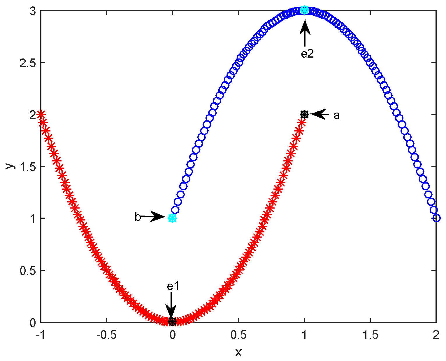
Figure 2.
Discovered clusters of affinity propagation clustering (APC) and affinity propagation clustering based on path-based similarity (APC-PS) on three artificial datasets. Upper figures (a–c) show the results of APC, and lower figures (d–f) show the results of APC-PS.
Figure 2.
Discovered clusters of affinity propagation clustering (APC) and affinity propagation clustering based on path-based similarity (APC-PS) on three artificial datasets. Upper figures (a–c) show the results of APC, and lower figures (d–f) show the results of APC-PS.

Figure 3.
APC and APC-PS on Balance scale dataset under different values of p. (a) F-measure; (b) FMI.
Figure 3.
APC and APC-PS on Balance scale dataset under different values of p. (a) F-measure; (b) FMI.

Figure 4.
APC and APC-PS on Synthetic control chart dataset under different values of p. (a) F-measure; (b) FMI.
Figure 4.
APC and APC-PS on Synthetic control chart dataset under different values of p. (a) F-measure; (b) FMI.


| Dataset | n | d | k |
|---|---|---|---|
| Balance | 625 | 4 | 3 |
| Glass | 214 | 9 | 6 |
| Synthetic | 600 | 60 | 6 |
| Mushrooms | 8124 | 112 | 2 |
Table 2.
Experimental results (average ± standard deviation) on UCI datasets under evaluation metric Fmeasure. The numbers in boldface denote the best performance.
| Method | Balance Scale | Synthetic Control | Glass Identification | Mushrooms |
|---|---|---|---|---|
| EM | 0.5718 ± 0.0020 | 0.5950 ± 0.0531 | 0.5096 ± 0.0291 | 0.6798 ± 0.1030 |
| k-means | 0.5652 ± 0.0328 | 0.6662 ± 0.0240 | 0.5364 ± 0.0234 | 0.7740 ± 0.1368 |
| SSC | 0.5728 ± 0.0000 | 0.5926 ± 0.0000 | 0.4840 ± 0.0012 | 0.7934 ± 0.0000 |
| pAPC | 0.5638 ± 0.0987 | 0.6477 ± 0.0000 | 0.4971 ± 0.0000 | —————— |
| APCGD | 0.5829 ± 0.1021 | 0.4192 ± 0.0000 | 0.4248 ± 0.0297 | 0.5781 ± 0.0000 |
| APC | 0.5518 ± 0.0563 | 0.6350 ± 0.0000 | 0.5598 ± 0.0000 | 0.7616 ± 0.0000 |
| APC-PS | 0.5925 ± 0.0018 | 0.6650 ± 0.0000 | 0.5620 ± 0.0000 | 0.7634 ± 0.0000 |
Table 3.
Experimental results (average ± standard deviation) on four datasets under evaluation metric Fowlkes-Mallows Index (FMI). The numbers in boldface denote the best performance.
| Method | Balance Scale | Synthetic Control | Glass Identification | Mushrooms |
|---|---|---|---|---|
| EM | 0.4708 ± 0.0130 | 0.5581 ± 0.0545 | 0.4516 ± 0.0397 | 0.6086 ± 0.0828 |
| k-means | 0.4567 ± 0.0241 | 0.6277 ± 0.0251 | 0.4775 ± 0.0464 | 0.7232 ± 0.1106 |
| SSC | 0.4675 ± 0.0000 | 0.5664 ± 0.0000 | 0.3778 ± 0.0005 | 0.6732 ± 0.0000 |
| pAPC | 0.5076 ± 0.1039 | 0.5664 ± 0.0000 | 0.3895 ± 0.0000 | —————— |
| APCGD | 0.5173 ± 0.0872 | 0.4750 ± 0.0000 | 0.4912 ± 0.0239 | 0.5198 ± 0.0000 |
| APC | 0.4294 ± 0.0449 | 0.6015 ± 0.0000 | 0.5606 ± 0.0000 | 0.7105 ± 0.0000 |
| APC-PS | 0.6539 ± 0.0046 | 0.6390 ± 0.0000 | 0.5477 ± 0.0000 | 0.7277 ± 0.0000 |
© 2016 by the authors; licensee MDPI, Basel, Switzerland. This article is an open access article distributed under the terms and conditions of the Creative Commons Attribution (CC-BY) license (http://creativecommons.org/licenses/by/4.0/).
Share and Cite
MDPI and ACS Style
Jiang, Y.; Liao, Y.; Yu, G. Affinity Propagation Clustering Using Path Based Similarity. Algorithms 2016, 9, 46. https://doi.org/10.3390/a9030046
AMA Style
Jiang Y, Liao Y, Yu G. Affinity Propagation Clustering Using Path Based Similarity. Algorithms. 2016; 9(3):46. https://doi.org/10.3390/a9030046
Chicago/Turabian StyleJiang, Yuan, Yuliang Liao, and Guoxian Yu. 2016. "Affinity Propagation Clustering Using Path Based Similarity" Algorithms 9, no. 3: 46. https://doi.org/10.3390/a9030046
Note that from the first issue of 2016, this journal uses article numbers instead of page numbers. See further details here.