
Designing a Framework to Improve Time Series Data of Construction Projects: Application of a Simulation Model and Singular Spectrum Analysis

Abstract
:1. Introduction
2. Literature Review
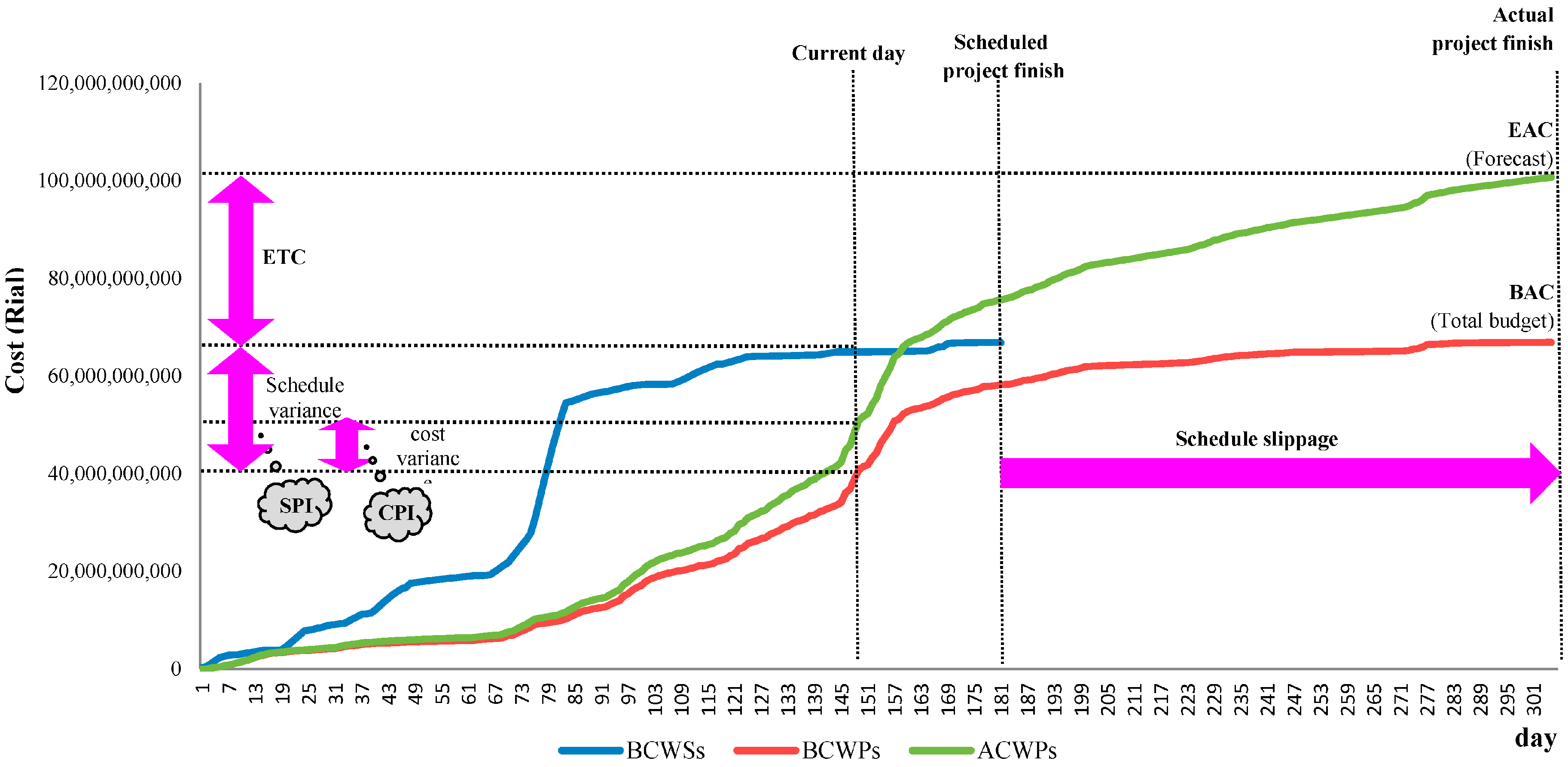
2.1. EVM
- ■
- Budgeted Cost of Work scheduled ()
- ■
- Actual Costs Work Performed (ACWP)
- ■
- Budgeted Cost of Work Performed ()
- ■
- Earned schedule (ES)
- ■
- Schedule Variance (SV = )
- ■
- Schedule Performance Index (SPI = )
- ■
- Cost Variance (CV = )
- ■
- Cost Performance Index (CPI = )
- ■
- EDAC = PD/SPI
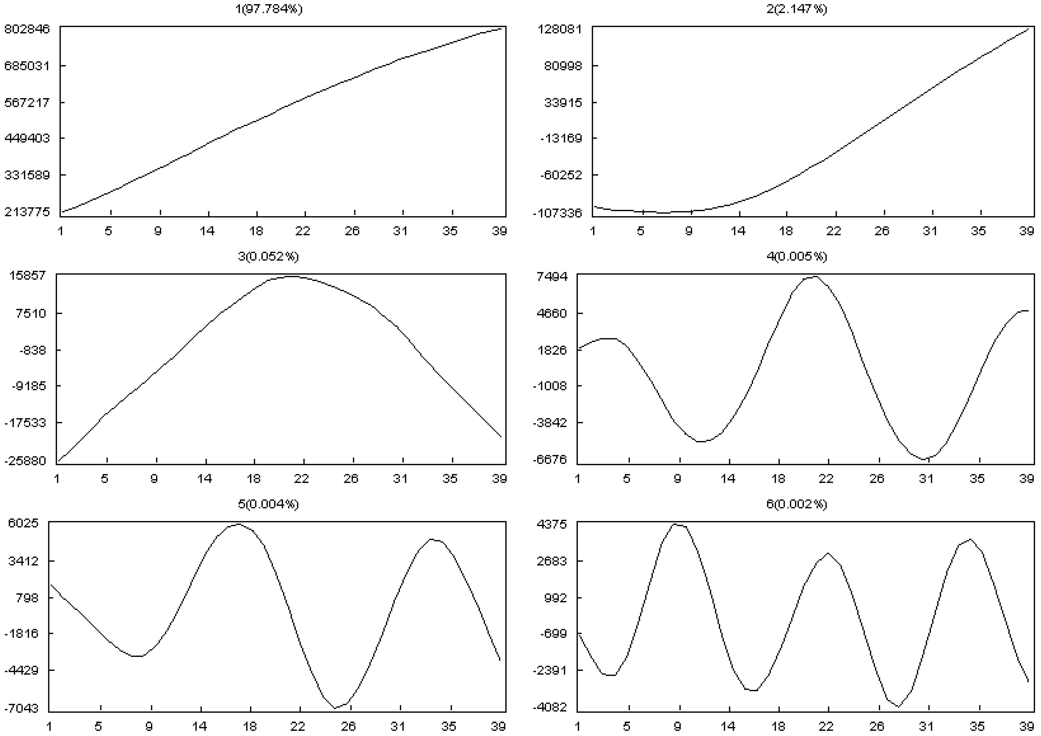
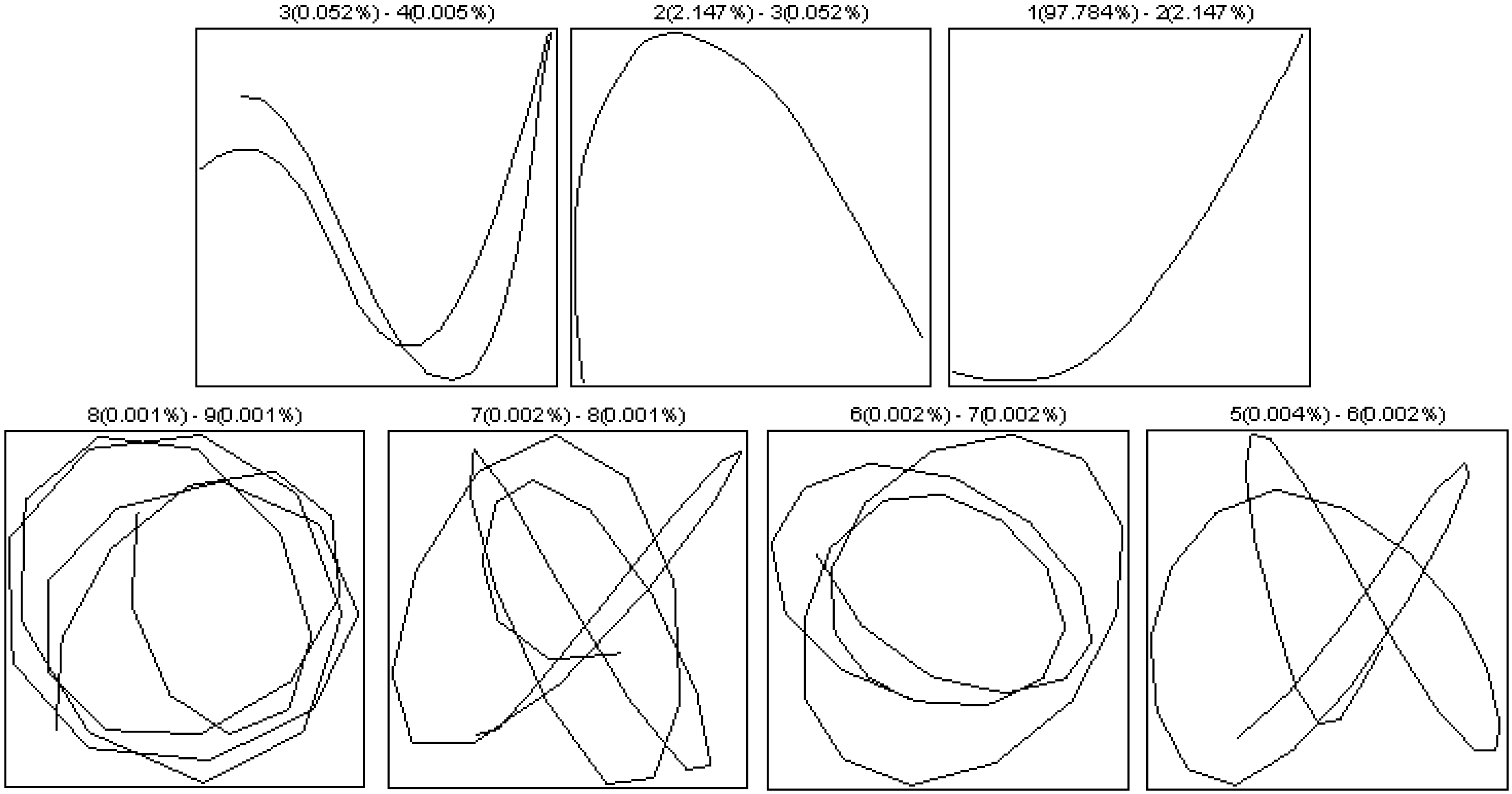
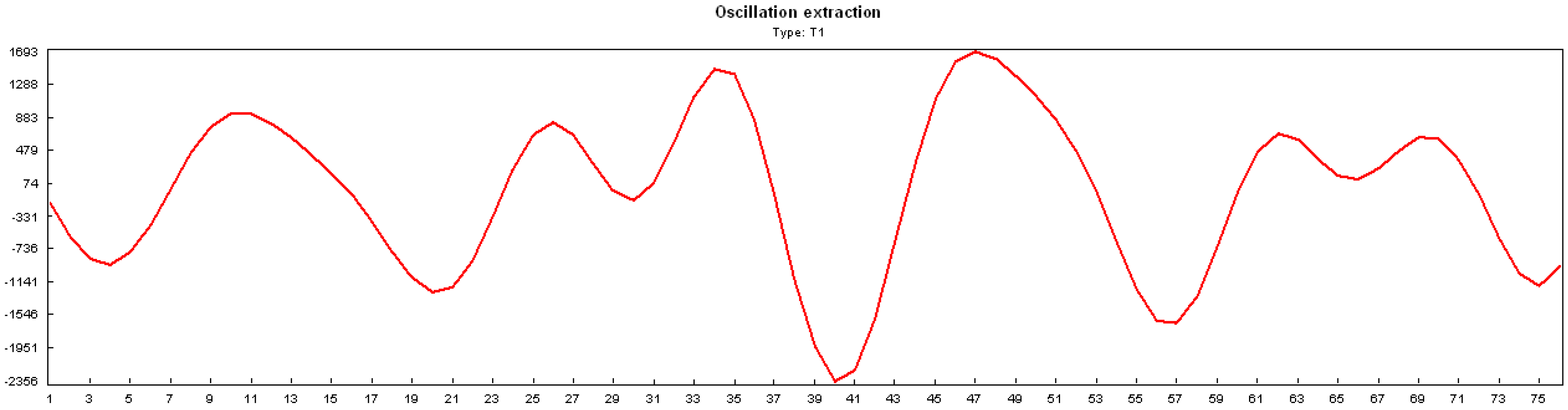
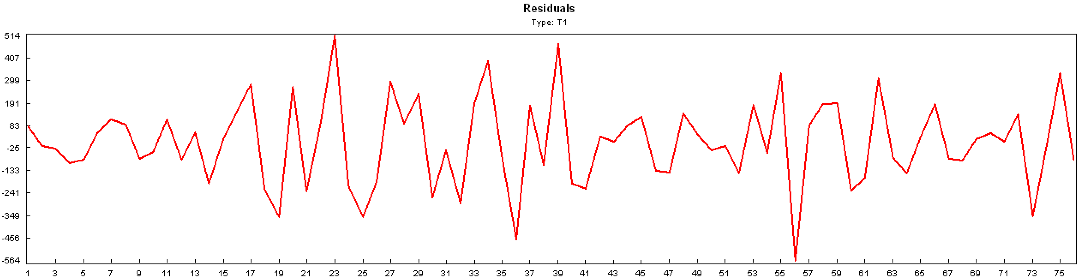
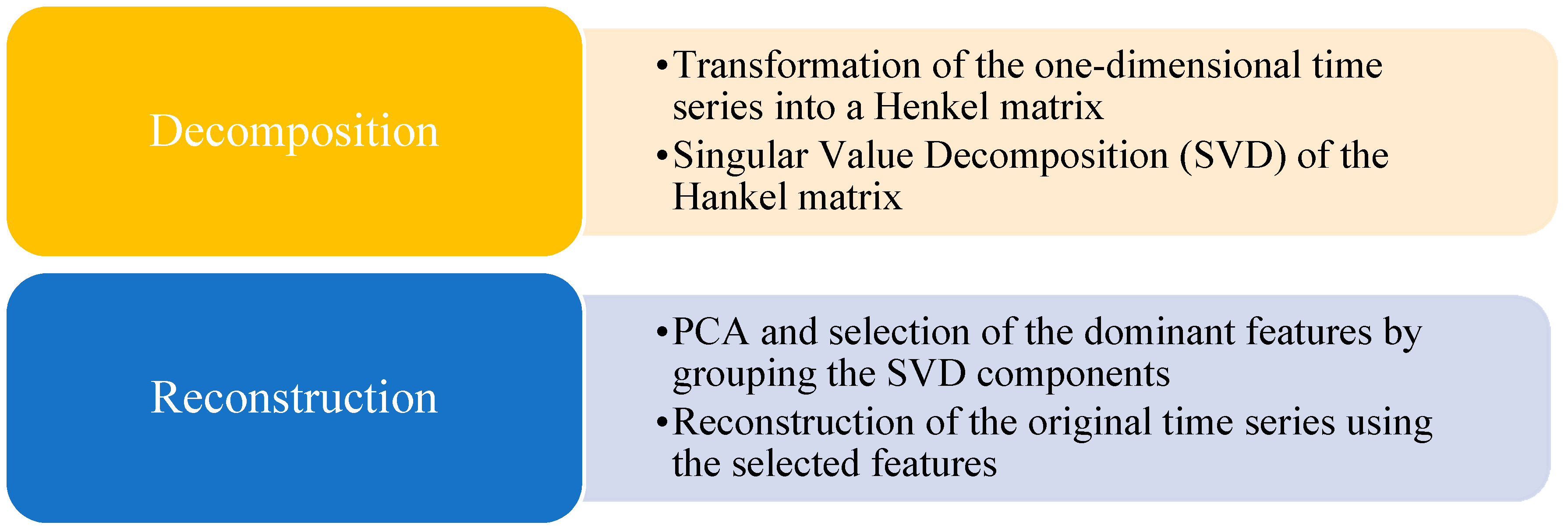
2.2. SSA
2.3. Simulation Project Techniques
3. Methodology
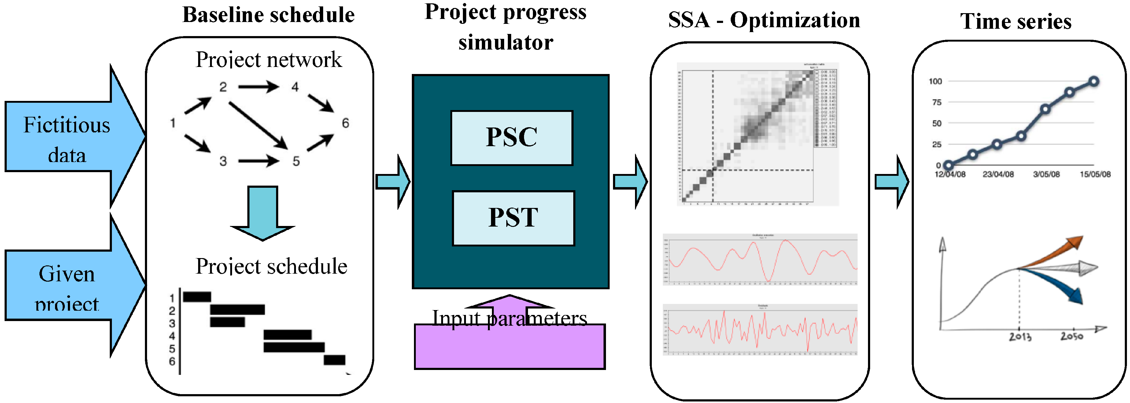
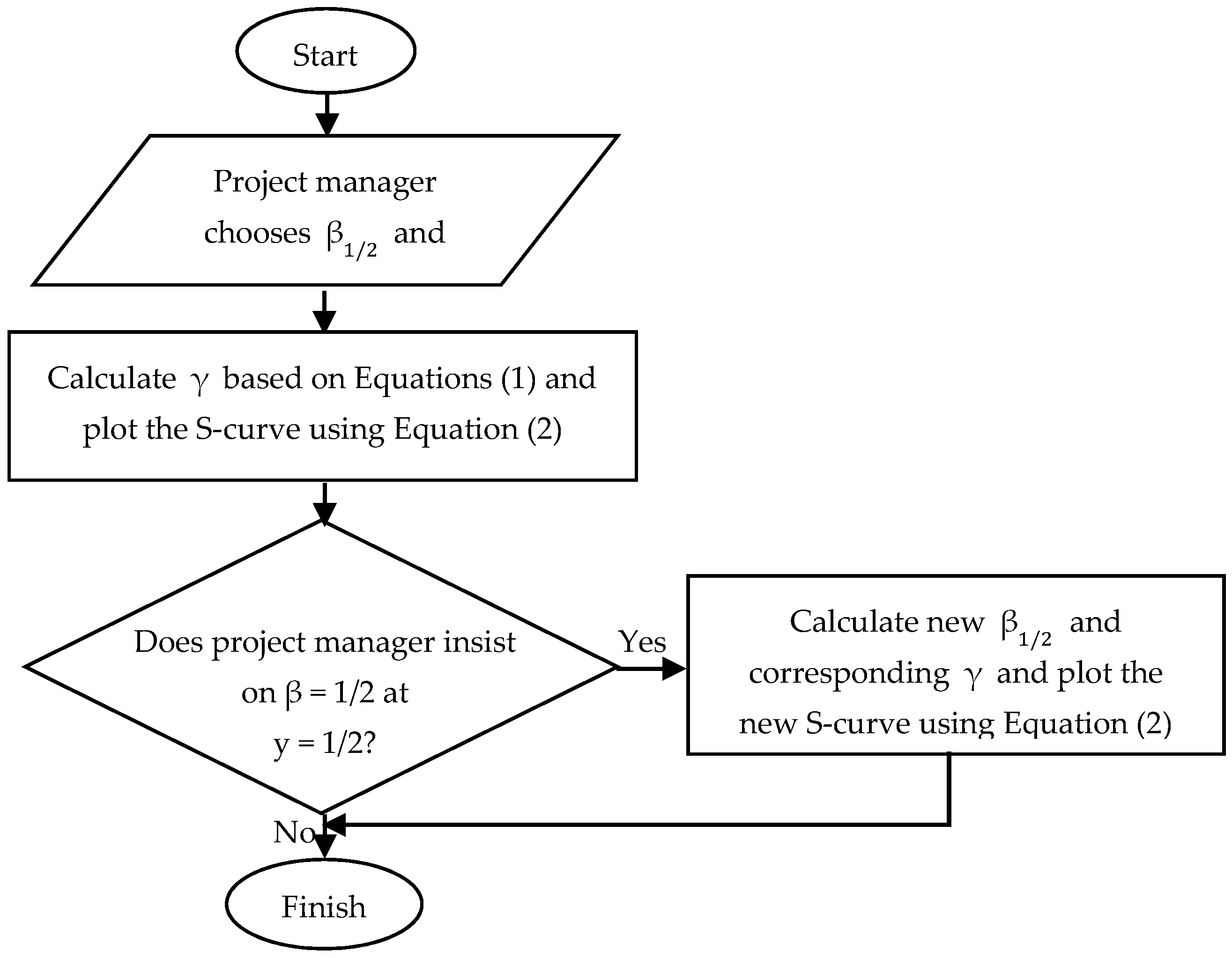
3.1. Project Progress Generator Framework
- Progress Simulation for Time (PST): PST calculates different indices in various time sections and focuses on time parameters to simulate the progress of projects.PST consists of the following steps:
- a.
- Determining the input project and parameters;
- b.
- Constructing project scheduling;
- c.
- Updating the project’s progress daily;
- d.
- Computing the project’s actual progress daily, based on the set inputs. Suppose represents the random impact of risk overall, then The impact of risk events, , integrated with the above task progress is shown as follows:where i and j represent the number of tasks and days, respectively. The random overall impact, , shows the risk of each task in each day from its start to finish. Furthermore, are daily scheduled progress in a planned day, s, and experts’ proposed status for the task, i.
- e.
- Calculating different measurement indices (i.e., EVM measurements);
- f.
- Continuing until the project is entirely completed.
- Progress Simulation for Cost (PSC): PSC simulates the progress of projects via cost progress during project execution, calculates different indices in different time sections and focuses on cost parameters. PSC is developed mainly based on the PST structure and focuses on the cost parameters. The following is a list of other principles of PSC.
- Determining the input costing parameters;
- Calculating planned cost progress based on a general specification (i.e., inflation rate) and each task’s specifications (i.e., costs of resources);
- The daily cost of each task is calculated based on resource consumption of the task on that day and other costing parameters;
- The daily project cost is calculated until the project is finished.
3.2. Input Parameters
3.3. Output Validation
- The total cost of the project (Y1);
- The total life time of the project (t1);
- The point of time when the project has spent half of its total funds (t1/2).
4. Data Description
4.1. Fictitious Project Data
4.2. Empirical Project Data
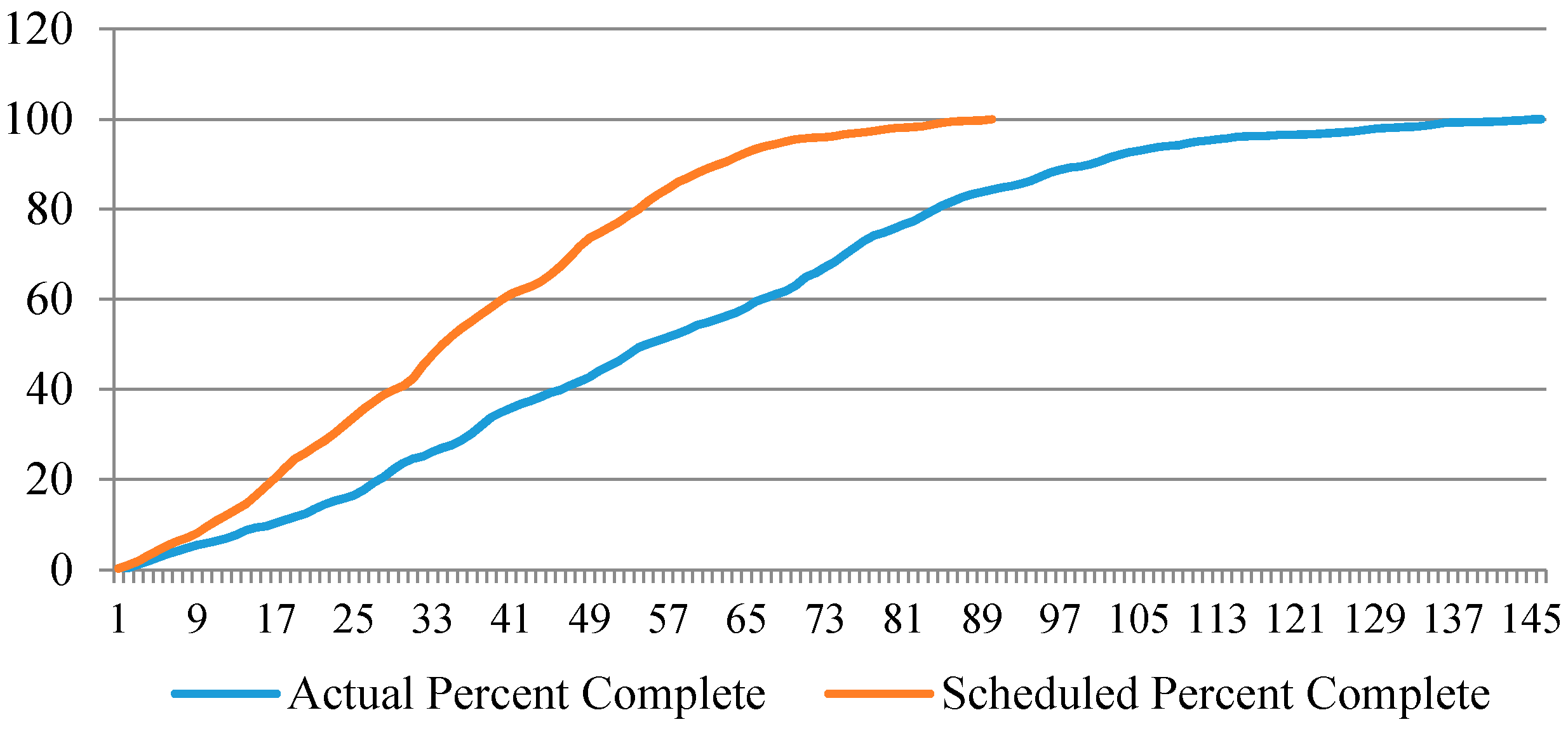
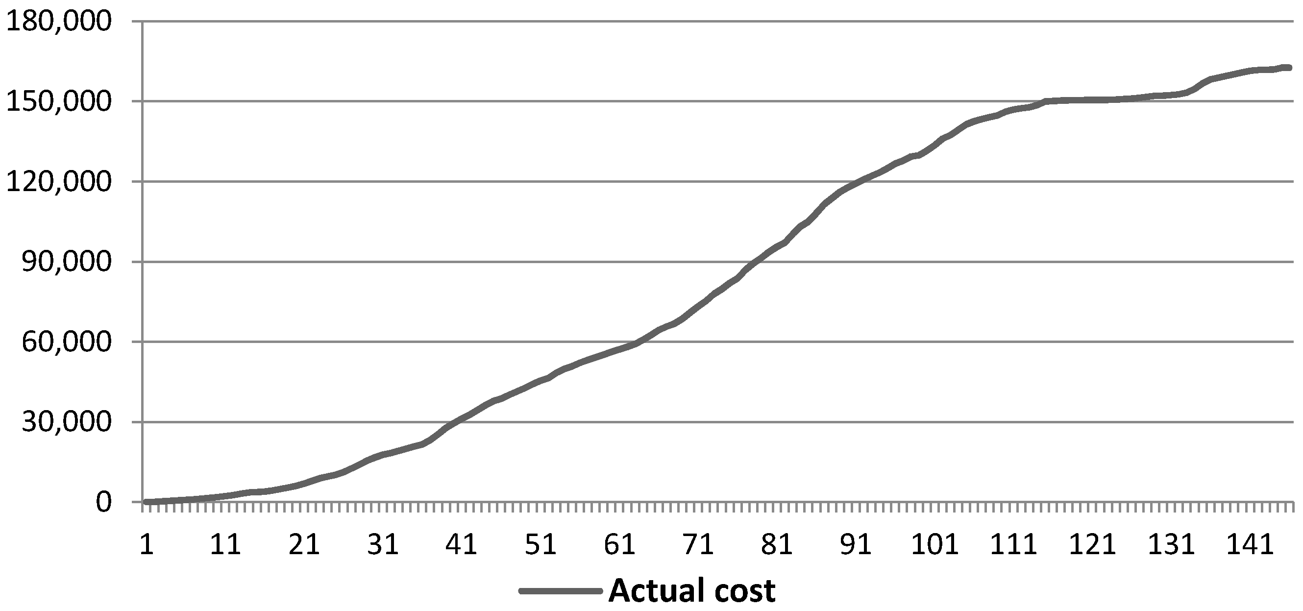
5. Simulation Result
5.1. Fictitious Project Results
- -
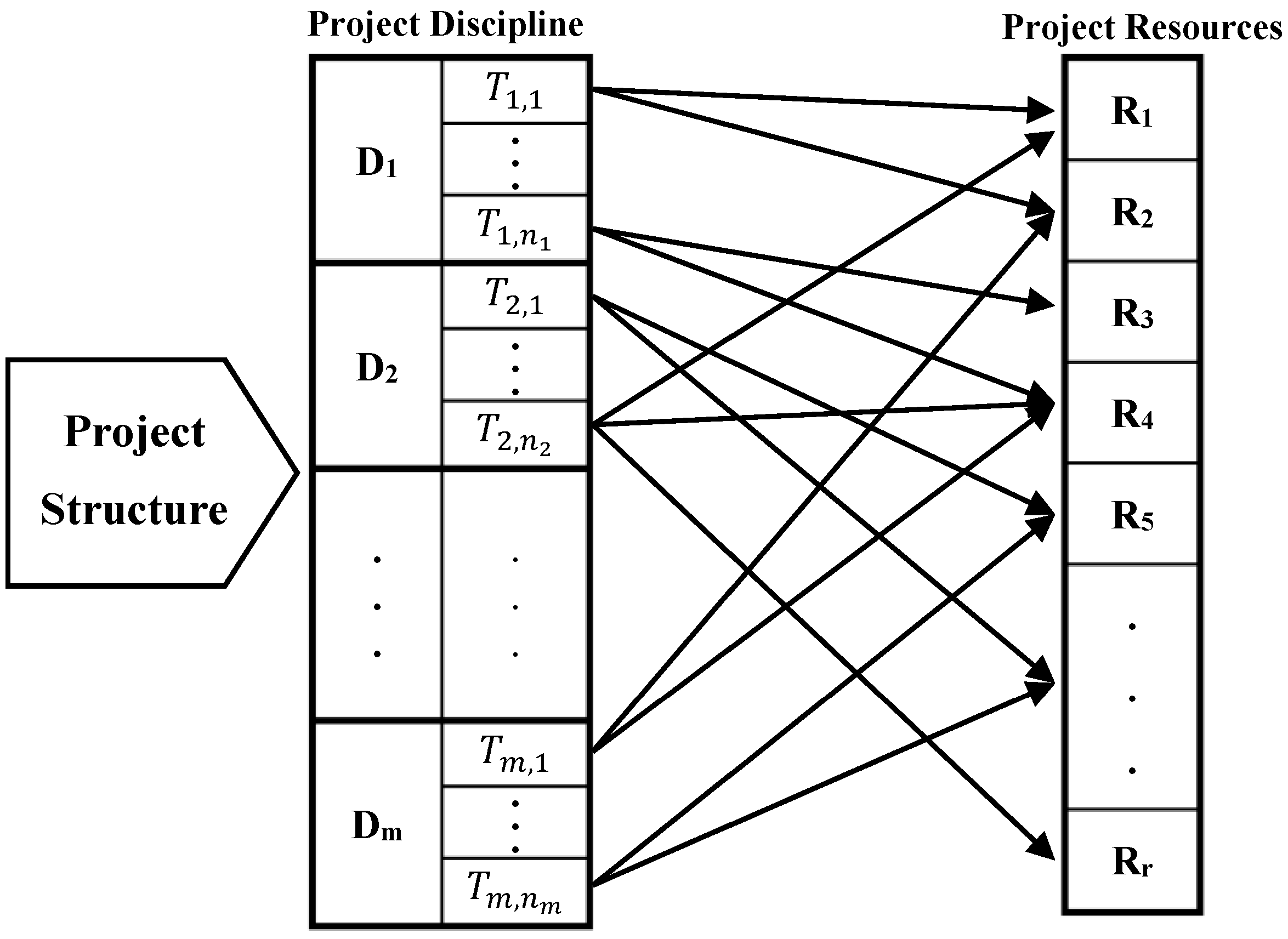
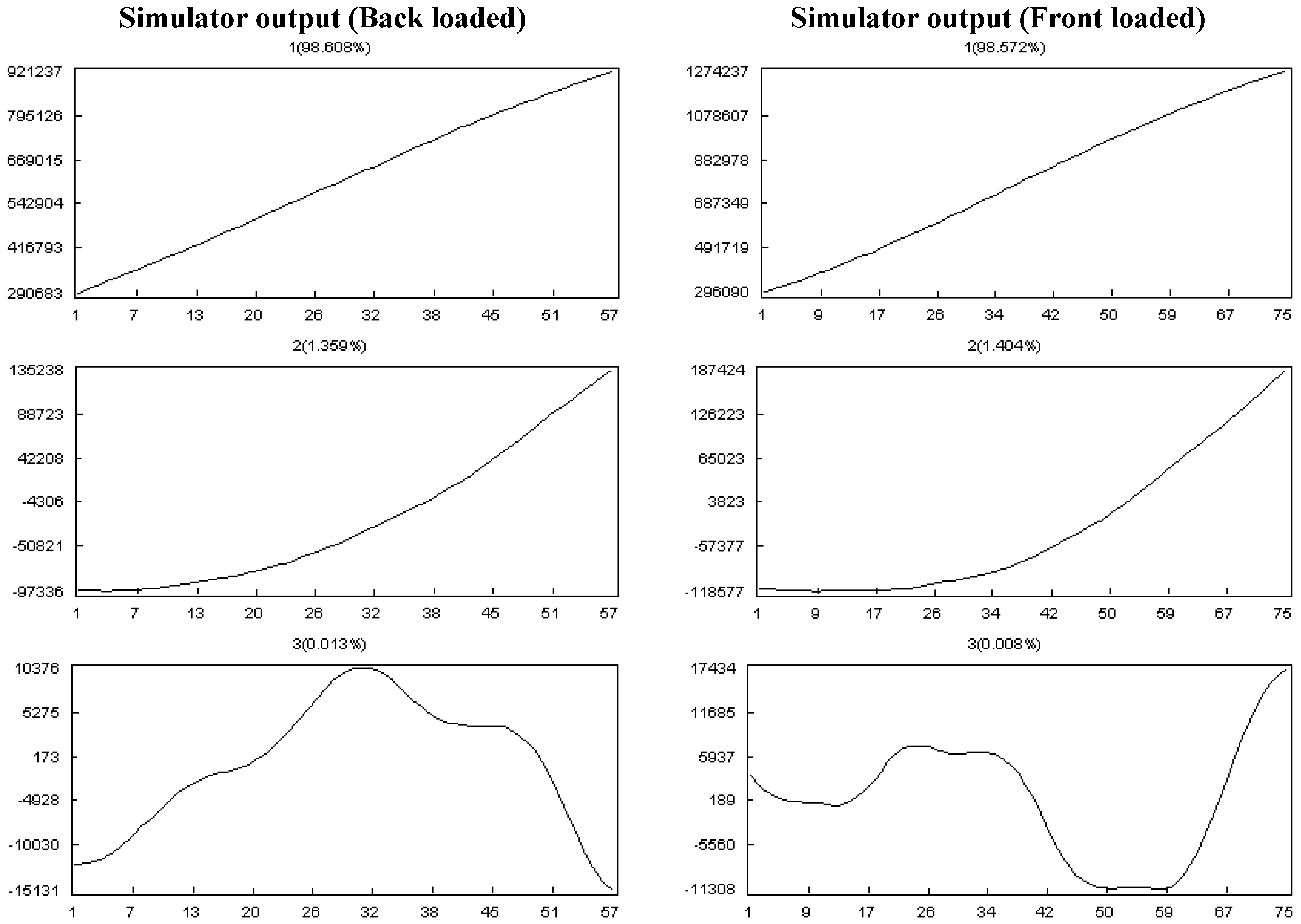
- The project has four disciplines comprising 20%, 10%, 40% and 30% of all of the tasks, and back-loaded, flat, front-loaded and bell are their work contours, respectively.
- -
- Eighty percent of task delays are in the range of 10% of scheduled progress.
- -
- The project was simulated with a 20% inflation rate for the last six months.
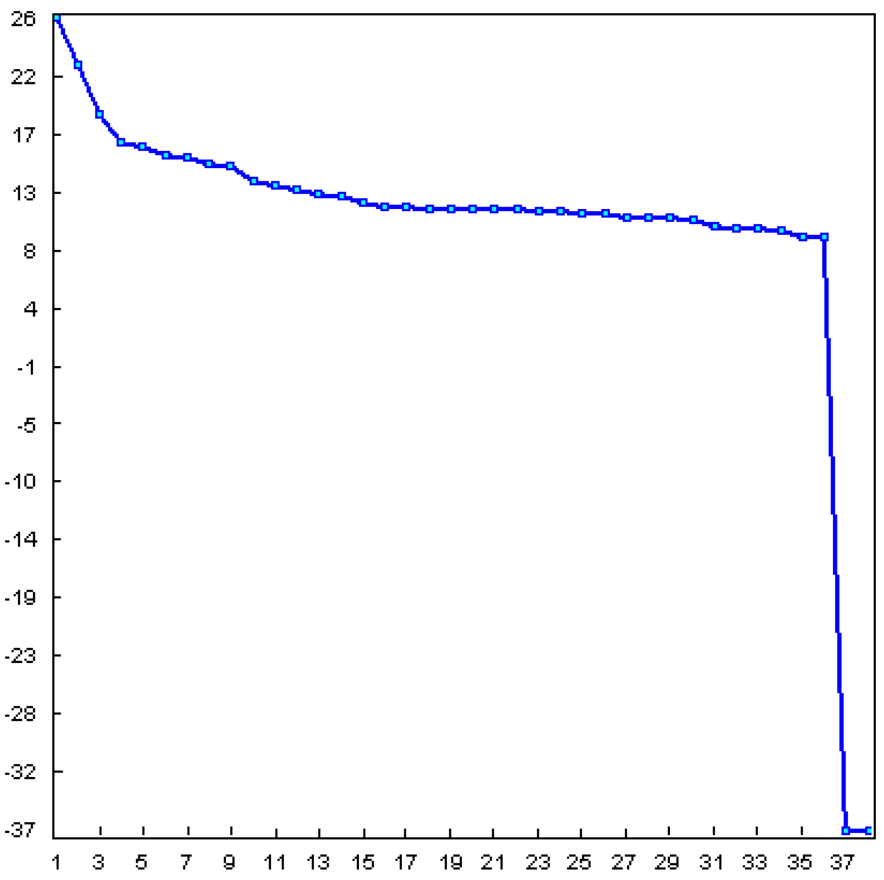
- Selection of the window length L:
- Selection of r:
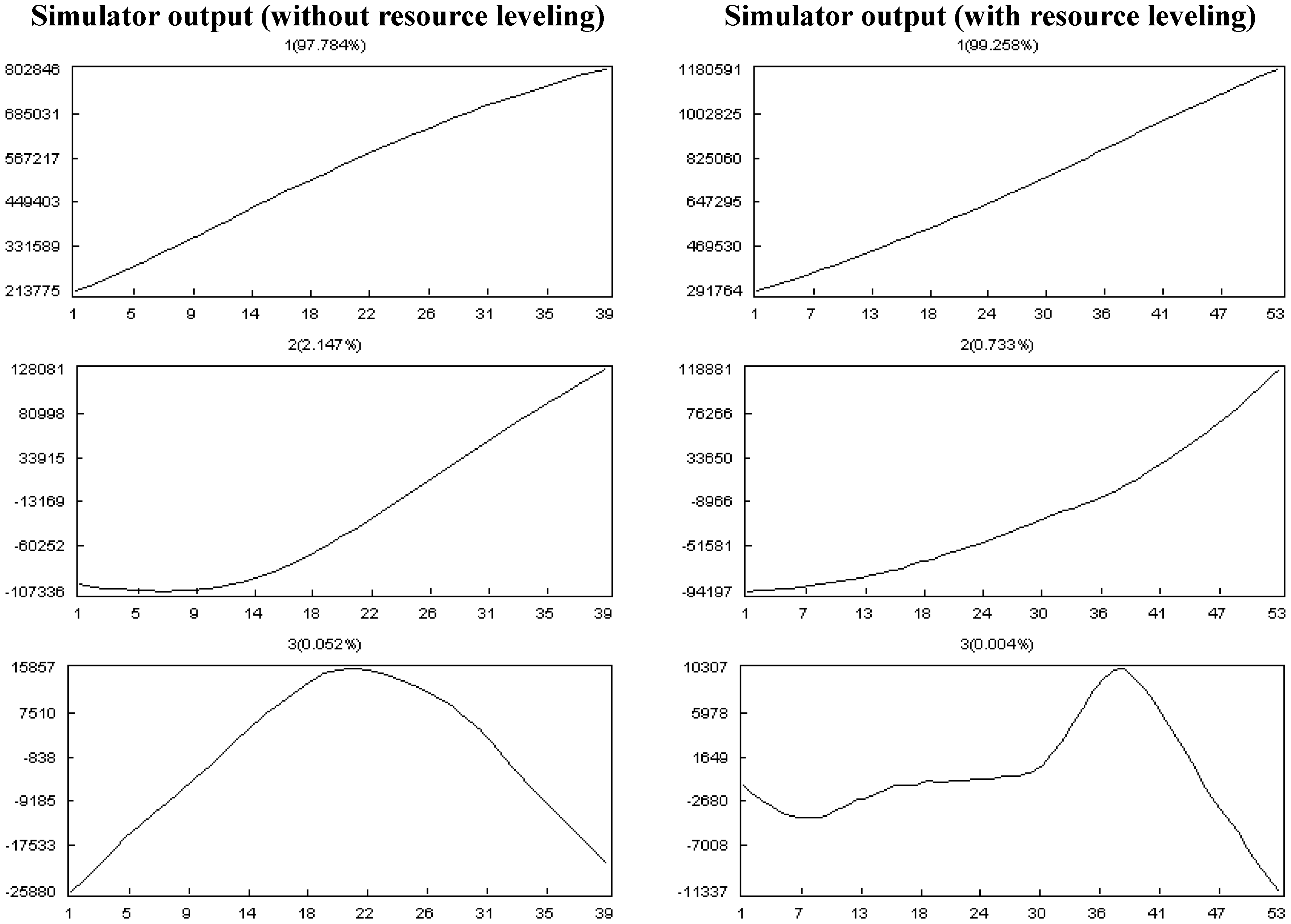
5.1.1. Effect of Input Parameters on the Simulator Results
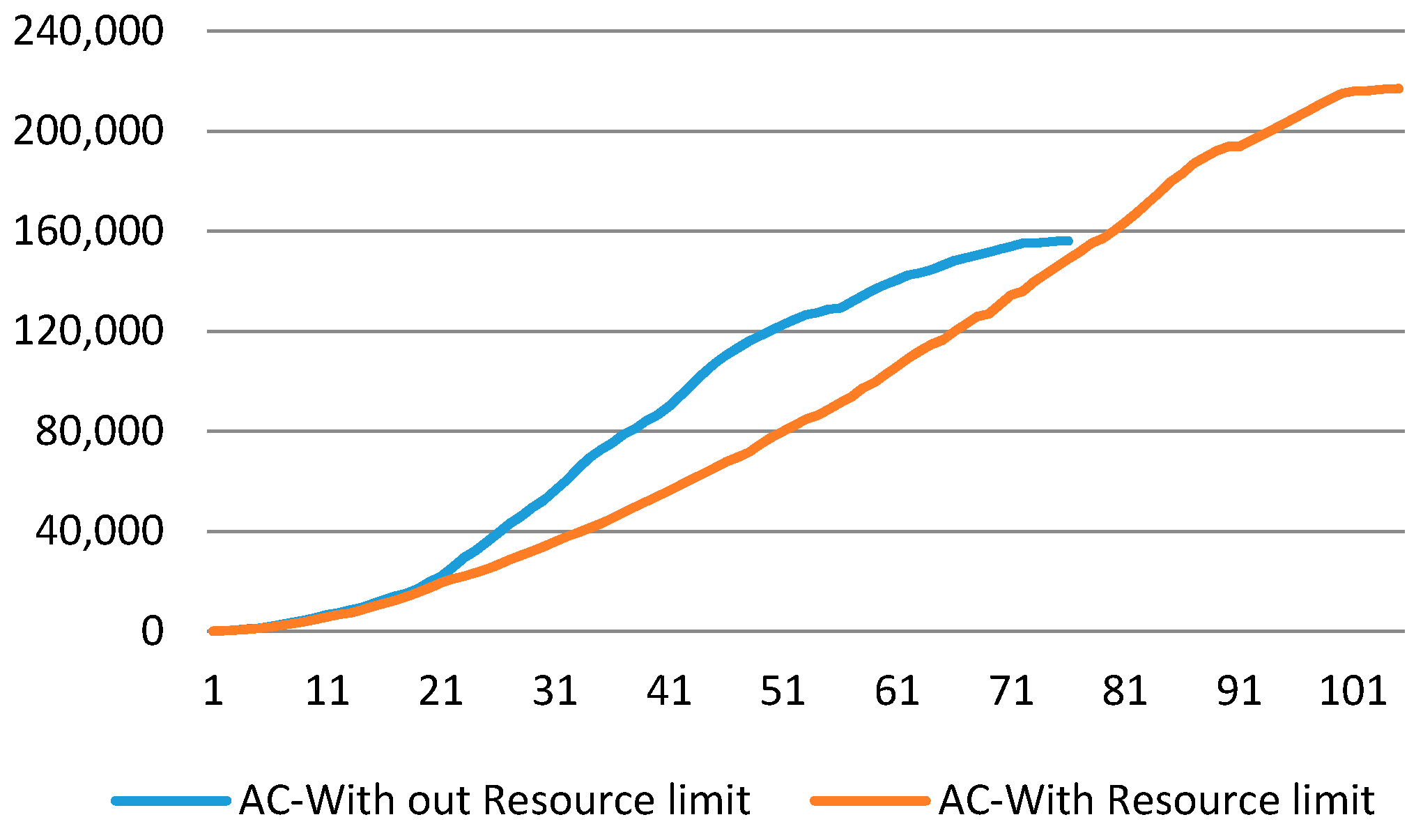
- Effect of Resource Constrains:
- Effect of discipline and work contour:
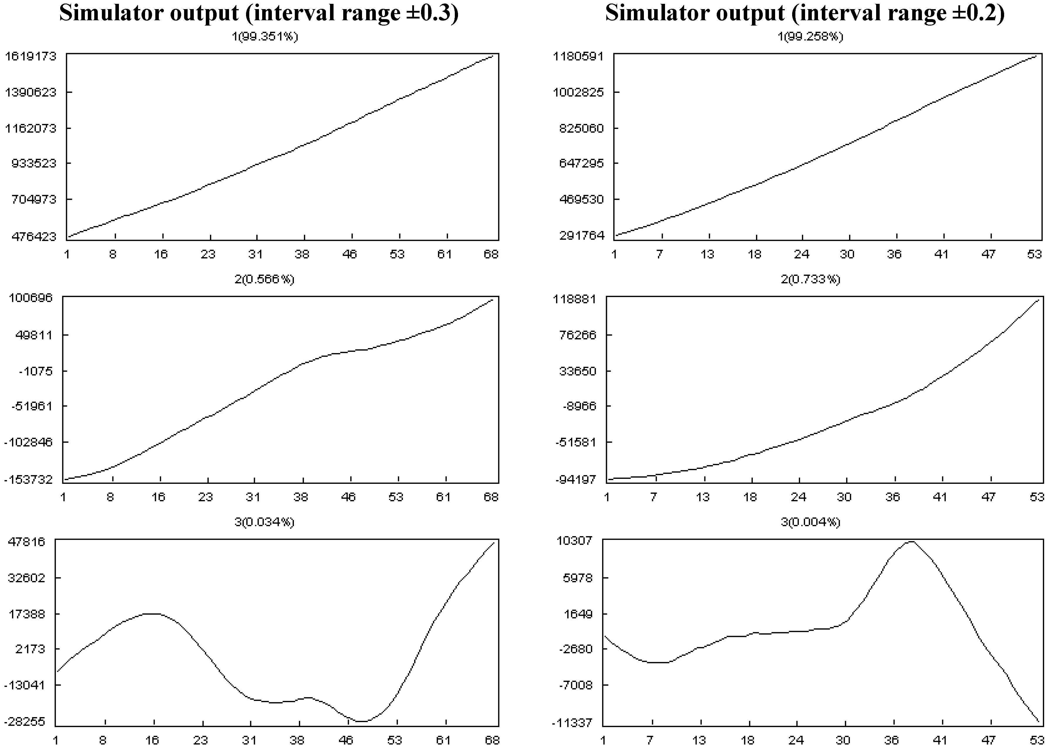
- Effect of the changes in the progress status:
- ■
- The actual progress of tasks fluctuates ±0.2 of their plan progress.
- ■
- The actual progress of tasks fluctuates ±0.3 of their plan progress.
5.2. Case Study Results
6. Conclusions
Acknowledgments
Author Contributions
Conflicts of Interest
References
- Kolisch, R.; Sprecher, A. PSPLIB—A project scheduling problem library. Eur. J. Oper. Res. 1996, 96, 205–216. [Google Scholar] [CrossRef]
- Kolisch, R.; Padman, R. An Integrated Survey of Project Management Scheduling; Technical Report; Heinz School of Public Policy and Management, Carnegie Mellon University: Pittsburgh, PA, USA, 1997. [Google Scholar]
- Hartmann, S.; Briskorn, D. A survey of variants and extensions of the resource-constrained project scheduling problem. Eur. J. Oper. Res. 2010, 207, 1–15. [Google Scholar] [CrossRef]
- Kolisch, R.; Hartmann, S. Experimental investigation of heuristics for resource-constrained project scheduling: An update. Eur. J. Oper. Res. 2006, 174, 23–37. [Google Scholar] [CrossRef]
- Vanhoucke, M. Measuring the efficiency of project control using fictitious and empirical project data. Int. J. Proj. Manag. 2012, 30, 252–263. [Google Scholar] [CrossRef]
- Cioffi, D. Designing project management: A scientific notation and an improved formalism for earned value calculations. Int. J. Proj. Manag. 2006, 24, 136–144. [Google Scholar] [CrossRef]
- Iranmanesh, S.H.; Kimiagari, S.; Mojir, N. A new formula to estimate at completion of a project’s time to improve earned value management system. In Proceedings of the IEEE International Conference on Industrial Engineering and Engineering Management (IEEM), Singapore, 2–4 December 2007; pp. 1014–1020.
- Madadi, M.; Iranmanesh, H. A management-oriented approach to reduce project duration and its risk (variability). Eur. J. Oper. Res. 2012, 215, 751–761. [Google Scholar] [CrossRef]
- Fleming, Q.W.; Koppleman, J.M. Earned Value Project Management; Project Management Institute: Newtown Square, PA, USA, 1996. [Google Scholar]
- Lipke, W.; Zwikael, O.; Henderson, K.; Anbari, F. Prediction of project outcome: the application of statistical methods to earned value management and earned schedule performance indexes. Int. J. Proj. Manag. 2009, 27, 400–407. [Google Scholar] [CrossRef]
- Fleming, Q.; Koppelman, J. What’s your project’s real price tag? Harv. Bus. Rev. 2003, 81, 20–21. [Google Scholar]
- Jacob, D.S.; Kane, M. Forecasting schedule completion using earned value metrics. Meas. News 2004, 3, 11–17. [Google Scholar]
- Vandevoorde, S.; Vanhoucke, M. A comparison of different project duration forecasting methods using earned value metrics. Int. J. Proj. Manag. 2006, 24, 289–302. [Google Scholar] [CrossRef]
- Vanhoucke, M.; Vandevoorde, S. A simulation and evaluation of earned value metrics to forecast the project duration. J. Oper. Res. Soc. 2007, 58, 1361–1374. [Google Scholar] [CrossRef]
- Iranmanesh, S.H.; Tavassoli, H.Z. Intelligent systems in project performance measurement and evaluation. In Engineering Management, intelligent systems references library 87; Springer International Publishing: Basel, Switzerland, 2015. [Google Scholar] [CrossRef]
- Elshaer, R. Impact of sensitivity information on the prediction of project’s duration using earned schedule method. Int. J. Proj. Manag. 2013, 31, 579–588. [Google Scholar] [CrossRef]
- Hassani, H.; Ghodsi, Z.; Silva, E.S.; Heravi, S. From nature to maths: Improving forecasting performance in subspace-based methods using genetics Colonial Theory. Dig. Signal Process. 2016, 51, 101–109. [Google Scholar] [CrossRef]
- Golyandina, N.; Nekrutkin, V.; Zhigljavsky, A. Analysis of Time Series Structure: SSA and Related Techniques; Chapman & Hall/CRC: Boca Raton, FL, USA, 2001. [Google Scholar]
- Hassani, H. Singular Spectrum Analysis: Methodology and comparison. J. Data Sci. 2007, 5, 239–257. [Google Scholar]
- Hassani, H.; Zokaei, M.; von Rosen, D.; Amiri, S.; Ghodsi, M. Does noise reduction matter for curve fitting in growth curve models? Comput. Methods Progr. Biomed. 2009, 96, 173–181. [Google Scholar] [CrossRef] [PubMed]
- Viljoen, H.; Nel, D.G. Common singular spectrum analysis of several time series. J. Stat. Plan. Inference 2010, 140, 260–267. [Google Scholar] [CrossRef]
- Hassani, H.; Heravi, S.; Zhigljavsky, A. Forecasting European industrial production with singular spectrum analysis. Int. J. Forecast. 2009, 25, 103–118. [Google Scholar] [CrossRef]
- Afshar, K.; Bigdeli, N. Data analysis and short-term load forecasting in Iran’s electricity market using singular spectral analysis (SSA). Energy 2011, 36, 2620–2627. [Google Scholar] [CrossRef]
- Silva, E.S. A combination forecast for energy-related CO2 emissions in the United States. Int. J. Energy Stat. 2013, 1, 269–279. [Google Scholar] [CrossRef]
- Ghodsi, Z.; Silva, E.S.; Hassani, H. Bicoid signal extraction with a selection of parametric and nonparametric signal processing techniques. Genom. Proteom. Bioinform. 2015, 13, 183–191. [Google Scholar] [CrossRef] [PubMed] [Green Version]
- Wu, C.L.; Chau, K.W. Rainfall-Runoff Modeling Using Artificial Neural Network Coupled with Singular Spectrum Analysis. J. Hydrol. 2001, 399, 394–409. [Google Scholar] [CrossRef]
- Chau, K.W.; Wu, C.L. A Hybrid Model Coupled with Singular Spectrum Analysis for Daily Rainfall Prediction. J. Hydroinform. 2010, 12, 458–473. [Google Scholar] [CrossRef]
- Hassani, H.; Mahmoudvand, R.; Zokaei, M. Separability and window length in singular spectrum analysis. C. R. Acad. Sci. Paris Ser. I. 2011, 349, 987–990. [Google Scholar] [CrossRef]
- Hanna, M.; Ruwanpura, J.Y. Simulation tool for manpower forecast loading and resource leveling. In Proceedings of the 2007 Winter Simulation Conference, Washington, DC, USA, 9–12 December 2007; pp. 2099–2103.
- Al-Jibouri, S.H. Monitoring systems and their effectiveness for project cost control in construction. Int. J. Proj. Manag. 2003, 21, 145–154. [Google Scholar] [CrossRef]
- Huang, E.; Chen, S.J. Estimation of project completion time and factors analysis for concurrent engineering project management: A simulation approach. Concurr. Eng. Res. Appl. 2006, 14, 329–341. [Google Scholar] [CrossRef]
- Akintoye, A. Analysis of factors influencing project cost estimating practice. Constr. Manag. Econ. 2000, 18, 77–89. [Google Scholar] [CrossRef]
- Bashir, H.A.; Thomson, V. Project estimation from feasibility study until completion: A quantitative methodology. Concurr. Eng. Res. Appl. 2001, 9, 257–269. [Google Scholar] [CrossRef]
- Kuhl, M.; Radhames, A.; Pena, T. A dynamic crashing method for project management using simulation-based optimization. In Proceedings of the 40th Conference on Winter Simulation, Austin, TX, USA, 7–10 December 2008; pp. 2370–2376.
- Cioffi, D.F. A tool for managing projects: An analytic parameterization of the S-Curve. Int. J. Proj. Manag. 2005, 23, 215–222. [Google Scholar] [CrossRef]
- The ProGen standard dataset. Available online: http://129.187.106.231/psplib/main.html (accessed on 13 July 2016).
- Caterpillar-SSA Software. Available online: http://www.gistatgroup.com/cat/index.html (accessed on 13 July 2016).
- Hassani, H.; Webster, A.; Silva, E.S.; Heravi, S. Forecasting U.S. tourist arrivals using optimal Singular Spectrum Analysis. Tour. Manag. 2015, 46, 322–335. [Google Scholar] [CrossRef]


| MAX | RMSE | R | |
|---|---|---|---|
| ACWP | 156,015.81 | ||
| SSA | 158,153.98 | 1050.64 | 0.92 |
| S-Curve | 155,155.24 | 2166.50 | 0.93 |
| Time of Forecast | % Schedule Completed | % Work Completed | EDAC | ES | CV% |
|---|---|---|---|---|---|
| 1/00 | 0/32 | 0/06 | 225/90 | 0/03 | 0 |
| 32/00 | 11/36 | 17/91 | 383.08 | 0/76 | 0/34 |
| 63/00 | 35/78 | 31/84 | 584.70 | 1/88 | 0/92 |
| 94/00 | 79/50 | 45/16 | 762.57 | 0/45 | 3/17 |
| 125/00 | 92/93 | 53/02 | 448.16 | 0/53 | 8/04 |
| 156/00 | 95/39 | 62/80 | 241.40 | 0/70 | 18/94 |
| 187/00 | 100/00 | 73/21 | 27/44 |
© 2016 by the authors; licensee MDPI, Basel, Switzerland. This article is an open access article distributed under the terms and conditions of the Creative Commons Attribution (CC-BY) license (http://creativecommons.org/licenses/by/4.0/).
Share and Cite
Hojjati Tavassoli, Z.; Iranmanesh, S.H.; Tavassoli Hojjati, A. Designing a Framework to Improve Time Series Data of Construction Projects: Application of a Simulation Model and Singular Spectrum Analysis. Algorithms 2016, 9, 45. https://doi.org/10.3390/a9030045
Hojjati Tavassoli Z, Iranmanesh SH, Tavassoli Hojjati A. Designing a Framework to Improve Time Series Data of Construction Projects: Application of a Simulation Model and Singular Spectrum Analysis. Algorithms. 2016; 9(3):45. https://doi.org/10.3390/a9030045
Chicago/Turabian StyleHojjati Tavassoli, Zahra, Seyed Hossein Iranmanesh, and Ahmad Tavassoli Hojjati. 2016. "Designing a Framework to Improve Time Series Data of Construction Projects: Application of a Simulation Model and Singular Spectrum Analysis" Algorithms 9, no. 3: 45. https://doi.org/10.3390/a9030045