Improved Direct Linear Transformation for Parameter Decoupling in Camera Calibration

Abstract

For camera calibration based on direct linear transformation (DLT), the camera’s intrinsic and extrinsic parameters are simultaneously calibrated, which may cause coupling errors in the parameters and affect the calibration parameter accuracy. In this paper, we propose an improved direct linear transformation (IDLT) algorithm for calibration parameter decoupling. This algorithm uses a linear relationship of calibration parameter errors and obtains calibration parameters by moving a three-dimensional template. Simulation experiments were conducted to compare the calibration accuracy of DLT and IDLT algorithms with image noise and distortion. The results show that the IDLT algorithm calibration parameters achieve higher accuracy because the algorithm removes the coupling errors.

1. Introduction

With the technological developments of digital cameras and microprocessors, computer vision has been widely applied to robot navigation, surveillance, three-dimensional (3D) reconstruction and other fields for its high speed, high accuracy and non-contact nature. To obtain improved 3D information from a two-dimensional (2D) image, it is necessary to calibrate the intrinsic parameters of the camera, such as the focal distance and optical center point, as well its extrinsic parameters, such as rotation and translation, which relate the world coordinate system to the camera coordinate system. Over the last decade, numerous studies have focused on this area. In [1], the authors proposed an efficient approach for the dynamic calibration of multiple cameras. In [2], the authors proposed a calibration algorithm based on line images. In [3], the authors used one-dimensional (1D) information to calibrate the parameters. All of these algorithms make camera calibration faster and more convenient.

To obtain high accuracy parameter results, high accuracy 3D or 2D templates can be used. These algorithms include direct linear transformation (DLT) [4], the Tsai calibration method [5] and the Zhang calibration method [6]. In space rendezvous and docking, as well as in visual tracking applications, it is necessary to obtain the specific extrinsic and intrinsic parameters of the camera. At the same time, with the wide application of the coordinate measuring machine (CMM) [7,8], high precision, large range 3D templates have become more readily applied. The DLT algorithm is more suitable for these applications.

The DLT algorithm is based on the perspective projection between 3D space points and 2D image points. It calculates a transformation matrix and obtains the camera’s intrinsic and extrinsic parameters according to the parameter decomposition. With this model, only one 3D template in one position is required for calculation; therefore, the template size, number of feature points and relative distance between the template and camera are critical [9,10,11].

Camera calibration with image noise and distortion remains a difficult task. Algorithms typically solve the camera parameters by analysis; then, they solve the model of image noise and distortion by optimization [6,12,13]. All traditional optimization algorithms applied to visual systems, such as the modified Newton algorithm, the Levenberg–Marquardt algorithm and the genetic algorithm, require a good initial solution to optimize. Therefore, the analytic solution is not only robust to image noise, but also effective for addressing distortion.

When the calibration data contain noise and distortion, coupling errors exist between the camera’s extrinsic and intrinsic parameters. This means that an error in an extrinsic parameter may be compensated by an error in an intrinsic parameter [14,15,16]. Existing parameter decoupling methods use calibration models without considering extrinsic parameters. These include vanishing points [15,17,18], straight lines [16,19], and cross ratios [20,21]. In the present study, the image re-projection error from the mathematical model and the camera pinhole geometric model were analyzed. The results show that the coupling error causes a small re-projection error variance and a large calibration parameter error variance. At the same time, this variance is related to the template size, number of feature points and relative distance between the template and camera. To improve the calibration accuracy of the camera parameters, a decoupling algorithm of intrinsic and extrinsic parameters is proposed based on DLT.

The remainder of this paper is organized as follows. The relationship between the coupling error, template size and relative distance between the template and camera is described in Section 2. The proposed improved DLT (IDLT) algorithm for camera calibration is proposed in Section 3. The experimental results are presented in Section 4, and the conclusions are given in Section 5.

2. Parameter Coupling Analysis

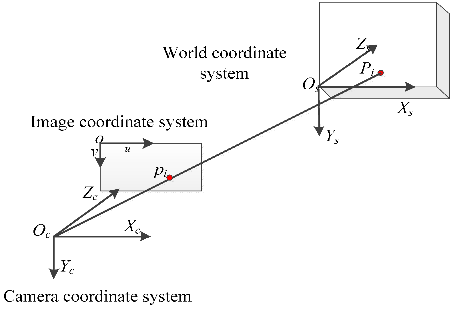
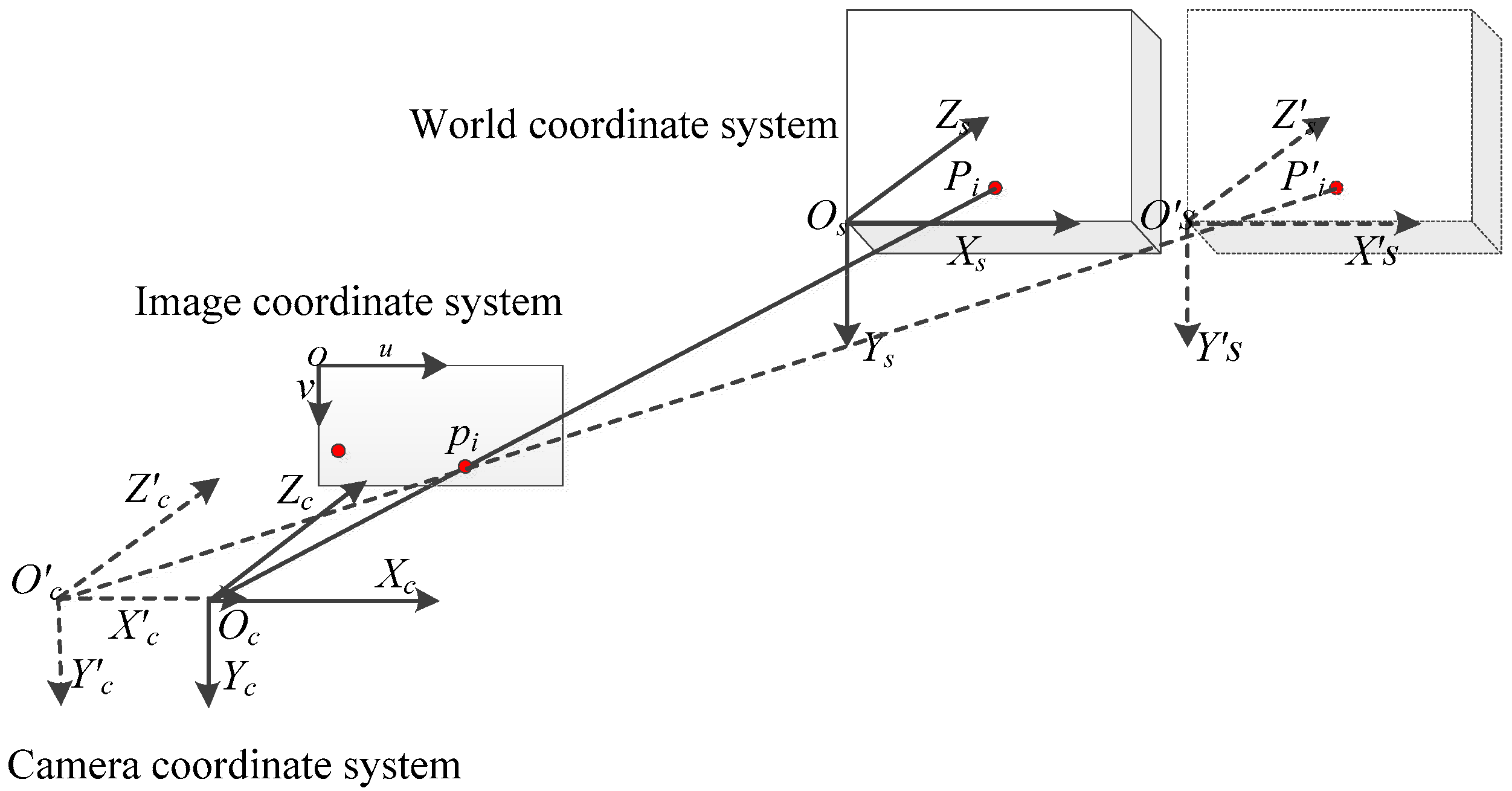
2.1. Camera Model

The camera model is shown in Figure 1. A 3D point is denoted by $P_i={\left[\begin{array}{ccc}{X}_i& Y_i& Z_i\end{array}\right]}^T$. A 2D image point is denoted by $p_i={\left[\begin{array}{cc}{u}_i& v_i\end{array}\right]}^T$. The relationship between 3D point $P_i$ and its image projection, $p_i$, is given by:

$$\begin{array}{l}{u}_i=u_0+a_x\frac{r_{11}{X}_i+r_{12}{Y}_i+r_{13}{Z}_i+t_x}{r_{31}{X}_i+r_{32}{Y}_i+r_{33}{Z}_i+t_z}\\ v_i=v_0+a_y\frac{r_{21}{X}_i+r_{22}{Y}_i+r_{23}{Z}_i+t_y}{r_{31}{X}_i+r_{32}{Y}_i+r_{33}{Z}_i+t_z}\end{array}$$

(1)

where a_x = f/d_x, a_y = f/d_y and f is the camera focal distance. In addition, d_x, d_y are pixel sizes in the horizontal and vertical directions; (u₀, v₀) is the optical center point of the image; and R, T are the rotation matrix and translation vector, respectively, which relate the world coordinate system to the camera coordinate system. Furthermore, r_ij is the i-th row and j-th column element of R, and t_x, t_y, t_z are the elements of T. For simplicity, the rotation matrix is represented by Euler angles, $\psi$, $\theta$, $\varphi$, which represent the rotation around the respective x, y and z axes.

Owing to the influence of image noise and distortion, the calibration parameters, image points and space points do not completely conform to Equation (1). Thus, we have:

$$\begin{array}{l}\mathsf{\Delta }{u}_i=u_i-u_0-a_x\frac{r_{11}X+r_{12}Y+r_{13}Z+t_x}{r_{31}X+r_{32}Y+r_{33}Z+t_z}\\ \mathsf{\Delta }{v}_i=v_i-v_0-a_y\frac{r_{21}X+r_{22}Y+r_{23}Z+t_y}{r_{31}X+r_{32}Y+r_{33}Z+t_z}\end{array}$$

(2)

$$\min f(u,v)={\displaystyle \sum _{i=1}^n(\mathsf{\Delta }{u}_i^2+\mathsf{\Delta }{v}_i^2)}$$

(3)

Equation (2) describes the calculation of image re-projection errors. Small re-projection errors are desired, which means that the calibration results satisfy Equation (3). However, the question arises of if a small image re-projection error will lead to the high calibration accuracy of the camera parameters. Analysis of the relationship between the image re-projection error and the calibration accuracy is therefore required.

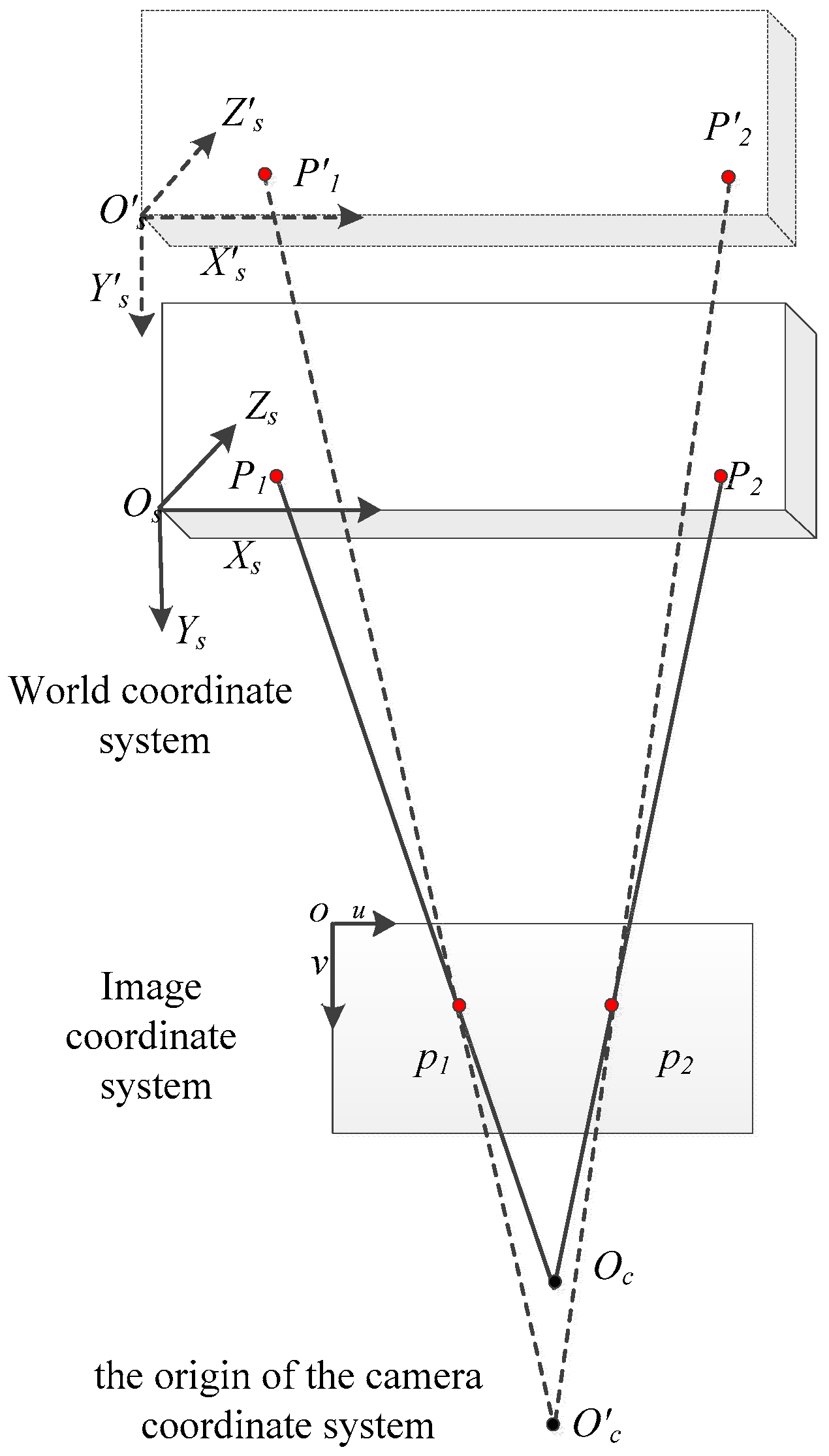
2.2. Error Coupling Analysis

The two equations in Equation (2) have the same form. We thus analyze the first equation; all conclusions can apply to the second equation. We assume that u₀ has error △u₀ and that t_x has error △t_x. From Equation (2), we have:

$$\begin{array}{c}\mathsf{\Delta }{u^{\prime }}_i=u_i-(u_0+\mathsf{\Delta }{u}_0)-a_x\frac{r_{11}{X}_i+r_{12}{Y}_i+r_{13}{Z}_i+(t_x+\mathsf{\Delta }{t}_x)}{r_{31}{X}_i+r_{32}{Y}_i+r_{33}{Z}_i+t_z}\\ =\mathsf{\Delta }{u}_i-(\mathsf{\Delta }{u}_0+\frac{\mathsf{\Delta }{t}_x{a}_x}{r_{31}{X}_i+r_{32}{Y}_i+r_{33}{Z}_i+t_z})\end{array}$$

(4)

when $\mathsf{\Delta }{t}_x=-(r_{31}{X}_i+r_{32}{Y}_i+r_{33}{Z}_i+t_z)/a_x\mathsf{\Delta }{u}_0$, we have $\mathsf{\Delta }{u^{\prime }}_i=\mathsf{\Delta }{u}_i$. The image re-projection error will not change. However, because the space point coordinate values are different, other image point re-projection errors will be changed. We assume that:

$$\begin{array}{l}\mathsf{\Delta }{t}_x=-\frac{r_{31}{X}_1+r_{32}{Y}_1+r_{33}{Z}_1+t_z}{a_x}\mathsf{\Delta }{u}_0\\ =-\frac{r_{31}{X}_i+r_{32}{Y}_i+r_{33}{Z}_i+t_z}{a_x}\mathsf{\Delta }{u}_0-\frac{r_{31}d{X}_i+r_{32}d{Y}_i+r_{33}d{Z}_i}{a_x}\mathsf{\Delta }{u}_0\end{array}$$

(5)

where dX_i = X₁ − X_i, dY_i = Y₁ − Y_i, dZ_i = Z₁ − Z_i, and image re-projection errors are given by:

$$\mathsf{\Delta }{u^{\prime }}_i=\mathsf{\Delta }{u}_i+\mathsf{\Delta }{u^{″}}_i\text{ with }\mathsf{\Delta }{u^{″}}_i=\frac{r_{31}d{X}_i+r_{32}d{Y}_i+r_{33}d{Z}_i}{r_{31}{X}_i+r_{32}{Y}_i+r_{33}{Z}_i+t_z}\mathsf{\Delta }{u}_0$$

(6)

Based on Equation (6), if $d{Z}_i$ is very small and $t_z$ is very large, the change in image re-projection errors will be very small. This is because coupling △u₀ and △t_x reduces the image re-projection error. In order to reduce the coupling effect, better results can be obtained if the 3D template is large and close to the camera. In fact, the template size is limited, and the calibration distance is limited by the field of view and the lens parameter.

With respect to focal distance and translation vector, we assume a_x has error △a_x and t_z has error △t_z. From Equation (2), we have:

$$\mathsf{\Delta }{u^{\prime }}_i=u_i-u_0-\frac{(a_x+\mathsf{\Delta }{a}_x)C_i}{B_i+\mathsf{\Delta }{t}_z}$$

(7)

where $B_i=r_{31}{X}_i+r_{32}{Y}_i+r_{33}{Z}_i$ and $C_i=r_{11}{X}_i+r_{12}{Y}_i+r_{13}{Z}_i$. We assume that $\mathsf{\Delta }{a}_x/\mathsf{\Delta }{t}_z=a_x/B_1$, and we obtain $\mathsf{\Delta }{u^{\prime }}_1=\mathsf{\Delta }{u}_1$. Other image re-projection errors are:

$$\mathsf{\Delta }{u^{\prime }}_i=\mathsf{\Delta }{u}_i+\mathsf{\Delta }{u^{″}}_i\text{ with }\mathsf{\Delta }{u^{″}}_i=-\frac{a_x{C}_i\mathsf{\Delta }{t}_z}{B_1(B_i+\mathsf{\Delta }{t}_z)}\approx -\frac{a_x{C}_i}{B_i}\times \frac{\mathsf{\Delta }{t}_z}{B_1}$$

(8)

From Equation (1), we have $a_x{C}_i/B_i\approx (u_i-u_0)$. We assume that the Euler angles of the world coordinate system relative to the camera coordinate system are zero. By setting the first space point $Z_1=1$, we have:

$$\mathsf{\Delta }{u^{″}}_i=-\frac{u_i-u_0}{t_z}\mathsf{\Delta }{t}_z$$

(9)

Based on Equation (9), if $(u_i-u_0)$ is small and $t_z$ is large, the change in the image re-projection error will be very small. This is because coupling △a_x and △t_z reduces the image re-projection error. To reduce the coupling effect, better results can be obtained if the 3D template is closer to the camera. Similar to the distortion, the camera focal distance and translation vector coupling error are related to the image point location. Therefore, under the influence of distortion, the camera focal distance and translation vector coupling error may increase the calibration error.

The coupling error is present in the geometric model. The camera model is also called a pinhole model; that is, the space point, image point and camera origin are located on the same line. Figure 2 shows the coupling between the optical center point of the image and the translation vector. When the optical center point of image O_c is offset, the origin of the camera coordinate system shifts. To continue fitting the pinhole model, the space point, P_i, under the camera coordinate system will produce an offset. The space point under the world coordinate system is fixed so that the relationship between the world coordinate system and camera coordinate system changes.

Figure 3 shows the coupling between the camera focal distance and the translation vector. The camera focal distance is calibrated based on the relative distance between multiple space points. When the camera focal distance changes, that is the origin of the camera coordinate system, O_c, moves to O'_c, the world coordinate system moves along the direction of the optical axis of the camera because the distance is fixed between P₁ and P₂. When the Euler angles are zero, the value of the optical axis direction is $t_z$.

In summary, under the influence of image noise and distortion, when the size of the templates, number of feature points and relative distance between the template and camera are certain, coupling errors occur in the camera’s intrinsic and extrinsic parameters that affect the calibration parameter accuracy. Therefore, to improve the accuracy of the calibration parameters, it is necessary to remove the parameter coupling errors.

3. Improved Direct Linear Transformation

3.1. Direct Linear Transformation

The DLT algorithm dates to the work of [4] or earlier. In [13,22], the authors analyzed the definition of the world coordinate system and proposed the use of data normalization to reduce the noise impact on the camera calibration parameters. In [10,23], the authors proposed combining the DLT algorithm with an optimization algorithm to address the camera distortion models.

The DLT algorithm consists of two steps: (1) homogeneous equation solving; and (2) parameter factorization. Space point P and its image p are related by homography M:

sp = MP with M = K[R|T]

(10)

where K is the camera intrinsic matrix. m_ij is the i-th row and j-th column element of M. The 12 parameters in M_3×4 are unknown in the matrix M'_12×1. From Equation (10), we have:

AM’ = 0 with ||M'|| = C

(11)

where C is a constant, and:

$$A=\left[\begin{array}{ccc}{P}^T& 0& -u{P}^T\\ 0& P^T& -v{P}^T\end{array}\right]A=\left[\begin{array}{ccc}{P}^T& 0& -u{P}^T\\ 0& P^T& -v{P}^T\end{array}\right]$$

(12)

Because Equation (11) is a homogeneous equation, we assume that m₃₄ is equal to one. The M matrix can be solved by singular value decomposition. We can then obtain the intrinsic and extrinsic parameters of the camera through factorization.

$$t_z=1/\sqrt{m_{31}{}^2+m_{32}{}^2+m_{33}{}^2}$$

(13)

$$u_0=t_z^2(m_{11}{m}_{31}+m_{12}{m}_{32}+m_{13}{m}_{33})$$

(14)

$$v_0=t_z^2(m_{21}{m}_{31}+m_{22}{m}_{32}+m_{23}{m}_{33})$$

(15)

$$a_x=t_z^2\sqrt{{(m_{12}{m}_{33}-m_{13}{m}_{32})}^2+{(m_{11}{m}_{33}-m_{13}{m}_{31})}^2+{(m_{11}{m}_{32}-m_{12}{m}_{31})}^2}$$

(16)

$$a_y=t_z^2\sqrt{{(m_{22}{m}_{33}-m_{23}{m}_{32})}^2+{(m_{21}{m}_{33}-m_{23}{m}_{31})}^2+{(m_{21}{m}_{32}-m_{22}{m}_{31})}^2}$$

(17)

$$t_x=t_z(m_{14}-u_0)/a_x$$

(18)

$$t_y=t_z(m_{24}-v_0)/a_y$$

(19)

$$\begin{array}{ccc}{r}_{11}=t_z(m_{11}-u_0{m}_{31})/a_x& r_{12}=t_z(m_{12}-u_0{m}_{32})/a_x& r_{13}=t_z(m_{13}-u_0{m}_{33})/a_x\\ r_{21}=t_z(m_{21}-v_0{m}_{31})/a_x& r_{22}=t_z(m_{22}-v_0{m}_{32})/a_x& r_{23}=t_z(m_{23}-v_0{m}_{33})/a_x\\ r_{31}=t_z{m}_{31}& r_{32}=t_z{m}_{32}& r_{33}=t_z{m}_{33}\end{array}$$

(20)

Accordingly, at least six non-coplanar feature points and their corresponding image points—the camera focal distance, optical center point, rotation matrix and translation vector—can be solved according to Equations (11)–(20).

However, with the influence of image noise and distortion, m_ij contains errors. From Equations (18) and (19), we have:

$$\begin{array}{l}{t}_x+\mathsf{\Delta }{t}_x=\frac{(t_z+\mathsf{\Delta }{t}_z)(m_{14}+\mathsf{\Delta }{m}_{14}-u_0-\mathsf{\Delta }{u}_0)}{a_x+\mathsf{\Delta }{a}_x}\\ t_y+\mathsf{\Delta }{t}_y=\frac{(t_z+\mathsf{\Delta }{t}_z)(m_{24}-u_0+\mathsf{\Delta }{m}_{24}-\mathsf{\Delta }{u}_0)}{a_y+\mathsf{\Delta }{a}_y}\end{array}$$

(21)

where △t_x, △t_z, △m₁₄, △t_y and △m₂₄ are errors. When $t_x\approx \frac{t_z(m_{14}-u_0)}{a_x+\mathsf{\Delta }{a}_x}$, $t_y\approx \frac{t_z(m_{24}-v_0)}{a_y+\mathsf{\Delta }{a}_y}$, we have:

$$\begin{array}{l}\Delta t_x=\frac{t_z(\Delta m_{14}-\Delta u_0)}{a_x+\Delta a_x}+\frac{\Delta t_z(m_{14}-u_0)}{a_x+\Delta a_x}+\frac{\Delta t_z(\Delta m_{14}-\Delta u_0)}{a_x+\Delta a_x}\\ \Delta t_y=\frac{t_z(\Delta m_{24}-\Delta v_0)}{a_y+\Delta a_y}+\frac{\Delta t_z(m_{24}-v_0)}{a_y+\Delta a_y}+\frac{\Delta t_z(\Delta m_{24}-\Delta v_0)}{a_y+\Delta a_y}\end{array}$$

(22)

In Equation (22), the third molecule is much smaller than the others and can be ignored. When $t_z>t_x$ and $\mathsf{\Delta }{u}_0\gg \mathsf{\Delta }{m}_{14}$, we have:

$$\mathsf{\Delta }{t}_x=-t_z\mathsf{\Delta }{u}_0/a_x$$

(23)

At the same time, when $t_z>t_y$ and $\mathsf{\Delta }{v}_0\gg \mathsf{\Delta }{m}_{24}$, we have:

$$\mathsf{\Delta }{t}_y=-t_z\mathsf{\Delta }{v}_0/a_y$$

(24)

With respect to the coupling error between the focal distance and translation vector, to simplify the analysis model, we assume that the Euler angles of the world coordinate system relative to the camera coordinate system are zero. Then, we have:

$$M=\left[\begin{array}{cccc}{a}_x/t_z& 0& u_0/t_z& (t_x{a}_x+t_z{u}_0)/t_z\\ 0& a_y/t_z& v_0/t_z& (t_y{a}_y+t_z{v}_0)/t_z\\ 0& 0& 1/t_z& 1\end{array}\right]$$

(25)

From Equation (13), we have:

$$t_z=1/m_{33}$$

(26)

From Equations (16) and (17), we have:

$$\begin{array}{l}{a}_x=t_z^2{m}_{11}{m}_{33}=m_{11}{t}_z\\ a_y=t_z^2{m}_{22}{m}_{33}=m_{22}{t}_z\end{array}$$

(27)

Owing to the influence of image noise and distortion, M contains errors. From Equation (27), we thus have:

$$\begin{array}{l}{a}_x+\mathsf{\Delta }{a}_x=m_{11}{t}_z+m_{11}\mathsf{\Delta }{t}_z+\mathsf{\Delta }{m}_{11}{t}_z+\mathsf{\Delta }{m}_{11}\mathsf{\Delta }{t}_z\\ a_y+\mathsf{\Delta }{a}_y=m_{22}{t}_z+m_{22}\mathsf{\Delta }{t}_z+\mathsf{\Delta }{m}_{22}{t}_z+\mathsf{\Delta }{m}_{22}\mathsf{\Delta }{t}_z\end{array}$$

(28)

where △a_x, △t_z, △m₁₁, △a_y and △m₂₂ are errors. $\mathsf{\Delta }{m}_{11}\mathsf{\Delta }{t}_z$ and $\mathsf{\Delta }{m}_{22}\mathsf{\Delta }{t}_z$ are much smaller than the others and can be ignored. Then, we have:

$$\begin{array}{l}\mathsf{\Delta }{a}_x=m_{11}\mathsf{\Delta }{t}_z+\mathsf{\Delta }{m}_{11}{t}_z\\ \mathsf{\Delta }{a}_y=m_{22}\mathsf{\Delta }{t}_z+\mathsf{\Delta }{m}_{22}{t}_z\end{array}$$

(29)

On account of $\mathsf{\Delta }{t}_z\gg \mathsf{\Delta }{m}_{11}$ and $\mathsf{\Delta }{t}_z\gg \mathsf{\Delta }{m}_{22}$, we have:

$$\begin{array}{l}\mathsf{\Delta }{a}_x=m_{11}\mathsf{\Delta }{t}_z\\ \mathsf{\Delta }{a}_y=m_{22}\mathsf{\Delta }{t}_z\end{array}$$

(30)

Equations (23), (24) and (30) show that a linear relationship exists between the calibration parameters after ignoring some minor errors. We use a simulation to illustrate the size of some of the ignored minor errors. In the simulation, we have a_x = 1454.5, a_y = 1454.5, u₀ = 700 pixel and v₀ = 512 pixel; moreover, the size of the pattern is 0.7 m × 0.7 m × 0.3 m. The relationship of the world coordinate system relative to the camera coordinate system relationship is represented by R = [20, 20, 20] (°) and T = [−0.25, −0.25, t_z] (mm). Gaussian noise with a zero mean and a 0.1-pixel standard deviation is added to the projected image points. The analysis of Equations (23) and (24) is shown in Figure 4. The difference between △a_x, △a_y and the results of Equations (23) and (24) is small. The analysis of Equation (30) is shown in Figure 5. Because the Euler angles are not equal to 0°, △t_x, △t_y and the result of Equation (30) are different. However, the difference is small.

Under the influence of image noise and lens distortion, the M matrix of the DLT algorithm contains errors. These errors further affect the accuracy of the calibration parameters. Through the above analysis, there is a linear coupling relationship between $\mathsf{\Delta }{t}_x$ and $\mathsf{\Delta }{u}_0$, $\mathsf{\Delta }{t}_y$ and $\mathsf{\Delta }{v}_0$, $\mathsf{\Delta }{a}_x$ and $\mathsf{\Delta }{t}_z$ and $\mathsf{\Delta }{a}_y$ and $\mathsf{\Delta }{t}_z$ after ignoring some minor errors.

3.2. Improved Direct Linear Transformation

Owing to the linear relationship that exists between the intrinsic and extrinsic parameter errors, all of these errors are unknown, and the specific error value cannot be directly solved. We assume that the 3D template only moves along the z axis. ${a^{\prime }}_x$, ${a^{\prime }}_y$, ${u^{\prime }}_0$, ${v^{\prime }}_0$, ${t^{\prime }}_x$, ${t^{\prime }}_y$ and ${t^{\prime }}_{z1}$ are calibration values of the DLT algorithm before the z axis translation. ${a^{″}}_x$, ${a^{″}}_y$, ${u^{″}}_0$, ${v^{″}}_0$, ${t^{″}}_x$, ${t^{″}}_y$ and ${t^{\prime }}_{z2}$ are calibration values of the DLT algorithm after the z axis translation. From Equations (23) and (24), we have:

$$\begin{array}{l}\mathsf{\Delta }{t^{\prime }}_x={t^{\prime }}_x-t_x=-t_{z1}({u^{\prime }}_0-u_0)/a_x\\ \mathsf{\Delta }{t^{″}}_x={t^{″}}_x-t_x=-t_{z2}({u^{″}}_0-u_0)/a_x\end{array}$$

(31)

$$\begin{array}{l}\mathsf{\Delta }{t^{\prime }}_y={t^{\prime }}_y-t_y=-t_{z1}({v^{\prime }}_0-v_0)/a_y\\ \mathsf{\Delta }{t^{″}}_y={t^{″}}_y-t_y=-t_{z2}({v^{″}}_0-v_0)/a_y\end{array}$$

(32)

where $a_x$, $a_y$, $u_0$, $v_0$, $t_x$, $t_y$, $t_{z1}$ and $t_{z2}$ are true values. Because the translation occurs only along the z axis, we set $t_{z2}=n{t}_{z1}$. From Equations (31) and (32), we have:

$$\frac{{t^{\prime }}_x-{t^{″}}_x}{n-1}=\frac{t_{z1}}{a_x}(\frac{n{u^{″}}_0-{u^{\prime }}_0}{n-1}-u_0)$$

(33)

$$\frac{{t^{\prime }}_y-{t^{″}}_y}{n-1}=\frac{t_{z1}}{a_x}(\frac{n{v^{″}}_0-{v^{\prime }}_0}{n-1}-v_0)$$

(34)

From Equation (33), a linear relationship exists between $(n{u^{″}}_0-{u^{\prime }}_0)/(n-1)$ and $({t^{\prime }}_x-{t^{″}}_x)/(n-1)$. By repeatedly moving the 3D template, $u_0$ can be solved with a linear least-squares fit. Similarly, $v_0$ can be solved by Equation (34).

From Equations (31) and (32), we have:

$$\frac{n{t^{\prime }}_x-{t^{″}}_x}{n-1}=t_x-\frac{t_z}{a_x}\frac{n({u^{″}}_0-{u^{\prime }}_0)}{n-1}$$

(35)

$$\frac{n{t^{\prime }}_y-{t^{″}}_y}{n-1}=t_y-\frac{t_z}{a_y}\frac{n({v^{″}}_0-{v^{\prime }}_0)}{n-1}$$

(36)

A linear relationship exists between $n({u^{″}}_0-{u^{\prime }}_0)/(n-1)$ and $(n{t^{\prime }}_x-{t^{″}}_x)/n-1$, $n({v^{″}}_0-{v^{\prime }}_0)/(n-1)$ and $(n{t^{\prime }}_y-{t^{″}}_y)/(n-1)$. Thus, $t_x$, $t_y$ can be solved by Equations (35) and (36).

From Equation (30), we have:

$$\begin{array}{l}{a^{\prime }}_x-a_x=(r_{11}{a}_x+r_{31}{u}_0)({t^{\prime }}_{z1}-t_{z1})/t_{z1}\\ {a^{″}}_x-a_x=(r_{11}{a}_x+r_{31}{u}_0)({t^{\prime }}_{z2}-t_{z2})/t_{z2}\end{array}$$

(37)

From Equation (37), we have:

$$(r_{11}{a}_x+r_{31}{u}_0)(({t^{\prime }}_{z2}-{t^{\prime }}_{z1})-(t_{z2}-t_{z1}))-(t_{z_2}{a^{″}}_x-t_{z_1}{a^{\prime }}_x-a_x(t_{z2}-t_{z1}))=0$$

(38)

We set $d{z}_1=t_{z2}-t_{z1}$. We then obtain:

$$(r_{11}{a}_x+r_{31}{u}_0)\frac{{t^{\prime }}_{z2}-{t^{\prime }}_{z1}-d{z}_1}{d{z}_1}-t_{z1}\frac{{a^{″}}_x-{a^{\prime }}_x}{d{z}_1}-{a^{″}}_x+a_x=0$$

(39)

Because $({a^{″}}_x-{a^{\prime }}_x)/d{z}_1$ is small, we use ${t^{\prime }}_{z1}$ to replace $t_{z1}$. Then, we have:

$$(r_{11}{a}_x+r_{31}{u}_0)\frac{{t^{\prime }}_{z2}-{t^{\prime }}_{z1}-d{z}_1}{d{z}_1}-({t^{\prime }}_{z1}\frac{{a^{″}}_x-{a^{\prime }}_x}{d{z}_1}+{a^{″}}_x)+a_x=0$$

(40)

A linear relationship exists between $({t^{\prime }}_{z2}-{t^{\prime }}_{z1}-d{z}_1)/d{z}_1$ and ${t^{\prime }}_{z1}({a^{″}}_x-{a^{\prime }}_x)/d{z}_1+{a^{″}}_x$. By repeatedly moving the 3D template, $a_x$ can be solved with a linear least-squares fit.

With respect to $t_{z1}$, from Equation (37), we have:

$$\frac{\mathsf{\Delta }{a^{\prime }}_x}{\mathsf{\Delta }{a^{″}}_x}=\frac{n({t^{\prime }}_{z_1}-t_{z_1})}{{t^{\prime }}_{z_2}-n{t}_{z_1}}$$

(41)

Then,

$$\mathsf{\Delta }{a^{\prime }}_x{t^{\prime }}_{z_2}-n\mathsf{\Delta }{a^{″}}_x{t^{\prime }}_{z_1}=t_{z_1}(n\mathsf{\Delta }{a^{\prime }}_x-n\mathsf{\Delta }{a^{″}}_x)$$

(42)

A linear relationship exists between $\mathsf{\Delta }{a^{\prime }}_x{t^{\prime }}_{z_2}-n\mathsf{\Delta }{a^{″}}_x{t^{\prime }}_{z_1}$ and $n\mathsf{\Delta }{a^{\prime }}_x-n\mathsf{\Delta }{a^{″}}_x$. By repeatedly moving the template, $t_{z1}$ can be solved with a linear least-squares fit.

For $a_y$, we have:

$$(r_{22}{a}_y+r_{32}{v}_0)\frac{{t^{\prime }}_{z2}-{t^{\prime }}_{z1}-d{z}_1}{d{z}_1}-({t^{\prime }}_{z1}\frac{{a^{″}}_y-{a^{\prime }}_y}{d{z}_1}+{a^{″}}_y)+a_y=0$$

(43)

$$\mathsf{\Delta }{a^{\prime }}_y{t^{\prime }}_{z2}-n\mathsf{\Delta }{a^{″}}_y{t^{\prime }}_{z1}=t_{z1}(n\mathsf{\Delta }{a^{\prime }}_y-n\mathsf{\Delta }{a^{″}}_y)$$

(44)

A linear relationship exists between ${t^{\prime }}_{z2}-{t^{\prime }}_{z1}-d{z}_1/d{z}_1$ and $({a^{″}}_y-{a^{\prime }}_y){t^{\prime }}_{z1}/d{z}_1+{a^{″}}_y$ and $\mathsf{\Delta }{a^{\prime }}_y{t^{\prime }}_{z2}-n\mathsf{\Delta }{a^{″}}_y{t^{\prime }}_{z1}$ and $n\mathsf{\Delta }{a^{\prime }}_y-n\mathsf{\Delta }{a^{″}}_y$. By repeatedly moving the template, $a_y$, $t_{z1}$ can be solved with a linear least-squares fit.

In sum, the 3D template along the z axis to the translation performs a DLT algorithm at each location. With the results of the DLT, $u_0$, $v_0$, $t_x$, $t_y$, $a_x$, $a_y$ and $t_{z1}$ can again be solved with a linear least-squares fit by Equations (33)–(36), (40) and (42)–(44).

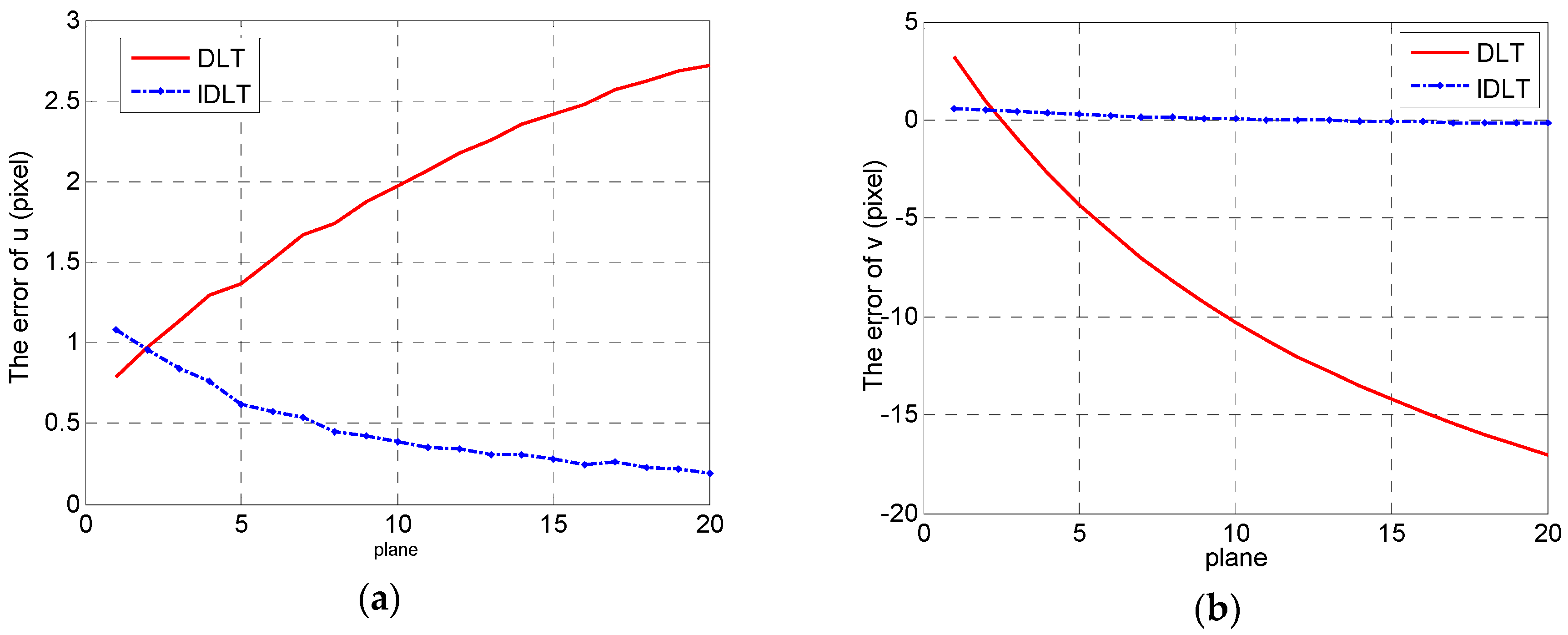
4. Experimental Section

The simulation and physical experiment parameters were set as follows. The camera focal length was 12 mm. The image resolution was 1400 × 1024. The pixel size was 7.4 μm × 7.4 μm.

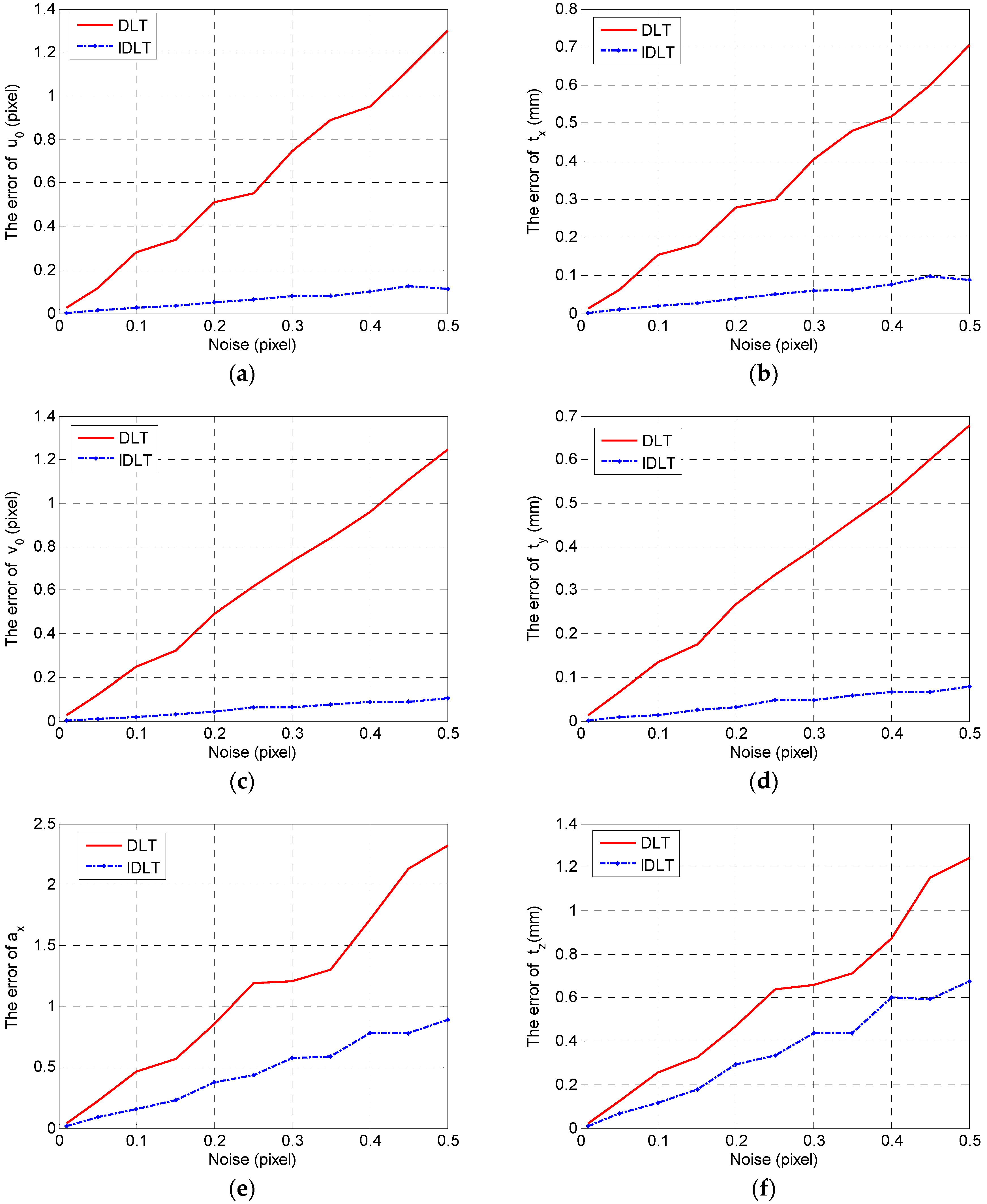
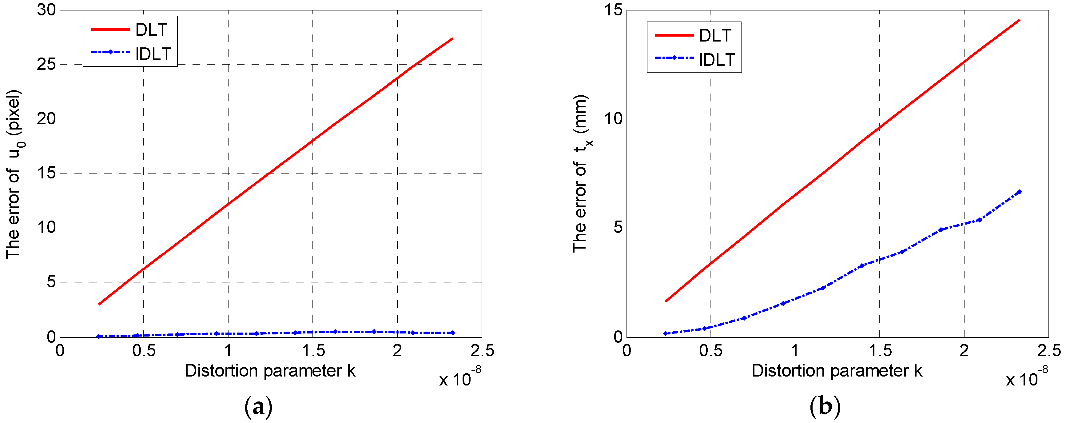
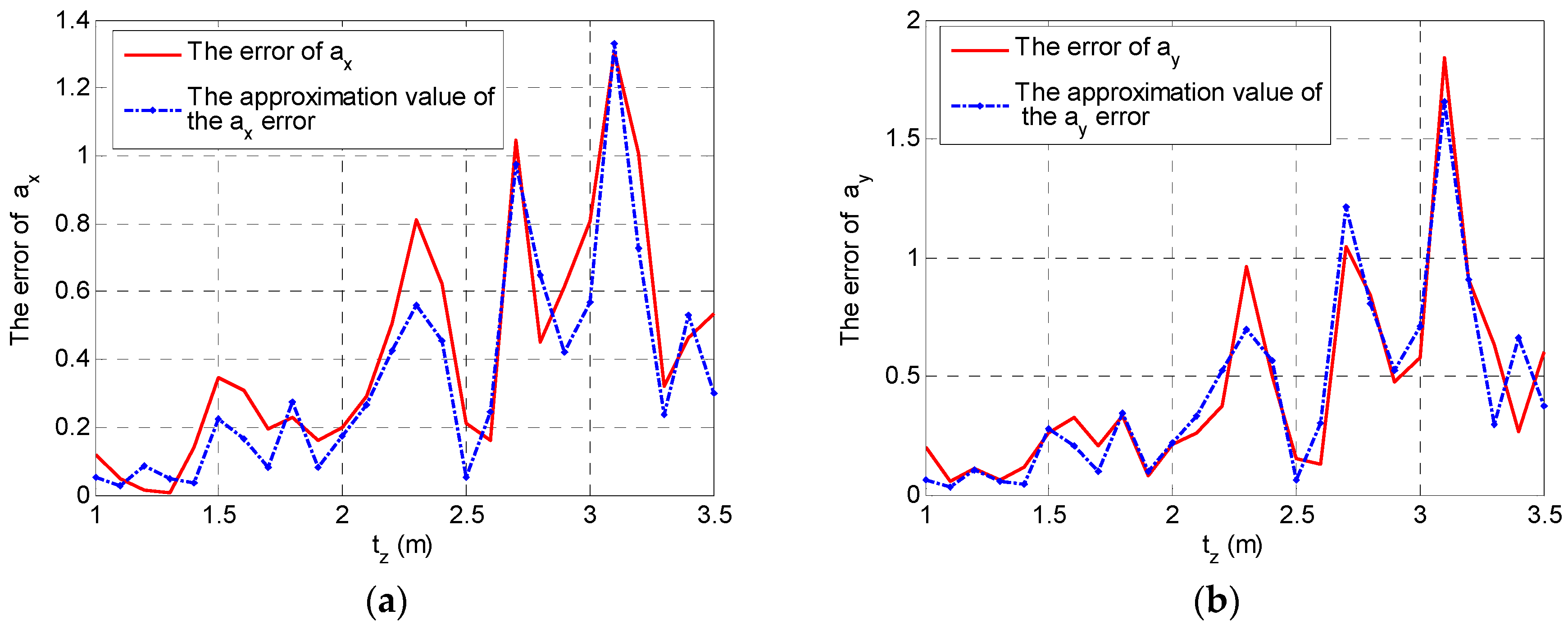
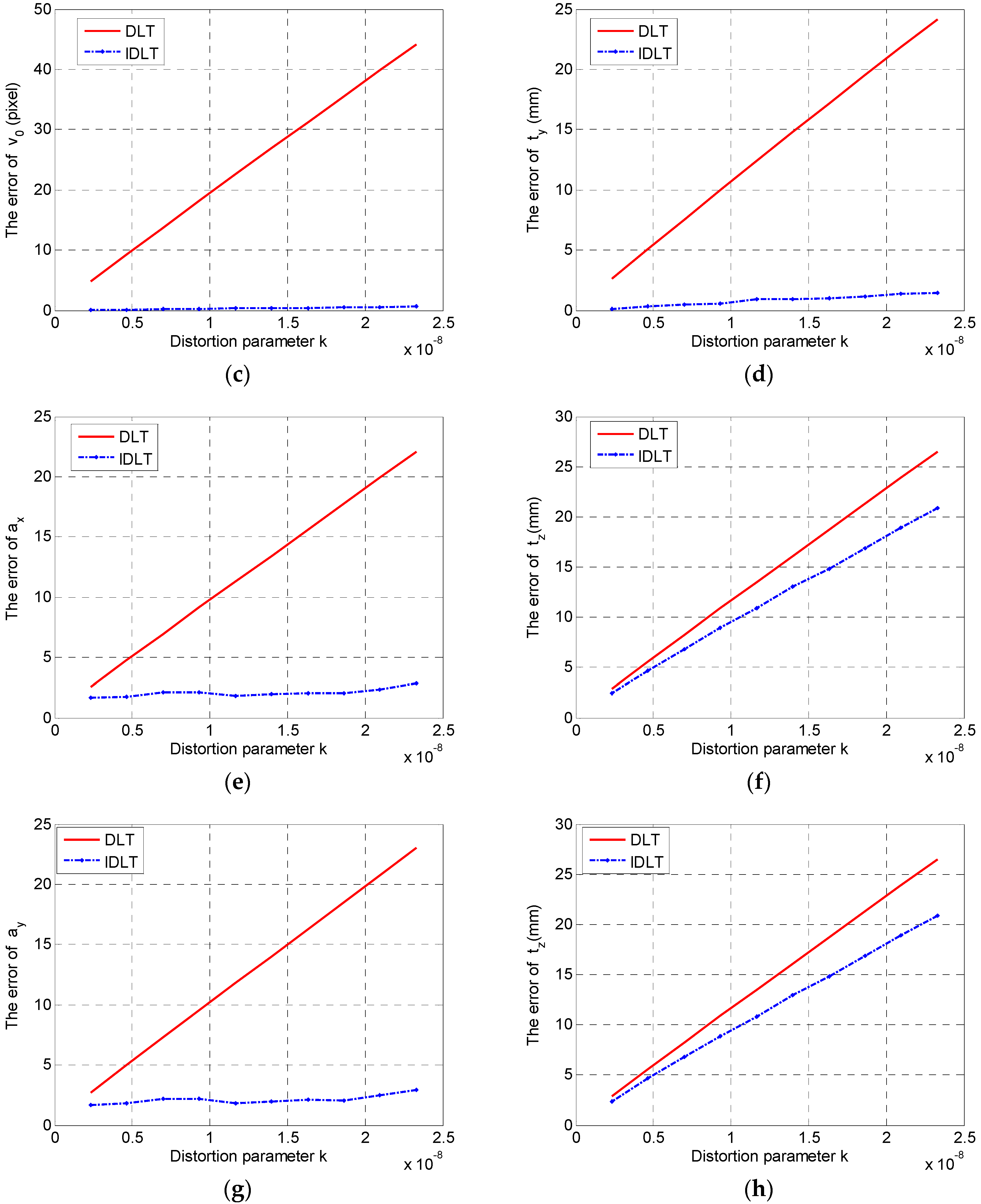
4.1. Simulation Experiment

The size of the 3D template was 0.7 m × 0.7 m × 0.3 m and contained a pattern of 8 × 8 × 3 points. The rotation matrix and translation vector were R = [10, 10, 10] (°) and T = [−0.35, −0.35, t_z] (m), t_z = 1.2–3.2 m. Gaussian noise with a 0 mean and a 0.01–0.5-pixel standard deviation was added to the projected image points. The 3D template moved 0.1 m at a time. The IDLT algorithm was calculated after 18 times of movement. A total of 100 independent tests was performed for each noise to obtain the parameter error mean and standard deviation. The error mean plus three times the standard deviation was used to represent the calibration error.

Because the calibration error became larger as t_z increased, we only analyzed the results at $t_z=1.2$m. The results of the DLT and IDLT calibration are shown in Figure 6. For $u_0$ and $v_0$, the errors of IDLT are less than 10% of the error of DLT. The errors in $t_x$ and $t_y$ are less than 0.1 mm. For $a_x$, $a_y$ and $t_z$, the errors of IDLT are less than 60% of the error of DLT.

Figure 7 shows the calibration result with noise and distortion. Gaussian noise with a 0 mean and a 0.1-pixel standard deviation is added to the projected image points. Image distortion comes from ideal image points $(u_i,v_i)$ and real image points $({u^{\prime }}_i,{v^{\prime }}_i)$ with k = 2.915 × 10⁻⁹ − 2.915 × 10⁻⁸ (the image distortion is 1–10 pixels at (1400, 0) when $u_0=700$).

$$\begin{array}{l}{u^{\prime }}_i=u_i+(u_i-u_0)k{r}^2\\ {v^{\prime }}_i=v_i+(v_i-v_0)k{r}^2\end{array}$$

(45)

Owing to the influence of image distortion, the calibration errors of DLT are relatively large. However, the calibration errors of IDLT are relatively small. In particular, the errors of $u_0$ and $v_0$ are less than 0.7 pixels, whereas the maximum error of DLT is 44 pixels. The errors of $a_x$ and $a_y$ are less than 3. Because the pixels are square, the errors of $a_x$ and $a_y$ have the same form. The error in $t_z$ is larger than that in $t_x$, $t_y$. The main reason is that $t_z$ is larger than $t_x$, $t_y$.

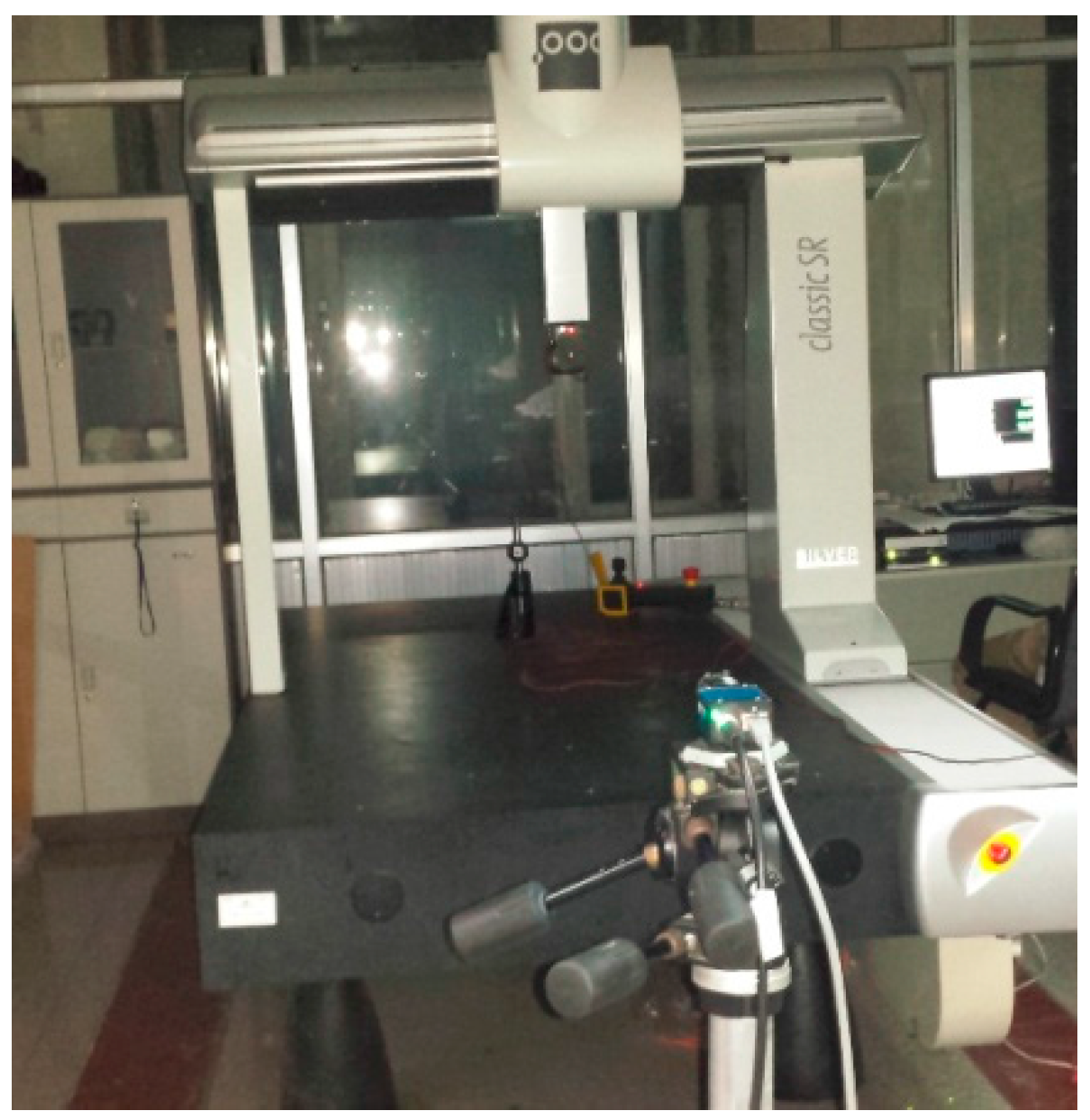
4.2. Physical Experiment

We used a light-emitting diode (LED) as the space point fixed on a coordinate measurement machine, as shown in Figure 8. The size of the plane was 0.7 m × 0.7 m, which contained a pattern of 8 × 8 points. There were 20 planes; the data for three of these planes were used for one DLT calculation. The DLT results are shown in

Table 1. DLT results of the physical experiment.

	ax	ay	u0 (pixel)	v0 (pixel)	tx (mm)	ty (mm)	tz (mm)	$\psi$ (°)	$\theta$ (°)	$\varphi$ (°)
1	1735.90	1735.56	701.09	522.07	−363.52	−319.10	1705.86	1.11	−0.13	1.36
2	1736.97	1736.67	700.97	522.59	−363.67	−317.70	1806.84	1.10	−0.13	1.36
3	1738.26	1737.96	701.66	523.22	−364.68	−316.48	1908.12	1.08	−0.13	1.36
4	1736.34	1736.05	701.59	523.46	−364.90	−314.87	2005.89	1.07	−0.13	1.36
5	1737.88	1737.58	700.65	523.91	−364.05	−313.54	2107.60	1.06	−0.13	1.36
6	1738.41	1738.15	700.71	523.93	−364.39	−311.73	2208.32	1.06	−0.12	1.36
7	1737.42	1737.20	700.71	524.02	−364.65	−310.01	2307.00	1.05	−0.12	1.36
8	1737.75	1737.60	700.58	524.17	−364.72	−308.38	2407.47	1.05	−0.12	1.36
9	1737.21	1737.07	700.71	524.16	−365.17	−306.53	2506.68	1.05	−0.13	1.36
0	1737.17	1737.05	700.54	524.10	−365.18	−304.62	2606.64	1.05	−0.12	1.35
1	1736.76	1736.63	700.66	524.31	−365.61	−303.12	2705.92	1.04	−0.12	1.35
2	1737.09	1737.00	700.74	524.76	−365.99	−302.02	2806.35	1.03	−0.13	1.35
3	1737.19	1737.11	700.97	524.85	−366.63	−300.39	2906.44	1.03	−0.13	1.35
4	1736.94	1736.86	700.96	524.60	−366.89	−298.18	3006.04	1.03	−0.13	1.36
5	1737.05	1736.98	700.83	524.52	−366.94	−296.22	3106.31	1.04	−0.13	1.36
6	1736.63	1736.56	700.75	524.32	−367.06	−294.05	3205.58	1.05	−0.13	1.35
7	1736.33	1736.27	700.88	524.43	−367.58	−292.43	3304.94	1.04	−0.13	1.35
8	1736.79	1736.77	701.40	524.66	−368.87	−291.07	3405.76	1.03	−0.14	1.35

. The fluctuations in the Euler angle errors are less than 0.06°, and they are not very volatile. The most volatile values are t_y and v₀. The fluctuation in t_y is less than 28.03 mm, and the fluctuation in v₀ is less than 2.59 pixels. The results of the IDLT algorithm are shown in

Table 2. IDLT results of the physical experiment.

ax	ay	u0 (pixel)	v0 (pixel)	tx (mm)	ty (mm)	Tz (mm)
1738.11	1738.33	696.27	555.55	−358.82	−352.39	1708.23

, where the calibration parameter values are different from those of DLT.

To compare the calibration accuracy of the two algorithms, the results of IDLT and the first set of DLT data were used to calculate the re-projection errors of 20 planes. Each plane image error was described by the mean plus three times the standard deviation of the image point re-projection errors. The results are shown in Figure 9. The calculation errors of DLT increase with the number of planes. This shows that the DLT calibration results are optimal for some planes, but not for all planes. The calibration errors of IDLT decrease with the number of planes. The reason is because the distance between the image point and optical center point of the image is small, and the effect of distortion is small.

5. Conclusions

Based on a camera model, the DLT algorithm uses linear equations to calculate the intrinsic and extrinsic camera parameters. Because the camera’s intrinsic and extrinsic parameters are simultaneously calibrated, the coupling error of the calibration parameter affects the calibration accuracy. In this paper, we analyzed the principles of intrinsic and extrinsic parameter error coupling, determined a linear coupling relationship between the intrinsic parameter calibration error and the translation vector (extrinsic parameters) calibration error and proposed the IDLT algorithm. The IDLT algorithm uses the linear coupling relationship to calculate the calibration parameters of the camera. The results of simulations and experiments show that there are significantly fewer calibration parameter errors using the IDLT algorithm than there are using DLT with noise and distortion.

References

1. Chen, I.H.; Wang, S.J. An efficient approach for dynamic calibration of multiple cameras. IEEE Trans. Autom. Sci. Eng. 2009, 6, 187–194. [Google Scholar] [CrossRef]
2. Ly, D.S.; Demonceaux, C.; Vasseur, P.; Pegard, C. Extrinsic calibration of heterogeneous cameras by line images. Mach. Vis. Appl. 2014, 25, 1601–1614. [Google Scholar] [CrossRef]
3. Peng, E.; Li, L. Camera calibration using one-dimensional information and its applications in both controlled and uncontrolled environments. Pattern Recogn. 2010, 43, 1188–1198. [Google Scholar] [CrossRef]
4. Abdel-Aziz, Y.I.; Karara, H.M. Direct linear transformation from comparator coordinates into object space coordinates in close-range photo grammetry. In Proceedings of the Symposium on Close-Range Photogrammetry, University of Illinois at Urbana-Champaign, Champaign, IL, USA, 1971; pp. 1–18.
5. Tsai, R.Y. A versatile camera calibration technique for high-accuracy 3D machine vision metrology using off-the-shelf TV cameras and lenses. IEEE J. Robot Autom 1987, 3, 323–344. [Google Scholar] [CrossRef]
6. Zhang, Z.Y. A flexible new technique for camera calibration. IEEE Trans. Pattern Anal. Mach. Intell. 2000, 22, 1330–1334. [Google Scholar] [CrossRef]
7. Chen, G.; Guo, Y.B.; Wang, H.P.; Ye, D.; Gu, Y.F. Stereo vision sensor calibration based on random spatial points given by CMM. Optik 2012, 123, 731–734. [Google Scholar] [CrossRef]
8. Samper, D.; Santolaria, J.; Brosed, F.J.; Majarena, A.C.; Aguilar, J.J. Analysis of Tsai calibration method using two- and three-dimensional calibration objects. Mach. Vis. Appl. 2013, 24, 117–131. [Google Scholar] [CrossRef]
9. Sun, W.; Cooperstock, J.R. An empirical evaluation of factors influencing camera calibration accuracy using three publicly available techniques. Mach. Vis. Appl. 2006, 17, 51–67. [Google Scholar] [CrossRef]
10. Huang, J.H.; Wang, Z.; Xue, Q.; Gao, J.M. Calibration of a camera projector measurement system and error impact analysis. Meas. Sci. Technol. 2012, 23, 125402. [Google Scholar] [CrossRef]
11. Zhou, F.Q.; Cui, Y.; Wang, Y.X.; Liu, L.; Gao, H. Accurate and robust estimation of camera parameters using RANSAC. Opt. Laser Eng. 2013, 51, 197–212. [Google Scholar] [CrossRef]
12. Ricolfe-Viala, C.; Sanchez-Salmeron, A. Camera calibration under optimal conditions. J. Opt. Soc. Am. 2011, 19, 10769–10775. [Google Scholar] [CrossRef] [PubMed]
13. Hartley, R.; Zisserman, A. Multiple View Geometry in Computer Vision; Cambridge University Press: Cambridge, UK, 2000; pp. 110–115. [Google Scholar]
14. Batista, J.; Araujo, H.; Almeida, A.T. Iterative multistep explicit camera calibration. IEEE Trans. Robot. Autom. 1999, 15, 897–917. [Google Scholar] [CrossRef]
15. Ricolfe-Viala, C.; Sanchez-Salmeron, A.; Valera, A. Efficient lens distortion correction for decoupling in calibration of wide angle lens cameras. IEEE Sens. J. 2013, 13, 854–863. [Google Scholar] [CrossRef]
16. Guillemaut, J.Y.; Aguado, A.S.; Illingworth, J. Using points at infinity for parameter decoupling in camera calibration. IEEE Trans. Pattern Anal. Mach. Intell. 2005, 27, 265–270. [Google Scholar] [CrossRef] [PubMed] [Green Version]
17. Caprile, B.; Torre, V. Using vanishing points for camera calibration. Int. J. Comput. Vis. 1990, 4, 127–140. [Google Scholar] [CrossRef]
18. He, B.W.; Zhou, X.L.; Li, Y.F. A new camera calibration method from vanishing points in a vision system. Trans. Inst. Meas. Control 2011, 33, 806–822. [Google Scholar] [CrossRef]
19. Devernay, F.; Faugeras, O. Straight lines have to be straight. Mach. Vis. Appl. 2001, 13, 14–24. [Google Scholar] [CrossRef]
20. Zhang, G.J.; He, J.J.; Yang, X.M. Calibrating camera radial distortion with cross-ratio invariability. Opt. Laser Technol. 2003, 35, 457–461. [Google Scholar] [CrossRef]
21. Li, D.D.; Wen, G.J.; Hui, B.W.; Qiu, S.H.; Wang, W.F. Cross-ratio invariant based line scan camera geometric calibration with static linear data. Opt. Laser Eng. 2014, 62, 119–125. [Google Scholar] [CrossRef]
22. Hartley, R.I. In defense of the eight-point algorithm. IEEE Trans. Pattern Anal. Mach. Intell. 1997, 19, 580–593. [Google Scholar] [CrossRef]
23. Xu, Q.Y.; Ye, D.; Chen, H.; Che, R.S.; Chen, G.; Huang, Y. A valid camera calibration based on the maximum likelihood using virtual stereo calibration pattern. In Proceedings of the International Conference on Sensing, Computing and Automation, Chongqing, China, 8–11 May 2006; pp. 2346–2351.
Figure 1. Camera model.
Algorithms 09 00031 g001
Figure 2. Relationship between the principal point and translation.
Algorithms 09 00031 g002
Figure 3. Relationship between the focal distance and translation.
Algorithms 09 00031 g003
Figure 4. Error approximate analysis: (a) t x error analysis; (b) t y error analysis.
Algorithms 09 00031 g004
Figure 5. Error approximate analysis: (a) a x error comparison; (b) a y error comparison.
Algorithms 09 00031 g005
Figure 6. Calibration error analysis between direct linear translation (DLT) and improved DLT (IDLT) with noise: (a) error of u 0 ; (b) error of v 0 ; (c) error of t x ; (d) error of t y ; (e) error of a x ; (f) error of t z based on a x ; (g) error of a y ; (h) error of t z based on a y .
Algorithms 09 00031 g006aAlgorithms 09 00031 g006b
Figure 7. Calibration error analysis between DLT and IDLT with noise and distortion: (a) error of u 0 ; (b) error of v 0 ; (c) error of t x ; (d) error of t y ; (e) error of a x ; (f) error of t z based on a x ; (g) error of a y ; (h) error of t z based on a y .
Algorithms 09 00031 g007aAlgorithms 09 00031 g007b
Figure 8. Photograph of the physical experiment.
Algorithms 09 00031 g008
Figure 9. Re-projection errors of 20 planes with DLT and IDLT calibration results: (a) u of projection image errors; (b) v of projection image errors.
Algorithms 09 00031 g009