
Co-Clustering under the Maximum Norm †

1
IGM-LabInfo, CNRS UMR 8049, Université Paris-Est Marne-la-Vallée, 77454 Marne-la-Vallée, France
2
Institut für Softwaretechnik und Theoretische Informatik, 10587 TU Berlin, Germany
*
Author to whom correspondence should be addressed.
†
This paper is an extended version of our paper published in Co-Clustering Under the Maximum Norm. In Proceedings of the 25th International Symposium on Algorithms and Computation (ISAAC’ 14), LNCS 8889, Jeonju, Korea, 15–17 December 2014; pp. 298–309.
Algorithms 2016, 9(1), 17; https://doi.org/10.3390/a9010017
Submission received: 7 December 2015
/
Revised: 10 February 2016
/
Accepted: 16 February 2016
/
Published: 25 February 2016
Abstract
:Co-clustering, that is partitioning a numerical matrix into “homogeneous” submatrices, has many applications ranging from bioinformatics to election analysis. Many interesting variants of co-clustering are NP-hard. We focus on the basic variant of co-clustering where the homogeneity of a submatrix is defined in terms of minimizing the maximum distance between two entries. In this context, we spot several NP-hard, as well as a number of relevant polynomial-time solvable special cases, thus charting the border of tractability for this challenging data clustering problem. For instance, we provide polynomial-time solvability when having to partition the rows and columns into two subsets each (meaning that one obtains four submatrices). When partitioning rows and columns into three subsets each, however, we encounter NP-hardness, even for input matrices containing only values from {0, 1, 2}.
1. Introduction
Co-clustering, also known as bi-clustering [1], performs a simultaneous clustering of the rows and columns of a data matrix. Roughly speaking, the problem is, given a numerical input matrix , to partition the rows and columns of into subsets minimizing a given cost function (measuring “homogeneity”). For a given subset I of rows and a subset J of columns, the corresponding cluster consists of all entries with and . The cost function usually defines homogeneity in terms of distances (measured in some norm) between the entries of each cluster. Note that the variant where clusters are allowed to “overlap”, meaning that some rows and columns are contained in multiple clusters, has also been studied [1]. We focus on the non-overlapping variant, which can be stated as follows.
- Co-Clustering
- Input: A matrix and two positive integers .
- Task: Find a partition of ’s rows into k subsets and a partition of ’s columns into ℓ subsets, such that a given cost function (defined with respect to some norm ) is minimized for the corresponding clustering.
Co-clustering is a fundamental paradigm for unsupervised data analysis. Its applications range from microarrays and bioinformatics over recommender systems to election analysis [1,2,3,4]. Due to its enormous practical significance, there is a vast amount of literature discussing various variants; however, due to the observed NP-hardness of “almost all interesting variants” [1], most of the literature deals with heuristic, typically empirically-validated algorithms. Indeed, there has been very active research on co-clustering in terms of heuristic algorithms, while there is little substantial theoretical work for this important clustering problem. Motivated by an effort towards a deeper theoretical analysis, as started by Anagnostopoulos et al. [2], we further refine and strengthen the theoretical investigations on the computational complexity of a natural special case of Co-Clustering, namely we study the case of being the maximum norm , where the problem comes down to minimizing the maximum distance between entries of a cluster . This cost function might be a reasonable choice in practice due to its outlier sensitivity. In network security, for example, there often exists a vast amount of “normal” data points, whereas there are only very few “malicious” data points, which are outliers with respect to certain attributes. The maximum norm does not allow one to put entries with large differences into the same cluster, which is crucial for detecting possible attacks. The maximum norm can also be applied in a discretized setting, where input values are grouped (for example, replaced by integer values) according to their level of deviation from the mean of the respective attribute. It is then not allowed to put values of different ranges of the standard deviation into the same cluster. Last, but not least, we study an even more restricted clustering version, where the partitions of the rows and columns have to contain consecutive subsets. This version subsumes the problem of feature discretization, which is used as a preprocessing technique in data mining applications [5,6,7]. See Section 3.3 for this version.
Anagnostopoulos et al. [2] provided a thorough analysis of the polynomial-time approximability of Co-Clustering (with respect to -norms), presenting several constant-factor approximation algorithms. While their algorithms are almost straightforward, relying on one-dimensionally clustering first the rows and then the columns, their main contribution lies in the sophisticated mathematical analysis of the corresponding approximation factors. Note that Jegelka et al. [8] further generalized this approach to higher dimensions, then called tensor clustering. In this work, we study (efficient) exact instead of approximate solvability. To this end, by focusing on Co-Clustering∞, we investigate a scenario that is combinatorially easier to grasp. In particular, our exact and combinatorial polynomial-time algorithms exploit structural properties of the input matrix and do not solely depend on one-dimensional approaches.
1.1. Related Work
Our main point of reference is the work of Anagnostopoulos et al. [2]. Their focus is on polynomial-time approximation algorithms, but they also provide computational hardness results. In particular, they point to challenging open questions concerning the cases , , or binary input matrices. Within our more restricted setting using the maximum norm, we can resolve parts of these questions. The survey of Madeira and Oliveira [1] (according to Google Scholar, accessed December 2015, cited more than 1500 times) provides an excellent overview on the many variations of Co-Clustering, there called bi-clustering, and discusses many applications in bioinformatics and beyond. In particular, they also discuss Hartigan’s [9] special case where the goal is to partition into uniform clusters (that is, each cluster has only one entry value). Our studies indeed generalize this very puristic scenario by not demanding completely uniform clusters (which would correspond to clusters with maximum entry difference zero), but allowing some variation between maximum and minimum cluster entries. Califano et al. [10] aim at clusterings where in each submatrix, the distance between entries within each row and within each column is upper-bounded. Recent work by Wulff et al. [11] considers a so-called “monochromatic” bi-clustering where the cost for each submatrix is defined as the number of minority entries. For binary data, this clustering task coincides with the -norm version of co-clustering, as defined by Anagnostopoulos et al. [2]. Wulff et al. [11] show the NP-hardness of monochromatic bi-clustering for binary data with an additional third value denoting missing entries (which are not considered in their cost function) and give a randomized polynomial-time approximation scheme (PTAS). Except for the work of Anagnostopoulos et al. [2] and Wulff et al. [11], all other investigations mentioned above are empirical in nature.
1.2. Our Contributions
In terms of defining “cluster homogeneity”, we focus on minimizing the maximum distance between two entries within a cluster (maximum norm). Table 1 surveys most of our results. Our main conceptual contribution is to provide a seemingly first study on the exact complexity of a natural special case of Co-Clustering, thus potentially stimulating a promising field of research.
Our main technical contributions are as follows. Concerning the computational intractability results with respect to even strongly-restricted cases, we put much effort into finding the “right” problems to reduce from in order to make the reductions as natural and expressive as possible, thus making non-obvious connections to fields, such as geometric set covering. Moreover, seemingly for the first time in the context of co-clustering, we demonstrate that the inherent NP-hardness does not stem from the permutation combinatorics behind: the problem remains NP-hard when all clusters must consist of consecutive rows or columns. This is a strong constraint (the search space size is tremendously reduced, basically from to ), which directly gives a polynomial-time algorithm for k and ℓ being constants. Note that in the general case, we have NP-hardness for constant k and ℓ. Concerning the algorithmic results, we develop a novel reduction to SAT solving (instead of the standard reductions to integer linear programming). Notably, however, as opposed to previous work on polynomial-time approximation algorithms [2,8], our methods seem to be tailored for the two-dimensional case (co-clustering), and the higher dimensional case (tensor clustering) appears to be out of reach.
2. Formal Definitions and Preliminaries
We use standard terminology for matrices. A matrix consists of m rows and n columns where denotes the entry in row i and column j. We define and for . For simplicity, we neglect the running times of arithmetical operations throughout this paper. Since we can assume that the input values of are upper-bounded polynomially in the size of (Observation 2), the blow-up in the running times is at most polynomial.
2.1. Problem Definition
We follow the terminology of Anagnostopoulos et al. [2]. For a matrix , a -co-clustering is a pair consisting of a k-partition of the row indices of (that is, for all , for all and ) and an ℓ-partition of the column indices of . We call the elements of (resp., ) row blocks (column blocks, resp.). Additionally, we require and to not contain empty sets. For , the set is called a cluster.
The cost of a co-clustering (under maximum norm, which is the only norm we consider here) is defined as the maximum difference between any two entries in any cluster , formally . Herein, () denotes the maximum (minimum, resp.) entry in .
The decision variant of Co-Clustering with maximum norm is as follows.
- Co-Clustering∞
- Input: A matrix , integers and a cost .
- Question: Is there a -co-clustering of with ?
See Figure 1 for an introductory example. We define to be the alphabet of the input matrix (consisting of the numerical values that occur in ). Note that . We use the abbreviation -Co-Clustering∞ to refer to Co-Clustering∞ with constants , and by -Co-Clustering∞, we refer to the case where only k is constant and ℓ is part of the input. Clearly, Co-Clustering∞ is symmetric with respect to k and ℓ in the sense that any -co-clustering of a matrix is equivalent to an -co-clustering of the transposed matrix . Hence, we always assume that .
We next collect some simple observations. First, determining whether there is a cost-zero (perfect) co-clustering is easy. Moreover, since, for a binary alphabet, the only interesting case is a perfect co-clustering, we get the following.
Observation 1.
Co-Clustering∞ is solvable in time for cost zero and also for any size-two alphabet.
Proof.
Let be a Co-Clustering∞ input instance. For a -co-clustering with cost zero, it holds that all entries of a cluster are equal. This is only possible if there are at most k different rows and at most ℓ different columns in , since otherwise, there will be a cluster containing two different entries. Thus, the case can be solved by lexicographically sorting the rows and columns of in time (e.g., using radix sort). ☐
We further observe that the input matrix can, without loss of generality, be assumed to contain only integer values (by some rescaling arguments preserving the distance relations between elements).
Observation 2.
For any Co-Clustering∞-instance with arbitrary alphabet , one can find in time an equivalent instance with alphabet and cost value .
Proof.
We show that for any instance with arbitrary alphabet and cost , there exists an equivalent instance with and . Let be the i-th element of Σ with respect to any fixed ordering. The idea is that the cost value c determines which elements of Σ are allowed to appear together in a cluster of a cost-c co-clustering. Namely, in any cost-c co-clustering, two elements can occur in the same cluster if and only if . These constraints can be encoded in an undirected graph with , where each vertex corresponds to an element of Σ, and there is an edge between two vertices if and only if the corresponding elements can occur in the same cluster of a cost-c co-clustering.
Now, observe that is a unit interval graph, since each vertex can be represented by the length-c interval , such that it holds (we assume all intervals to contain real values). By properly shifting and rescaling the intervals, one can find an embedding of , where the vertices are represented by length- intervals of equal integer length with integer starting points , such that , , and . Hence, replacing the elements by in the input matrix yields a matrix that has a cost- co-clustering if and only if the original input matrix has a cost-c co-clustering. Thus, for any instance with alphabet Σ and cost c, there is an equivalent instance with alphabet and cost . Consequently, we can upper-bound the values in by . ☐
Due to Observation 2, we henceforth assume for the rest of the paper that the input matrix contains integers.
2.2. Parameterized Algorithmics
We briefly introduce the relevant notions from parameterized algorithmics (refer to the monographs [12,13,14] for a detailed introduction). A parameterized problem, where each instance consists of the “classical” problem instance I and an integer ρ called parameter, is fixed-parameter tractable (FPT) if there is a computable function f and an algorithm solving any instance in time. The corresponding algorithm is called an FPT-algorithm.
3. Intractability Results
In the previous section, we observed that Co-Clustering∞ is easy to solve for binary input matrices (Observation 1). In contrast to this, we show in this section that its computational complexity significantly changes as soon as the input matrix contains at least three different entries. In fact, even for very restricted special cases, we can show NP-hardness. These special cases comprise co-clusterings with a constant number of clusters (Section 3.1) or input matrices with only two rows (Section 3.2). We also show the NP-hardness of finding co-clusterings where the row and column partitions are only allowed to contain consecutive blocks (Section 3.3).
3.1. Constant Number of Clusters
We start by showing that for input matrices containing three different entries, Co-Clustering∞ is NP-hard even if the co-clustering consists only of nine clusters.
Theorem 1.
(3, 3)-Co-Clustering∞ is NP-hard for Σ = {0, 1, 2}.
Proof.
We prove NP-hardness by reducing from the NP-complete 3-Coloring [15], where the task is to partition the vertex set of a undirected graph into three independent sets. Let be a 3-Coloring instance with and . We construct a (3, 3)-Co-Clustering∞ instance as follows. The columns of correspond to the vertices V, and the rows correspond to the edges E. For an edge with , we set and . All other matrix entries are set to 1. Hence, each row corresponding to an edge consists of 1-entries except for the columns j and , which contain 0 and 2 (see Figure 2). Thus, every co-clustering of with a cost at most puts column j and column into different column blocks. We next prove that there is a -co-clustering of with a cost at most if and only if G admits a 3-coloring.
First, assume that is a partition of the vertex set V into three independent sets. We define a ()-co-clustering of as follows. The column partition one-to-one corresponds to the three sets , that is for all . By the construction above, each row has exactly two non-1-entries being 0 and 2. We define the type of a row to be a permutation of 0, 1, 2, denoting which of the column blocks contain the 0-entry and the 2-entry. For example, a row is of type if it has a 2 in a column of and a 0 in a column of . The row partition is defined as follows: All rows of type or are put into . Rows of type or are contained in , and the remaining rows of type or are contained in . Clearly, for , it holds that the non-1-entries in any cluster are either all 0 or all 2, implying that .
Next, assume that is a ()-co-clustering of with a cost at most 1. The vertex sets , where contains the vertices corresponding to the columns in , form three independent sets: if an edge connects two vertices in , then the corresponding row would have the 0-entry and the 2-entry in the same column block , yielding a cost of 2, which is a contradiction. ☐
Theorem 1 can even be strengthened further.
Corollary 1.
Co-Clustering∞ with is NP-hard for any , even when is fixed, and the column blocks are forced to have equal sizes .
Proof.
Note that the reduction in Theorem 1 clearly holds for any . Furthermore, ℓ-Coloring with balanced partition sizes is still NP-hard for [15]. ☐
3.2. Constant Number of Rows
The reduction in the proof of Theorem 1 outputs matrices with an unbounded number of rows and columns containing only three different values. We now show that also the “dual restriction” is NP-hard, that is the input matrix only has a constant number of rows (two), but contains an unbounded number of different values. Interestingly, this special case is closely related to a two-dimensional variant of geometric set covering.
Theorem 2.
Co-Clustering∞ is NP-hard for and unbounded alphabet size .
Proof.
We give a polynomial-time reduction from the NP-complete Box Cover problem [16]. Given a set of n points in the plane and , Box Cover is the problem to decide whether there are ℓ squares , each with side length two, covering P, that is .
Let be a Box Cover instance. We define the instance as follows: The matrix has the points in P as columns. Further, we set , , . See Figure 3 for a small example.
The correctness can be seen as follows: Assume that I is a yes-instance, that is there are ℓ squares covering all points in P. We define and for all . Note that is a -co-clustering of . Moreover, since all points with indices in lie inside a square with side length two, it holds that each pair of entries in , as well as in has a distance at most two, implying .
Conversely, if is a yes-instance, then let be the -co-clustering of a cost at most two. For any , it holds that all points corresponding to the columns in Js have a pairwise distance at most two in both coordinates. Thus, there exists a square of side length two covering all of them. ☐
3.3. Clustering into Consecutive Clusters
One is tempted to assume that the hardness of the previous special cases of Co-Clustering∞ is rooted in the fact that we are allowed to choose arbitrary subsets for the corresponding row and column partitions since the problem remains hard even for a constant number of clusters and also with equal cluster sizes. Hence, in this section, we consider a restricted version of Co-Clustering∞, where the row and the column partition has to consist of consecutive blocks. Formally, for row indices with and column indices with , the corresponding consecutive -co-clustering is defined as:
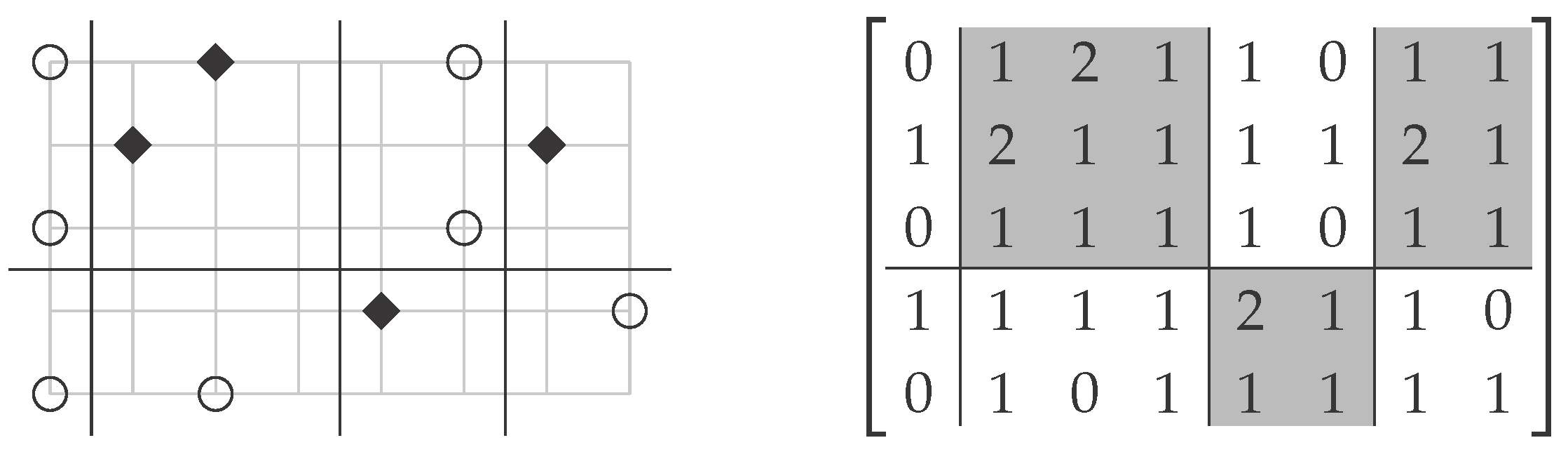
The Consecutive Co-Clustering∞ problem now is to find a consecutive -co-clustering of a given input matrix with a given cost. Again, also this restriction is not sufficient to overcome the inherent intractability of co-clustering, that is we prove it to be NP-hard. Similarly to Section 3.2, we encounter a close relation of consecutive co-clustering to a geometric problem, namely to find an optimal discretization of the plane; a preprocessing problem with applications in data mining [5,6,7]. The NP-hard Optimal Discretization problem [6] is the following: Given a set of points in the plane, where each point is either colored black (B) or white (W), and integers , decide whether there is a consistent set of k horizontal and ℓ vertical (axis-parallel) lines. That is, the vertical and horizontal lines partition the plane into rectangular regions, such that no region contains two points of different colors (see Figure 4 for an example). Here, a vertical (horizontal) line is a simple number denoting its x- (y-) coordinate.
Theorem 3.
Consecutive Co-Clustering∞ is NP-hard for Σ = {0, 1, 2}.
Proof.
We give a polynomial-time reduction from Optimal Discretization. Let be an Optimal Discretization instance; let be the set of different x-coordinates; and let be the set of different y-coordinates of the points in S. Note that n and m can be smaller than , since two points can have the same x- or y-coordinate. Furthermore, assume that and . We now define the Consecutive Co-Clustering∞ instance as follows: The matrix has columns labeled with and rows labeled with . For , the entry is defined as zero if , two if and otherwise one. The cost is set to . Clearly, this instance can be constructed in polynomial time.
To verify the correctness of the reduction, assume first that I is a yes-instance, that is there is a set of k horizontal lines and a set of ℓ vertical lines partitioning the plane consistently. We define row indices , and column indices , . For the corresponding -co-clustering , it holds that no cluster contains both values zero and two, since otherwise the corresponding partition of the plane defined by H and V contains a region with two points of different colors, which contradicts consistency. Thus, we have , implying that is a yes-instance.
Conversely, if is a yes-instance, then there exists a -co-clustering with cost at most one, that is no cluster contains both values zero and two. Clearly, then, the k horizontal lines , , and the ℓ vertical lines , are consistent. Hence, I is a yes-instance. ☐
Note that even though Consecutive Co-Clustering∞ is NP-hard, there still is some difference in its computational complexity compared to the general version. In contrast to Co-Clustering∞, the consecutive version is polynomial-time solvable for constants k and ℓ by simply trying out all consecutive partitions of the rows and columns.
4. Tractability Results
In Section 3, we showed that Co-Clustering∞ is NP-hard for and also for in the case of unbounded ℓ and . In contrast to these hardness results, we now investigate which parameter combinations yield tractable cases. It turns out (Section 4.2) that the problem is polynomial-time solvable for and for . We can even solve the case and for in polynomial time by showing that this case is in fact equivalent to the case . Note that these tractability results nicely complement the hardness results from Section 3. We further show fixed-parameter tractability for the parameters size of the alphabet and the number of column blocks ℓ (Section 4.3).
We start (Section 4.1) by describing a reduction of Co-Clustering∞ to CNF-SAT (the satisfiability problem for Boolean formulas in conjunctive normal form). Later on, it will be used in some special cases (see Theorems 5 and 7), because there, the corresponding formula, or an equivalent formula, only consists of clauses containing two literals, thus being a polynomial-time solvable 2-SAT instance.
4.1. Reduction to CNF-SAT Solving
In this section, we describe two approaches to solve Co-Clustering∞ via CNF-SAT. The first approach is based on a straightforward reduction of a Co-Clustering∞ instance to one CNF-SAT instance with clauses of size at least four. Note that this does not yield any theoretical improvements in general. Hence, we develop a second approach, which requires solving many CNF-SAT instances with clauses of size at most . The theoretical advantage of this approach is that if k and ℓ are constants, then there are only polynomially many CNF-SAT instances to solve. Moreover, the formulas contain smaller clauses (for , we even obtain polynomial-time solvable 2-SAT instances). While the second approach leads to (theoretically) tractable special cases, it is not clear that it also performs better in practice. This is why we conducted some experiments for empirical comparison of the two approaches (in fact, it turns out that the straightforward approach allows one to solve larger instances). In the following, we describe the reductions in detail and briefly discuss the experimental results.
We start with the straightforward polynomial-time reduction from Co-Clustering∞ to CNF-SAT. We simply introduce a variable () for each pair of row index and row block index (respectively, column index and column block index ) denoting whether the respective row (column) may be put into the respective row (column) block. For each row i, we enforce that it is put into at least one row block with the clause (analogously for the columns). We encode the cost constraints by introducing clauses , for each pair of entries with . These clauses simply ensure that and are not put into the same cluster. Note that this reduction yields a CNF-SAT instance with variables and clauses of size up to .
Based on experiments (using the PicoSAT Solver of Biere [17]), which we conducted on randomly generated synthetic data (of size up to ), as well as on a real-world dataset (animals with attributes dataset [18] with and ), we found that we can solve instances up to using the above CNF-SAT approach. In our experiments, we first computed an upper and a lower bound on the optimal cost value c and then created the CNF-SAT instances for decreasing values for c, starting from the upper bound. The upper and the lower bound have been obtained as follows: Given a -Co-Clustering∞ instance on , solve -Co-Clustering∞ and -Co-Clustering∞ separately for input matrix . Let and denote the - and -co-clustering, respectively, and let their costs be and . We take as a lower bound and as an upper bound on the optimal cost value for an optimal ()-co-clustering of . It is straightforward to argue the correctness of the lower bound, and we next show that is an upper bound. Consider any pair , such that i and are in the same row block of , and j and are in the same column block of (that is, and are in the same cluster). Then, it holds . Hence, just taking the row partitions from and the column partitions from gives a combined ()-co-clustering of cost at most .
From a theoretical perspective, the above naive approach of solving Co-Clustering∞ via CNF-SAT does not yield any improvement in terms of polynomial-time solvability. Therefore, we now describe a different approach, which leads to some polynomial-time solvable special cases. To this end, we introduce the concept of cluster boundaries, which are basically lower and upper bounds for the values in a cluster of a co-clustering. Formally, given two integers , an alphabet Σ and a cost c, we define a cluster boundary to be a matrix . We say that a -co-clustering of satisfies a cluster boundary if for all . It can easily be seen that a given -co-clustering has cost at most c if and only if it satisfies at least one cluster boundary , namely the one with .
The following “subtask” of Co-Clustering∞ can be reduced to a certain CNF-SAT instance: Given a cluster boundary and a Co-Clustering∞ instance I, find a co-clustering for I that satisfies . The polynomial-time reduction provided by the following lemma can be used to obtain exact Co-Clustering∞ solutions with the help of SAT solvers, and we use it in our subsequent algorithms.
Lemma 1.
Given a Co-Clustering∞-instance and a cluster boundary , one can construct in polynomial time a CNF-SAT instance φ with at most variables per clause, such that φ is satisfiable if and only if there is a ()-co-clustering of , which satisfies .
Proof.
Given an instance of Co-Clustering∞ and a cluster boundary , we define the following Boolean variables: For each , the variable represents the expression “row i could be put into row block ”. Similarly, for each , the variable represents that “column j could be put into column block ”.
We now define a Boolean CNF formula containing the following clauses: a clause for each row and a clause for each column . Additionally, for each and each , such that element does not fit into the cluster boundary at coordinate , that is , there is a clause ). Note that the clauses and ensure that row i and column j are put into some row and some column block, respectively. The clause expresses that it is impossible to have both row i in block and column j in block if does not satisfy . Clearly, is satisfiable if and only if there exists a ()-co-clustering of satisfying the cluster boundary . Note that consists of variables and clauses. ☐
Using Lemma 1, we can solve Co-Clustering∞ by solving many CNF-SAT instances (one for each possible cluster boundary) with variables and clauses of size at most . We also implemented this approach for comparison with the straightforward reduction to CNF-SAT above. The bottleneck of this approach, however, is the number of possible cluster boundaries, which grows extremely quickly. While a single CNF-SAT instance can be solved quickly, generating all possible cluster boundaries together with the corresponding CNF formulas becomes quite expensive, such that we could only solve instances with very small values of and .
4.2. Polynomial-Time Solvability
We first present a simple and efficient algorithm for -Co-Clustering∞, that is the variant where all rows belong to one row block.
Theorem 4.
-Co-Clustering∞ is solvable in time.
Proof.
We show that Algorithm 1 solves -Co-Clustering∞. In fact, it even computes the minimum , such that has a -co-clustering of cost c. The overall idea is that with only one row block all entries of a column j are contained in a cluster in any solution, and thus, it suffices to consider only the minimum and the maximum value in column j. More precisely, for a column block of a solution, it follows that . The algorithm starts with the column that contains the overall minimum value of the input matrix, that is . Clearly, has to be contained in some column block, say . The algorithm then adds all other columns j to where , removes the columns from the matrix and recursively proceeds with the column containing the minimum value of the remaining matrix. We continue with the correctness of the described procedure.
| Algorithm 1: Algorithm for (1, ∗)-Co-Clustering∞. |
| Input: , , . |
| Output: A partition of [n] into at most ℓ blocks yielding a cost of at most c, or no if no such partition exists. |
 |
If Algorithm 1 returns at Line 12, then this is a column partition into blocks satisfying the cost constraint. First, it is a partition by construction: the sets are successively removed from until it is empty. Now, let . Then, for all , it holds (by definition of ) and (by definition of ). Thus, holds for all , which yields cost∞.
Otherwise, if Algorithm 1 returns no in Line 5, then it is clearly a no-instance, since the difference between the maximum and the minimum value in a column is larger than c. If no is returned in Line 13, then the algorithm has computed column indices and column blocks for each , and there still exists at least one index in when the algorithm terminates. We claim that the columns all have to be in different blocks in any solution. To see this, consider any with . By construction, . Therefore, holds, and columns and contain elements with distance more than c. Thus, in any co-clustering with cost at most c, columns must be in different blocks, which is impossible with only ℓ blocks. Hence, we indeed have a no-instance.
The time complexity is seen as follows. The first loop examines in time all elements of the matrix. The second loop can be performed in time if the and the are sorted beforehand, requiring time. Overall, the running time is in . ☐
From now on, we focus on the case, that is we need to partition the rows into two blocks. We first consider the simplest case, where also .
Theorem 5.
(2, 2)-Co-Clustering∞ is solvable in time.
Proof.
We use the reduction to CNF-SAT provided by Lemma 1. First, note that a cluster boundary can only be satisfied if it contains the elements and . The algorithm enumerates all of these cluster boundaries. For a fixed , we construct the Boolean formula . Observe that this formula is in two-CNF form: The formula consists of k-clauses, ℓ-clauses and 2-clauses, and we have . Hence, we can determine whether it is satisfiable in linear time [19] (note that the size of the formula is in ). Overall, the input is a yes-instance if and only if is satisfiable for some cluster boundary . ☐
Finally, we show that it is possible to extend the above result to any number of column blocks for size-three alphabets.
Theorem 6.
(2, ∗)-Co-Clustering∞ is -time solvable for .
Proof.
Let be a (2, ∗)-Co-Clustering∞ instance. We assume without loss of generality that . The case is solvable in time by Theorem 5. Hence, it remains to consider the case . As , there are four potential values for a minimum-cost ()-co-clustering. Namely, cost zero (all cluster entries are equal), cost , cost and cost . Since any ()-co-clustering is of cost at most and because it can be checked in time whether there is a ()-co-clustering of cost zero (Observation 1), it remains to check whether there is a ()-co-clustering between these two extreme cases, that is for .
Avoiding a pair means to find a co-clustering without a cluster containing x and y. If (Case 1), then the problem comes down to finding a ()-co-clustering avoiding the pair . Otherwise (Case 2), the problem is to find a ()-co-clustering avoiding the pair and, additionally, either or .
Case 1.
Finding a ()-co-clustering avoiding :
In this case, we substitute , and . We describe an algorithm for finding a ()-co-clustering of cost one (avoiding ). We assume that there is no ()-co-clustering of cost one (iterating over all values from two to ℓ). Consider a ()-co-clustering of cost one, that is for all , it holds or . For , let denote the ()-co-clustering where the column blocks and are merged. By assumption, for all , it holds that , since otherwise, we have found a ()-co-clustering of cost one. It follows that or holds for all . This can only be true for .
This proves that there is a ()-co-clustering of cost one if and only if there is a ()-co-clustering of cost one. Hence, Theorem 5 shows that this case is -time solvable.
Case 2.
Finding a ()-co-clustering avoiding and (or ):
In this case, we substitute , and if has to be avoided, or if has to be avoided. It remains to determine whether there is a ()-co-clustering with cost zero, which can be done in time due to Observation 1. ☐
4.3. Fixed-Parameter Tractability
We develop an algorithm solving -Co-Clustering∞ for based on our reduction to CNF-SAT (see Lemma 1). The main idea is, given matrix and cluster boundary , to simplify the Boolean formula into a 2-Sat formula, which can be solved efficiently. This is made possible by the constraint on the cost, which imposes a very specific structure on the cluster boundary. This approach requires to enumerate all (exponentially many) possible cluster boundaries, but yields fixed-parameter tractability for the combined parameter .
Theorem 7.
-Co-Clustering∞ is -time solvable for .
In the following, we prove Theorem 7 in several steps.
A first sub-result for the proof of Theorem 7 is the following lemma, which we use to solve the case where the number of possible row partitions is less than .
Lemma 2.
For a fixed row partition I, one can solve Co-Clustering∞ in time. Moreover, Co-Clustering∞ is fixed-parameter tractable with respect to the combined parameter ().
Proof.
Given a fixed row partition , the algorithm enumerates all different cluster boundaries . We say that a given column j fits in column block if, for each and , we have (this can be decided in time for any pair ). The input is a yes-instance if and only if for some cluster boundary , every column fits in at least one column block.
Fixed-parameter tractability with respect to is obtained from two simple further observations. First, all possible row partitions can be enumerated in time. Second, since each of the clusters contains at most different values, the alphabet size for yes-instances is upper-bounded by . ☐
The following lemma, also used for the proof of Theorem 7, yields that even for the most difficult instances, there is no need to consider more than two column clusters to which any column can be assigned.
Lemma 3.
Let be an instance of -Co-Clustering∞, be an integer, , and be a cluster boundary with pairwise different columns, such that for all .
Then, for any column , two indices and can be computed in time , such that if I has a solution satisfying with , then it has one where each column j is assigned to either or .
Proof.
We write ( for any solution with ). Given a column and any element , we write for the number of entries with value a in column j.
Consider a column block , . Write for the three values, such that , and . Note that . We say that column j fits into column block if the following three conditions hold:
- for any ,
- and
- .
Note that if Condition (1) is violated, then the column contains an element that is neither in nor in . If Condition (2) (respectively Condition (3)) is violated, then there are more than (respectively ) rows that have to be in row block (respectively ). Thus, if j does not fit into a column block , then there is no solution where . We now need to find out, for each column, to which fitting column blocks it should be assigned.
Intuitively, we now prove that in most cases, a column has at most two fitting column blocks and, in the remaining cases, at most two pairs of “equivalent” column blocks.
Consider a given column . Write and . If , then Condition (1) is always violated: j does not fit into any column block, and the instance is a no-instance. If , then, again, by Condition (1), j can only fit into a column block where . There are at most two such column blocks: we write and for their indices ( if a single column block fits). The other easy case is when , i.e., all values in column j are equal to a. If j fits into column block , then, with Conditions (2) and (3), , and is one of the at most two column blocks having : again, we write and for their indices.
Finally, consider a column j with , and let be such that j fits into . Then, by Condition (1), the “middle-value” for column block is . The pair must be from . We write for the four column blocks (if they exist) corresponding to these four cases. We define if j fits into , and otherwise. Similarly, we define if j fits into , and otherwise.
Consider a solution assigning j to , with . Since j must fit into , the only possibility is that and . Thus, j fits into both and , so Conditions (2) and (3) imply and . Since , we have and . Thus, placing j in either column block yields the same row partition, namely and . Hence, the solution assigning j to , can assign it to , instead, without any further need for modification.
Similarly, with and , any solution assigning j to or can assign it to without any other modification. Thus, since any solution must assign j to one of , it can assign it to one of instead. ☐
We now give the proof of Theorem 7.
Proof.
Let be a -Co-Clustering∞ instance. The proof is by induction on ℓ. For , the problem is solvable in time (Theorem 4). We now consider general values of ℓ. Note that if ℓ is large compared to m (that is, ), then one can directly guess the row partition and run the algorithm of Lemma 2. Thus, for the running time bound, we now assume that . By Observation 2, we can assume that .
Given a ()-co-clustering , a cluster boundary satisfied by , and , each column block is said to be:
- with equal bounds if ,
- with non-overlapping bounds if ,
- with properly overlapping bounds otherwise.
We first show that instances implying a solution containing at least one column block with equal or non-overlapping bounds can easily be dealt with.
Claim 1.
If the solution contains a column-block with equal bounds, then it can be computed in time.
Proof.
Assume, without loss of generality, that the last column block, , has equal bounds. We try all possible values of . Note that column block imposes no restrictions on the row partition. Hence, it can be determined independently of the rest of the co-clustering. More precisely, any column with all values in can be put into this block, and all other columns have to end up in the other blocks, thus forming an instance of -Co-Clustering∞. By induction, each of these cases can be tested in time. Since we test all values of u, this procedure finds a solution with a column block having equal bounds in time. ☐
Claim 2.
If the solution contains a (non-empty) column-block with non-overlapping bounds, then it can be computed in time.
Proof.
Write s for the index of the column block with non-overlapping bounds, and assume that, without loss of generality, . We try all possible values of , and we examine each column . We remark that the row partition is entirely determined by column j if it belongs to column block . That is, if , then and . Using the algorithm described in Lemma 2, we deduce the column partition in time, which is bounded by . ☐
We can now safely assume that the solution contains only column blocks with properly overlapping bounds. In a first step, we guess the values of the cluster boundary . Note that, for each , we only need to consider the cases where , that is, for , we have . Note also that, for any two distinct column blocks and , we have or . We then enumerate all possible values of (the height of the first row block), and we write . Overall, there are at most cases to consider.
Using Lemma 3, we compute integers for each column j, such that any solution satisfying the above conditions (cluster boundary and ) can be assumed to assign each column j to one of or .
We now introduce a 2-Sat formula allowing us to simultaneously assign the rows and columns to the possible blocks. Let be the formula as provided by Lemma 1. Create a formula from where, for each column , the column clause is replaced by the smaller clause . Note that is a 2-Sat formula, since all other clauses or already contain at most two literals.
If is satisfiable, then is satisfiable, and admits a ()-co-clustering satisfying . Conversely, if admits a ()-co-clustering satisfying with , then, by the discussion above, there exists a co-clustering where each column j is in one of the column blocks or . In the corresponding Boolean assignment, each clause of is satisfied and each new column clause of is also satisfied. Hence, is satisfiable. Overall, for each cluster boundary and each , we construct and solve the formula defined above. The matrix admits a ()-co-clustering of cost one if and only if is satisfiable for some and .
The running time for constructing and solving the formula , for any fixed cluster boundary and any height , is in , which gives a running time of for this last part. Overall, the running time is thus . ☐
Finally, we obtain the following simple corollary.
Corollary 2.
(2, ∗)-Co-Clustering∞ with is fixed-parameter tractable with respect to parameter and with respect to parameter ℓ.
Proof.
Theorem 7 presents an FPT-algorithm with respect to the combined parameter . For -Co-Clustering∞ with , both parameters can be polynomially upper-bounded within each other. Indeed, (otherwise, there are two column blocks with identical cluster boundaries, which could be merged) and (each column block may contain two intervals, each covering at most elements). ☐
5. Conclusions
Contrasting previous theoretical work on polynomial-time approximation algorithms [2,8], we started to closely investigate the time complexity of exactly solving the NP-hard Co-Clustering∞ problem, contributing a detailed view of its computational complexity landscape. Refer to Table 1 for an overview on most of our results.
Several open questions derive from our work. Perhaps the most pressing open question is whether the case and is polynomial-time solvable or NP-hard in general. So far, we only know that (2, ∗)-Co-Clustering∞ is polynomial-time solvable for ternary matrices (Theorem 6). Another open question is the computational complexity of higher-dimensional co-clustering versions, e.g., on three-dimensional tensors as input (the most basic case here corresponds to (2,2,2)-Co-Clustering∞, that is partitioning each dimension into two subsets). Indeed, other than the techniques for deriving approximation algorithms [2,8], our exact methods do not seem to generalize to higher dimensions. Last, but not least, we do not know whether Consecutive Co-Clustering∞ is fixed-parameter tractable or W[1]-hard with respect to the combined parameter .
We conclude with the following more abstract vision on future research: Note that for the maximum norm, the cost value c defines a “conflict relation” on the values occurring in the input matrix. That is, for any two numbers with , we know that they must end up in different clusters. These conflict pairs completely determine all constraints of a solution, since all other pairs can be grouped arbitrarily. This observation can be generalized to a graph model. Given a “conflict relation” determining which pairs are not allowed to be put together into a cluster, we can define the “conflict graph” . Studying co-clusterings in the context of such conflict graphs and their structural properties could be a promising and fruitful direction for future research.
Acknowledgments
Laurent Bulteau: Main work done while affiliated with TU Berlin, supported by the Alexander von Humboldt Foundation, Bonn, Germany. Vincent Froese: Supported by the DFG, project DAMM (NI 369/13). We thank Stéphane Vialette (Université Paris-Est Marne-la-Vallée) for stimulating discussions.
Author Contributions
Laurent Bulteau, Vincent Froese, Sepp Hartung and Rolf Niedermeier drafted, wrote and revised the paper. Laurent Bulteau, Vincent Froese, Sepp Hartung and Rolf Niedermeier conceived and designed experiments. Vincent Froese conducted experiments.
Conflicts of Interest
The authors declare no conflict of interest.
References
- Madeira, S.C.; Oliveira, A.L. Biclustering Algorithms for Biological Data Analysis: A Survey. IEEE/ACM Trans. Comput. Biol. Bioinf. 2004, 1, 24–45. [Google Scholar] [CrossRef] [PubMed]
- Anagnostopoulos, A.; Dasgupta, A.; Kumar, R. A Constant-Factor Approximation Algorithm for Co-clustering. Theory Comput. 2012, 8, 597–622. [Google Scholar] [CrossRef]
- Banerjee, A.; Dhillon, I.S.; Ghosh, J.; Merugu, S.; Modha, D.S. A Generalized Maximum Entropy Approach to Bregman Co-clustering and Matrix Approximation. J. Mach. Learn. Res. 2007, 8, 1919–1986. [Google Scholar]
- Tanay, A.; Sharan, R.; Shamir, R. Biclustering Algorithms: A Survey. In Handbook of Computational Molecular Biology; Chapman & Hall/CRC: Boca Raton, FL, USA, 2005. [Google Scholar]
- Nguyen, S.H.; Skowron, A. Quantization Of Real Value Attributes-Rough Set and Boolean Reasoning Approach. In Proceedings of the Second Joint Annual Conference on Information Sciences, Wrightsville Beach, NC, USA, 28 September–1 October 1995; pp. 34–37.
- Chlebus, B.S.; Nguyen, S.H. On Finding Optimal Discretizations for Two Attributes. In Proceedings of the First International Conference on Rough Sets and Current Trends in Computing (RSCTC’98), Warsaw, Poland, 22–26 June 1998; pp. 537–544.
- Nguyen, H.S. Approximate Boolean Reasoning: Foundations and Applications in Data Mining. In Transactions on Rough Sets V; Springer: Berlin Heidelberg, Germany, 2006; pp. 334–506. [Google Scholar]
- Jegelka, S.; Sra, S.; Banerjee, A. Approximation Algorithms for Tensor Clustering. In Proceedings of the 20th International Conference of Algorithmic Learning Theory (ALT’09), Porto, Portugal, 3–5 October 2009; pp. 368–383.
- Hartigan, J.A. Direct clustering of a data matrix. J. Am. Stat. Assoc. 1972, 67, 123–129. [Google Scholar] [CrossRef]
- Califano, A.; Stolovitzky, G.; Tu, Y. Analysis of Gene Expression Microarrays for Phenotype Classification. In Proceedings of the Eighth International Conference on Intelligent Systems for Molecular Biology (ISMB’00), AAAI, San Diego, CA, USA, 16–23 August 2000; pp. 75–85.
- Wulff, S.; Urner, R.; Ben-David, S. Monochromatic Bi-Clustering. In Proceedings of the 30th International Conference on Machine Learning (ICML’13), Atlanta, GA, USA, 16–21 June 2013; pp. 145–153.
- Cygan, M.; Fomin, F.V.; Kowalik, Ł.; Lokshtanov, D.; Marx, D.; Pilipczuk, M.; Pilipczuk, M.; Saurabh, S. Parameterized Algorithms; Springer International Publishing: Switzerland, 2015. [Google Scholar]
- Downey, R.G.; Fellows, M.R. Fundamentals of Parameterized Complexity; Springer: London, UK, 2013. [Google Scholar]
- Niedermeier, R. Invitation to Fixed-Parameter Algorithms; Oxford University Press: Oxford, UK, 2006. [Google Scholar]
- Garey, M.R.; Johnson, D.S. Computers and Intractability: A Guide to the Theory of NP-Completeness; W. H. Freeman and Company: New York, NY, USA, 1979. [Google Scholar]
- Fowler, R.J.; Paterson, M.S.; Tanimoto, S.L. Optimal Packing and Covering in the Plane are NP-Complete. Inf. Process. Lett. 1981, 12, 133–137. [Google Scholar] [CrossRef]
- Biere, A. PicoSAT Essentials. J. Satisf. Boolean Model. Comput. 2008, 4, 75–97. [Google Scholar]
- Lampert, C.H.; Nickisch, H.; Harmeling, S. Attribute-Based Classification for Zero-Shot Visual Object Categorization. IEEE Trans. Pattern Anal. Mach. Intell. 2013, 36, 453–465. [Google Scholar] [CrossRef] [PubMed]
- Aspvall, B.; Plass, M.F.; Tarjan, R.E. A Linear-Time Algorithm for Testing the Truth of Certain Quantified Boolean Formulas. Inf. Process. Lett. 1979, 8, 121–123. [Google Scholar] [CrossRef]
Figure 1.
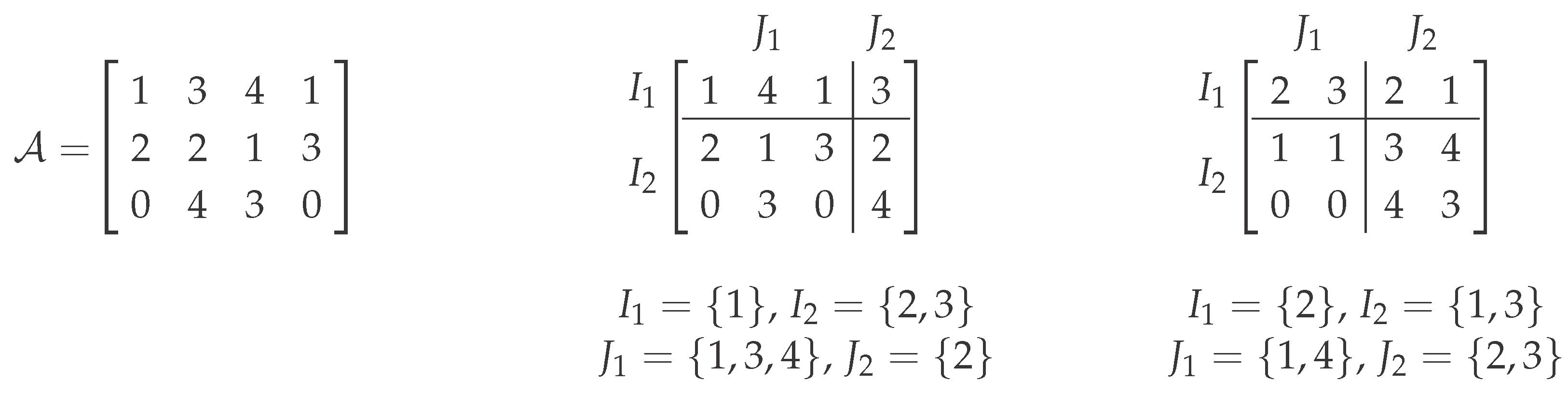
The example shows two (2, 2)-co-clusterings (middle and right) of the same matrix (left-hand side). It demonstrates that by sorting rows and columns according to the co-clustering, the clusters can be illustrated as submatrices of this (permuted) input matrix. The cost of the (2, 2)-co-clustering in the middle is three (because of the two left clusters), and that of the (2, 2)-co-clustering on the right-hand side is one.
Figure 1.
The example shows two (2, 2)-co-clusterings (middle and right) of the same matrix (left-hand side). It demonstrates that by sorting rows and columns according to the co-clustering, the clusters can be illustrated as submatrices of this (permuted) input matrix. The cost of the (2, 2)-co-clustering in the middle is three (because of the two left clusters), and that of the (2, 2)-co-clustering on the right-hand side is one.

Figure 2.
An illustration of the reduction from 3-Coloring. Left: An undirected graph with a proper 3-coloring of the vertices, such that no two neighboring vertices have the same color. Right: The corresponding matrix where the columns are labeled by vertices and the rows by edges with a (3, 3)-co-clustering of cost one. The coloring of the vertices determines the column partition into three columns blocks, whereas the row blocks are generated by the following simple scheme: edges where the vertex with a smaller index is red/blue (dark)/yellow (light) are in the first/second/third row block (e.g., the red-yellow edge {2, 5} is in the first block; the blue-red edge {1, 6} is in the second block; and the yellow-blue edge {3, 4} is in the third block).
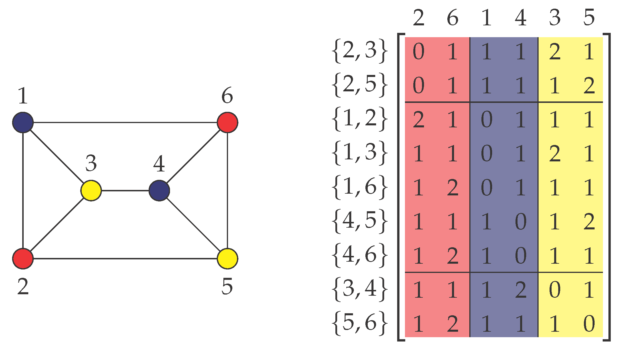
Figure 3.
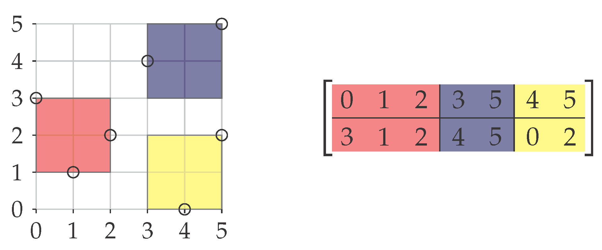
Example of a Box Cover instance with seven points (left) and the corresponding Co-Clustering∞ matrix containing the coordinates of the points as columns (right). Indicated is a (2, 3)-co-clustering of cost two where the column blocks are colored according to the three squares (of side length two) that cover all points.
Figure 3.
Example of a Box Cover instance with seven points (left) and the corresponding Co-Clustering∞ matrix containing the coordinates of the points as columns (right). Indicated is a (2, 3)-co-clustering of cost two where the column blocks are colored according to the three squares (of side length two) that cover all points.

Figure 4.
Example instance of Optimal Discretization (left) and the corresponding instance of Consecutive Co-Clustering∞ (right). The point set consists of white (circles) and black (diamonds) points. A solution for the corresponding Consecutive Co-Clustering∞ instance (shaded clusters) naturally translates into a consistent set of lines.

Table 1.
Overview of results for -Co-Clustering∞ with respect to various parameter constellations (m: number of rows; : alphabet size; : size of row/column partition; c: cost). A ⊛ indicates that the corresponding value is considered as a parameter, where FPT (fixed-parameter tractable (FPT)) means that there is an algorithm solving the problem where the super-polynomial part in the running time is a function depending solely on the parameter. Multiple ⊛’s indicate a combined parameterization. Other non-constant values may be unbounded.
| m | |Σ| | k | ℓ | c | Complexity |
|---|---|---|---|---|---|
| - | - | - | - | 0 | P [Observation 1] |
| - | 2 | - | - | - | P [Observation 1] |
| - | - | 1 | - | - | P [Theorem 4] |
| - | - | 2 | 2 | - | P [Theorem 5] |
| - | 3 | 2 | - | - | P [Theorem 6] |
| - | - | 2 | ⊛ | 1 | FPT [Corollary 2] |
| - | ⊛ | 2 | - | 1 | FPT [Corollary 2] |
| ⊛ | - | ⊛ | ⊛ | ⊛ | FPT [Lemma 2] |
| - | 3 | 3 | 3 | 1 | NP-hard [Theorem 1] |
| 2 | - | 2 | - | 2 | NP-hard [Theorem 2] |
© 2016 by the authors; licensee MDPI, Basel, Switzerland. This article is an open access article distributed under the terms and conditions of the Creative Commons by Attribution (CC-BY) license (http://creativecommons.org/licenses/by/4.0/).
Share and Cite
MDPI and ACS Style
Bulteau, L.; Froese, V.; Hartung, S.; Niedermeier, R. Co-Clustering under the Maximum Norm. Algorithms 2016, 9, 17. https://doi.org/10.3390/a9010017
AMA Style
Bulteau L, Froese V, Hartung S, Niedermeier R. Co-Clustering under the Maximum Norm. Algorithms. 2016; 9(1):17. https://doi.org/10.3390/a9010017
Chicago/Turabian StyleBulteau, Laurent, Vincent Froese, Sepp Hartung, and Rolf Niedermeier. 2016. "Co-Clustering under the Maximum Norm" Algorithms 9, no. 1: 17. https://doi.org/10.3390/a9010017
Note that from the first issue of 2016, this journal uses article numbers instead of page numbers. See further details here.