Article

Series Arc Fault Detection Algorithm Based on Autoregressive Bispectrum Analysis

1
College of Mechanical Engineering and Automation, Huaqiao University, Xiamen 361021, China
2
School of Mechanical and Automotive Engineering, Fujian University of Technology, Fuzhou 350118, China
*
Author to whom correspondence should be addressed.
Algorithms 2015, 8(4), 929-950; https://doi.org/10.3390/a8040929
Submission received: 3 July 2015 / Revised: 24 September 2015 / Accepted: 28 September 2015 / Published: 16 October 2015

Abstract

:
Arc fault is one of the most critical reasons for electrical fires. Due to the diversity, randomness and concealment of arc faults in low-voltage circuits, it is difficult for general methods to protect all loads from series arc faults. From the analysis of many series arc faults, a large number of high frequency signals generated in circuits are found. These signals are easily affected by Gaussian noise which is difficult to be eliminated as a result of frequency aliasing. Thus, a novel detection algorithm is developed to accurately detect series arc faults in this paper. Initially, an autoregressive model of the mixed high frequency signals is modelled. Then, autoregressive bispectrum analysis is introduced to analyze common series arc fault features. The phase information of arc fault signal is preserved using this method. The influence of Gaussian noise is restrained effectively. Afterwards, several features including characteristic frequency, fluctuation of phase angles, diffused distribution and incremental numbers of bispectrum peaks are extracted for recognizing arc faults. Finally, least squares support vector machine is used to accurately identify series arc faults from the load states based on these frequency features of bispectrum. The validity of the algorithm is experimentally verified obtaining arc fault detection rate above 97%.

1. Introduction

Statistical data from fire services show that over 90% of electrical fires are caused by arc faults, over currents, short circuits and leakages [1,2,3,4]. Leakage protectors and over current breakers are respectively used to protect electrical circuits from leakages and over currents presently, but they cannot be used to protect circuits from arc faults. There are three types of arc faults: ground arc fault, parallel arc fault and series arc fault. Parallel and ground arc faults respectively share similar features to ground fault and over current and are thus easy to be detected [5]. However, fault features from series arc faults are usually submerged by load currents and background noise, thus making accurate recognition difficult.
To accurately describe an arc fault in mathematics, some arc fault models were proposed. Gammon and Matthews developed an instantaneous arc model for a resistive-inductive system [6]. This model could predict arc fault currents because arc voltage was a current-dependent function. Another similar arc fault model for alternating current (AC) systems was derived by the probability method [7]. Parise provided a simplified model which could be used to analyze and determine basic parameters such as arc resistance and ignition voltage [8]. To fit with the arc fault scenarios described in UL1699 which was a standard for arc fault circuit interrupter (AFCI), a meta-model based on Mayr and Ayrton models was built [9]. Arc fault models usually provide theoretical bases for arc fault detection.
When arc faults occur in circuits, some abnormal behaviors are found on arc light, arc sounds, arc radiation signals, arc voltages and arc currents. Arc light and arc sounds usually change obviously and they can be used for arc fault detection [10,11]. The study in [12] estimated the amplitude of arc voltage by least error squares method. The voltage was compared with a given threshold value to identify arc faults. Another similar approach for arc fault detection by the amplitude comparison of arc voltage was proposed in [13]. The simulation of the approach was successfully done using a square wave arc model. Charles obtained the radiated electromagnetic energy from arc source using a stick and a loop antenna [14]. He then concluded that the radiation signals could be used for arc fault detection. Although arc fault behaviors of arc light, arc sounds, arc radiation signals and arc voltages are obvious, they appear on stationary sites. Hence, there are some limitations in arc fault detection methods based on these behaviors since the sites, time and intensities of series arc faults are random.
The study in [15] briefly summarized the frequency features of currents. Researchers in the study believed that the high frequency components (greater than 20 kHz) existed in arc fault currents. In the frequency domain, the spectrum energy variations of line currents can be used to detect series arc faults [16]. In many studies, a large quantity of load currents in arc faults and normal states were first acquired. Arc fault features were then found by advanced signal processing approaches, and arc faults were finally discriminated from the load states based on these features. Those advanced approaches are: using the absolute sum value of coefficients in multiresolution signal decomposition [17], combining discrete wavelet transform and wavelet networks [18], using discrete wavelet transform and an artificial neural network [19,20], using Gabor Transform and artificial neural network [21], reconstructing the information entropy of signals in different frequency bands [22], etc.
For this paper, in order to improve the accuracy of arc fault detection, a large number of arc fault high frequency signals will be collected by a transducer to find any common features among arc faults. High frequency signals are usually mixed with Gaussian noise, such as circuit noise and quantization noise from the acquisition process [23]. In order to improve the signal-to-noise ratio (SNR) and the accuracy of arc fault detection, the higher-order spectrum will be introduced in this paper. Higher-order spectrum analysis is emerging as a new useful technique in signal processing; it can describe nonlinear coupling, restrain Gaussian noise and preserve phase information among different frequency components of a random process. The study in [24] introduced the higher-order spectrum in detail. In the third-order case of a random process, the higher-order spectrum reduces to the bispectrum. The two main methods used to estimate the bispectrum are the conventional and the parametric methods [24,25,26,27,28,29]. Raghuvee and Nikias presented two parametric approaches consisting of the third-order recursion method and the constrained third-order mean method to estimate the bispectrum [30,31]. Bispectrum has been widely used in many fields, such as electrical and mechanical equipment condition monitoring and diagnostics [32,33,34], astronomy [35], communication [36,37] and biomedical engineering [38,39].
Bispectrum will be used to extract common features for identifying series arc faults. In order to further improve the identification rate of arc fault, a good classification algorithm is needed. Compared with traditional classification algorithms, such as a neural network algorithm, support vector machine (SVM) can better solve the difficult problems: dimension disaster, over learning, local minima [40,41], etc. It has several merits including convergence to global optimum, good generalization ability and adaptation for some small samples and high dimension data [42,43]. In this research, least squares support vector machine (LSSVM) will be introduced to identify series arc faults.
As mentioned above, many previous studies on arc fault detection have discussed mathematical models, abnormal behaviors in time domain, frequency spectrum, power spectrum, etc., but none of these studies offer autoregressive (AR) model and AR bispectrum analysis for arc fault detection. For the first time, this research will apply AR bispectrum to study arc faults in low-voltage AC circuits.
The remainder of this paper is organized as follows. Section 2 constructs an arc fault experimental platform and collects a large amount of experimental data. Section 3 analyzes different types of load signals in arc faults and normal states based on two main methods: conventional time-frequency domain and AR bispectrum analysis. The conventional time-frequency analysis includes time domain and power spectrum analysis. In bispectrum analysis, an AR model is first modelled, then AR bispectrum is introduced. Common series arc fault features are extracted as input vectors to recognize arc faults. Section 4 introduces LSSVM and applies it to the identification of series arc faults from the load states. Finally, Section 5 summarizes the conclusions of this study.

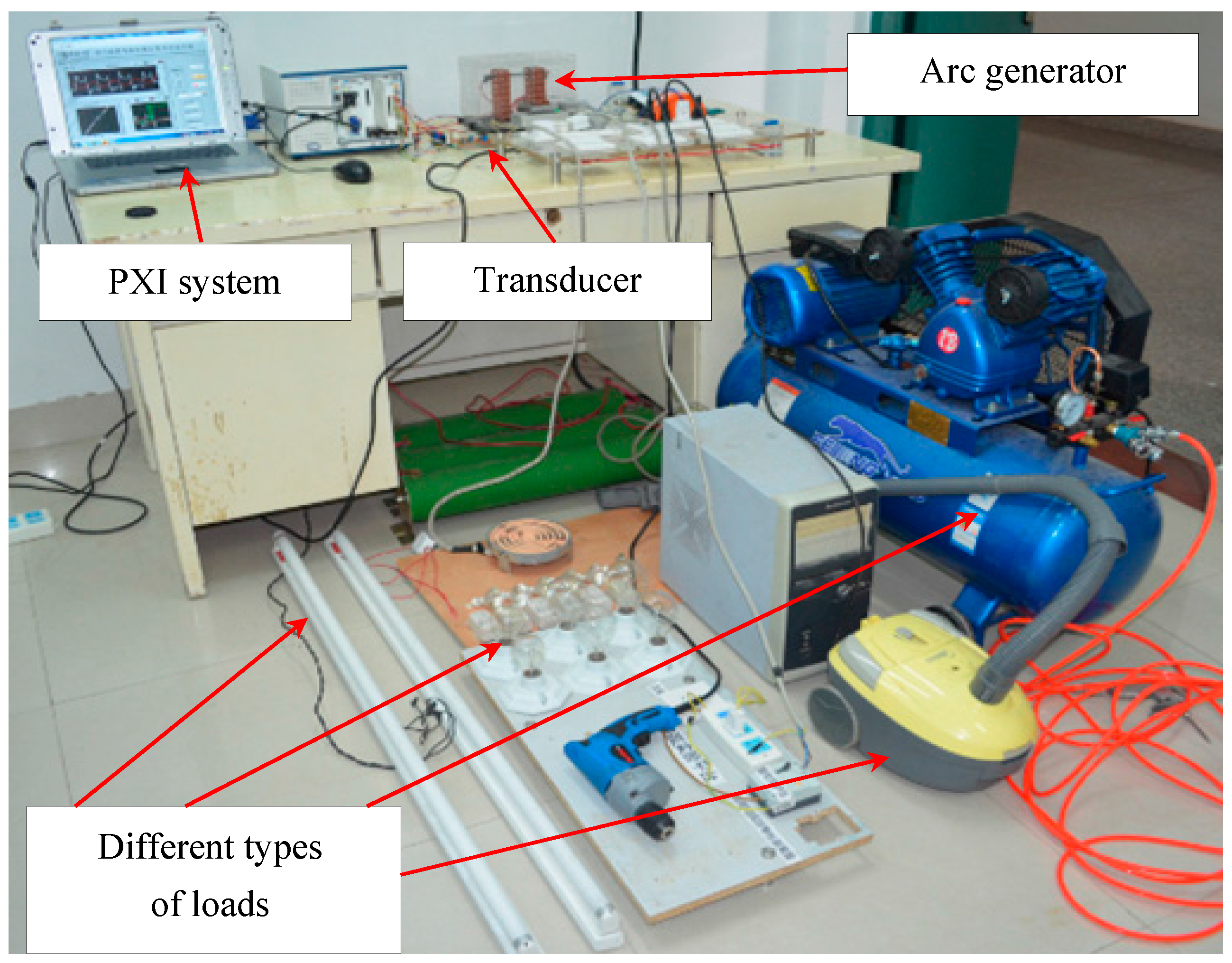
2. Experimental Platform

An arc fault experimental platform which is based on the low-voltage electric standards is constructed as shown in Figure 1. Electrical standards include UL1699, IEC 62606: 2013 and GB/T 31143-2014 which are used as reference standards to construct the experimental platform. Typical experimental loads are composed of six 50 W halogen lamps, a 0.75 kW electrical hand drill, two 40 W fluorescent lamps, a 0.35 kW computer, a 1.2 kW electric stove, a 1 kW dimming lamp, a 1.2 kW vacuum cleaner, a 1.1 kW air conditioning unit and a 2.2 kW air compressor. The arc generator used for simulations of arc faults in circuits consists of a stationary electrode and a moving electrode. A PXI (the abbreviated form of the peripheral component interconnection extension for instrumentation) data acquisition system and a high frequency transducer are used to acquire a large number of high frequency signals in circuits. The band width of PXI system is 100 MHz. Different types of load signals in arc faults and normal states are acquired through this experimental platform, and they will be used to analyze the common features of arc faults in the following section.
Figure 1. Experimental platform of arc faults.
Algorithms 08 00929 g001

3. Signal Analysis

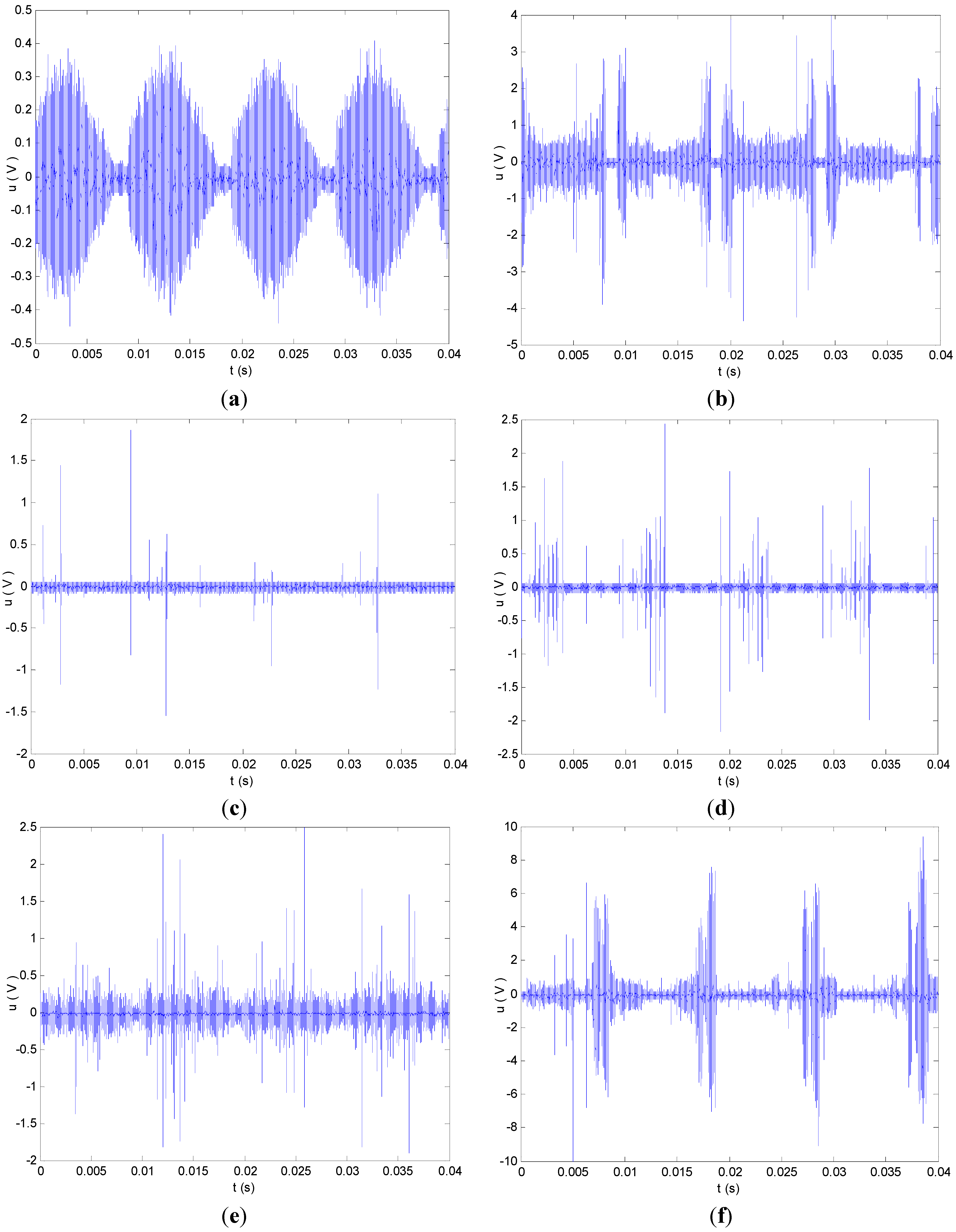
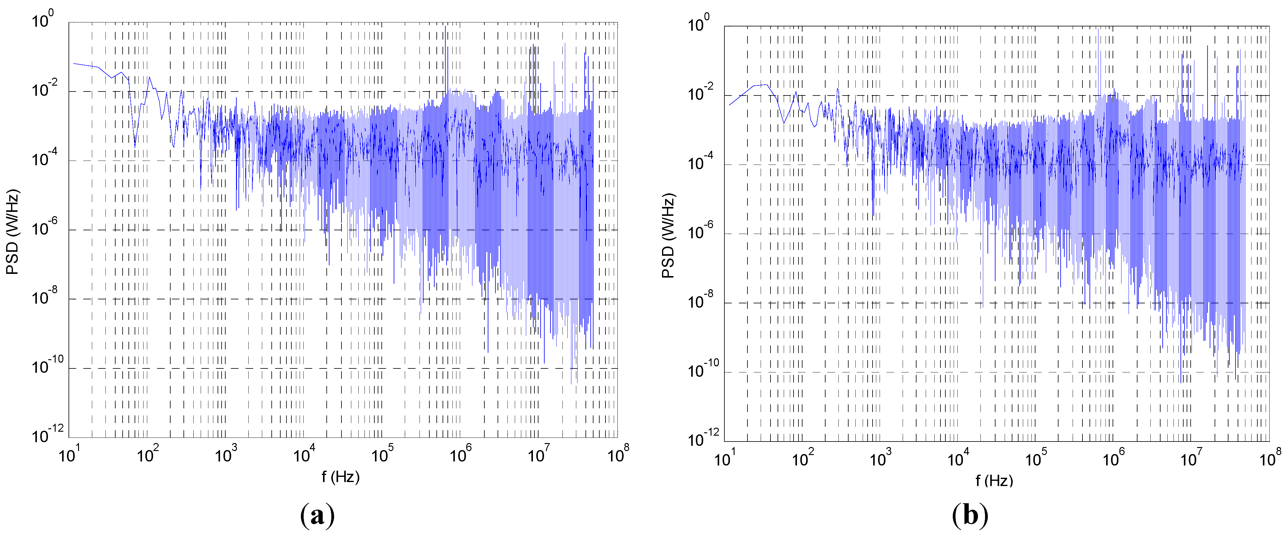
3.1. Conventional Time-Frequency Analysis

High frequency signals were discovered during numerous arc fault experiments. They could reflect the dynamic arc discharge process and be acquired using high frequency transducers [14]. At first, air molecules in the wire gap are ionized in the initiation of arc discharge, and the motion of plasma is then intensified further. According to electromagnetic theory, great quantities of high frequency signals are initially released. The signals are then gradually reduced during the remainder of the current cycle [14]. As a result, high frequency signals are produced periodically when arc faults exist in circuits. However, these signals are uncertain as a result of the unknown external conditions including the effects of electrode materials, surface states, oxide layers, adsorbed gases, arc currents, arc gaps of dielectric materials, etc.
Figure 2. Detected high frequency signals of different load states. (a) Halogen lamp normal; (b) Halogen lamp arc fault; (c) Vacuum cleaner normal; (d) Vacuum cleaner arc fault; (e) Electrical drill normal; (f) Electrical drill arc fault.
Algorithms 08 00929 g002
In order to find the features of arc faults, some typical load signals are selected for analysis. The high frequency signals of different loads in arc faults and normal states are shown in Figure 2. There are many high frequency signals and short pulses generated during the arcing process when the loads work in arc fault states as shown in Figure 2b,d and f. The high frequency signals with big amplitudes are densely distributed. However, high frequency signals can be also acquired during the normal states as shown in Figure 2a,c and e.
As a result of the switch transformers alternating between on/off state, there are many high frequency signals generated in current cycles when the halogen lamps work in the normal state as shown in Figure 2a. Similarly, when the vacuum cleaner and the electrical drill work in normal states, some random interference pulses appear in the circuits as shown in Figure 2c,e. Due to electric brush motors in the vacuum cleaner and electrical drill, electrical discharge occurs and produces many high frequency signals when the electric brush changes the current phase. Electric sparks can be seen from the electrical drill windows even when working in the normal states. The electric sparks are caused by load arcs which are not dangerous but are similar to fault arcs. It is usually very difficult to discriminate load arcs directly from measured frequency signals.
The analysis above indicates that it is difficult to find a reasonable numerical threshold to classify arc faults and the normal states in all loads by simply inspecting the constant amplitude of the high frequency signals. This is because that arc fault signals are usually mixed with much interference consisting of circuit noise, quantization noise from the acquisition process, random noise from electric parts, etc. They are both close to the Gaussian distribution. As a result of their existence, the SNR decreases considerably. The frequency aliasing is hard to overcome.
In frequency domain, the power spectra of vacuum cleaner are shown in Figure 3. The frequency distributions of arc faults and normal states in power spectra are similar. As we know, the power spectrum is based on second-order statistics. Signals are only analyzed by the amplitude (e.g. Figure 2c,e and Figure 3a,b) but lack phase coupling information. So the power spectrum may fail in providing a satisfactory description in a non-Gaussian or nonlinear process. In addition, there are many high frequency signals generated in current cycles when the vacuum cleaner works in normal state. The power spectrum applies the Fourier transform to all signals and is sensitive to the Gaussian noise. Hence it is difficult to distinguish the effective components from the mixed signals of arc faults through the power spectrum. That is to say, it is difficult to identify series arc faults from the load states. Generally speaking, arc fault high frequency signals are random, nonlinear and non-Gaussian. Since bispectrum is a powerful technique in processing random signals, it will be introduced to analyze arc fault signals in the following section.
Figure 3. The power spectra of vacuum cleaner. (a) Normal; (b) Arc fault.
Algorithms 08 00929 g003

3.2. Bispectrum Analysis

Higher-order spectrum and higher-order cumulants are useful tools in describing the dynamic features and processing signals [44]. Bispectrum is the two-dimensional Fourier transform of third-order cumulants and is the simplest higher-order spectrum. It is widely used in describing the nonlinear coupling, restraining Gaussian noise and preserving the phase information of random signals. At present, there are many methods to estimate the bispectrum. A parametric method based on the AR model is introduced to study arc faults in this section.

3.2.1. AR Model and Third-Order Cumulants

According to the analysis results in Section 3.1, arc fault is an obvious random process. So it is very difficult for us to build a mathematical function to describe the variation rules with time. However, we may introduce time series analysis theory to reveal the correlation among the acquired data from arc faults. Here, the AR model is introduced. As a result of environmental impacts, circuit noise, quantization noise and load disturbances, there is much interference mixed in arc fault signals. The random signals which exist in arc faults are assumed to be interfered by the non-Gaussian white noise a(t) whose mean value is zero. The zero-mean non-Gaussian colored noise u(t) containing abundant useful dynamic information of arc faults is assumed to be the output of AR process driven by a(t) [30,44]. Therefore, the time series AR model of arc fault can be described as
u ( t ) = k = 1 q φ k u ( t k ) = a ( t ) , ( t = 1 , 2 , 3 , )
where q is the order of model AR(q), φ k ( k = 1 , 2 , , q ) is the autoregressive coefficient and a(t) is the input signal.
According to the relationship between cumulants and moments in statistical theory, the third-order cumulants of u(t) can be expressed as
C 3 u ( τ 1 , τ 2 ) = E [ u ( t ) u ( t + τ 1 ) u ( t + τ 2 ) ] E [ u ( t ) ] E [ u ( t + τ 1 ) u ( t + τ 2 ) ] E [ u ( t + τ 1 ) ] E [ u ( t + τ 2 ) u ( t ) ] E [ u ( t + τ 2 ) ] E [ u ( t ) u ( t + τ 1 ) ] + 2 E [ u ( t ) ] E [ u ( t + τ 1 ) ] E [ u ( t + τ 2 ) ]
where τ 1 and τ 2 are lags. The mean of u(t) can be denoted as μ u = E [ u ( t ) ] and the correlation function can be expressed as ρ u ( τ ) = E [ u ( t ) u ( t + τ ) ] . Then Equation (2) can be denoted as
C 3 u ( τ 1 , τ 2 ) = E [ u ( t ) u ( t + τ 1 ) u ( t + τ 2 ) ] μ u ρ u ( τ 2 τ 1 ) μ u ρ u ( τ 2 ) μ u ρ u ( τ 1 ) + 2 μ u 3
After the preprocessing, the mean value of u(t) is zero, namely, μ u = 0 . Therefore, Equation (3) can be simplified as
C 3 u ( τ 1 , τ 2 ) = E [ u ( t ) u ( t + τ 1 ) u ( t + τ 2 ) ]
Here the third-order cumulants of u(t) equal to its third-order moments. For the input signal a(t), it has the following properties:
{ E [ a ( t ) a ( t + τ 1 ) ] = σ a 2 δ ( τ 1 ) E [ a ( t ) a ( t + τ 1 ) a ( t + τ 2 ) ] = γ δ ( τ 1 , τ 2 ) E [ a ( t ) u ( t τ 1 ) ] = 0   ( τ 1 0 , τ 2 0 )
where σ a 2 is the variance of a(t), δ ( τ 1 ) is the one-dimensional unit impulse function, δ ( τ 1 , τ 2 ) is the two-dimensional unit impulse function and the coefficient γ = E [ a 3 ( t ) ] 0 .
For a stationary physical process, Equation (1) can be expressed by using third-order cumulants of u(t) [30,31]:
C 3 u ( - τ 1 , - τ 2 ) + k = 1 q φ k C 3 u ( k - τ 1 , k - τ 2 ) = γ δ ( τ 1 , τ 2 )
When τ 1 = τ 2 = 0 1 , 2 , , q , Equation (6) can be transformed in matrix:
C Φ = Γ
where C = [ C 3 u ( 0 , 0 ) C 3 u ( 1 , 1 ) C 3 u ( q , q ) C 3 u ( 1 , 1 ) C 3 u ( 0 , 0 ) C 3 u ( q 1 , q 1 ) C 3 u ( q , q ) C 3 u ( 1 q , 1 q ) C 3 u ( 0 , 0 ) ] , Φ = [ 1 φ 1 φ q ] , Γ = [ γ 0 0 ] . C is a Toeplitz matrix but in general is not symmetric, φ k ( k = 1 , 2 , , q ) is the AR model parameter to be estimated.
Now, when solving Equation (7), a crucial action should be taken: determine the order of AR model. This problem can be solved by the cumulant matrix C e with the singular value decomposition technique [45]. Here C e is the third-order cumulant matrix of u(t). It can be decomposed as
C e = U Σ V H
where U and V are unitary matrices, Σ is an matrix whose elements are zero except possibly along its main diagonal and V H is the complex conjugate transpose of V. The diagonal elements of Σ are ordered as
λ 1 λ 2 λ n 0
The diagonal element λ n is called as the singular value of C e . The normalized ratio of Frobenious norm can be expressed as
R ( q ) = [ λ 1 2 + λ 2 2 + + λ q 2 ] 1 2 [ λ 1 2 + λ 2 2 + + λ n 2 ] 1 2 , q = 1 , 2 , , n
The number q can be regarded as the order of the AR model when R(q) ≥ 0.995.
At last, Equation (7) can be solved by the least squares method to obtain the AR model parameter φ k ( k = 1 , 2 , , q ) . Here the AR model of the mixed high frequency signals can be used to quantitatively describe the nonlinear coupling relationships of arc fault signals. The next task is to extract series arc fault features through bispectrum based on the AR model.

3.2.2. AR Bispectrum

AR Bispectrum is a type of bispectrum which is estimated through an AR model parametric method. It will be briefly introduced in this section.
In Equation (1), if the system impulse response is h(t), the output u(t) can be described as
u ( t ) = β = h ( β ) a ( t β )
Substituting Equation (11) into Equation (4), then we have
C 3 u ( τ 1 , τ 2 ) = E [ β = h ( β ) a ( t β ) × χ = h ( χ ) a ( t + τ 1 χ ) × ε = h ( ε ) a ( t + τ 2 ε ) ] = β = χ = ε = h ( β ) h ( χ ) h ( ε ) × E [ a ( t β ) a ( t + τ 1 χ ) a ( t + τ 2 ε ) ]
As a result of δ ( i , j ) = { 1 , i = j = 0 0 , others , γ = E [ a 3 ( t ) ] 0 , Equation (12) can be simplified as
C 3 u ( τ 1 , τ 2 ) = β = χ = ε = h ( β ) h ( χ ) h ( ε ) γ δ ( τ 1 χ + β , τ 2 ε + β ) = γ β = h ( β ) χ = h ( χ ) δ ( τ 1 χ + β ) ε = h ( ε ) δ ( τ 2 ε + β ) = γ β = h ( β ) h ( τ 1 + β ) h ( τ 2 + β )
According to the definition of higher-order spectrum, third-order cumulants spectrum (usually called bispectrum) is defined as the two-dimensional Fourier transform of third-order cumulants:
S 3 u ( ω 1 , ω 2 ) = τ 1 = τ 2 = C 3 u ( τ 1 , τ 2 ) e j ( ω 1 τ 1 + ω 2 τ 2 )
Here the imaginary number j = 1 . Substituting Equation (13) into Equation (14), then we have
S 3 u ( ω 1 , ω 2 ) = λ H ( ω 1 ) H ( ω 2 ) H * ( ω 1 + ω 2 )
where the frequency transfer function H ( ω ) β = h ( β ) e j ω β and H * ( ω 1 + ω 2 ) is the complex conjugate of H ( ω 1 + ω 2 ) [31,46].The frequency transfer function of the q-th order AR process in Equation (1) can be further expressed as
H ( ω ) = 1 1 + k = 1 q φ k e j ω k
To reduce the computational complexity of the bispectrum, bispectrum slice will be introduced. The one-dimensional slices of the bispectrum are the reconstructed spectra. For ω = ω1 = ω2 and according to Equation (15), the calculation of 1½-dimensional slices of the bispectrum is given by
S 3 u ( ω , ω ) = λ H 2 ( ω ) H * ( 2 ω )
The 1½-dimensional slices usually achieve high resolution ability and have quick calculation speed [47]. They can also reflect the nonlinearity, the quadratic phase coupling information and restrain Gaussian noise of a random process. They can be used to analyze arc fault features quickly.

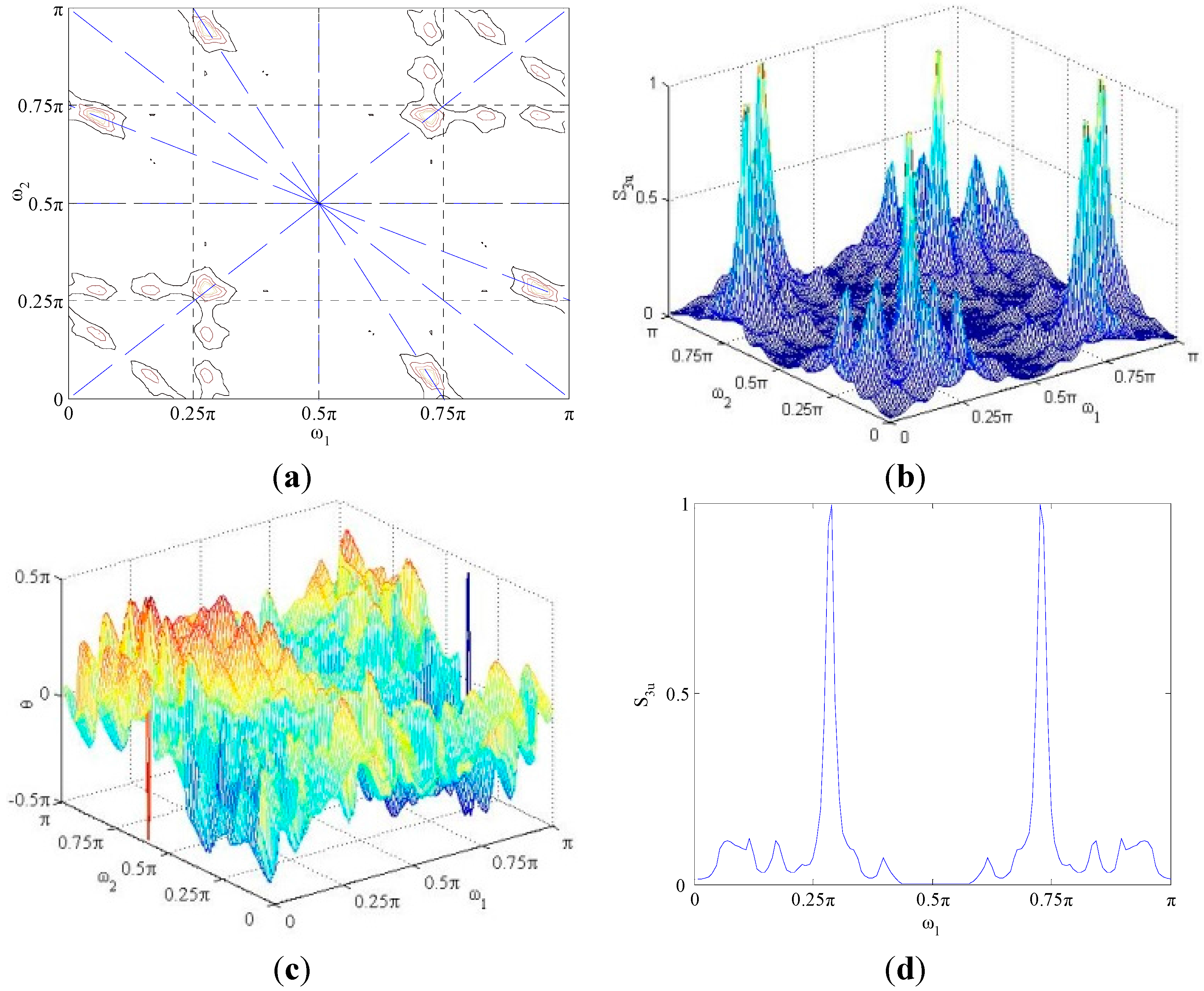
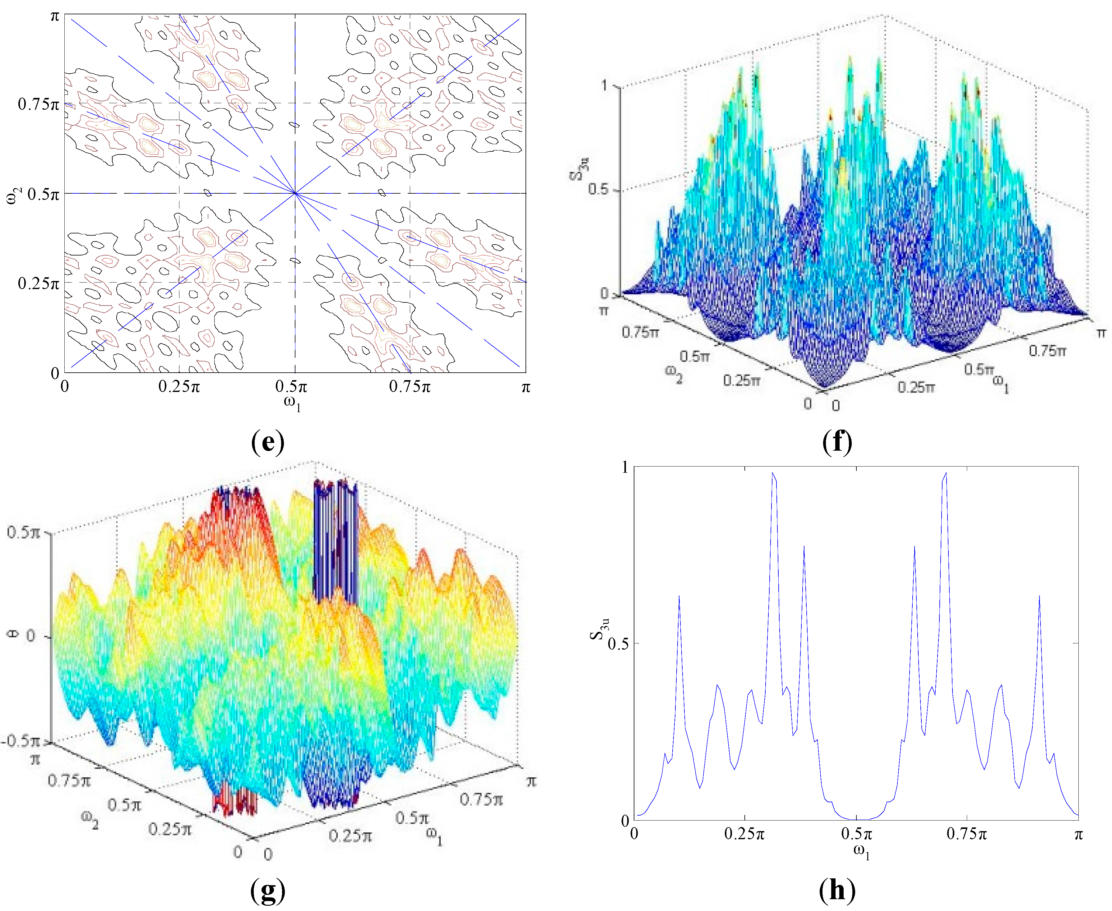
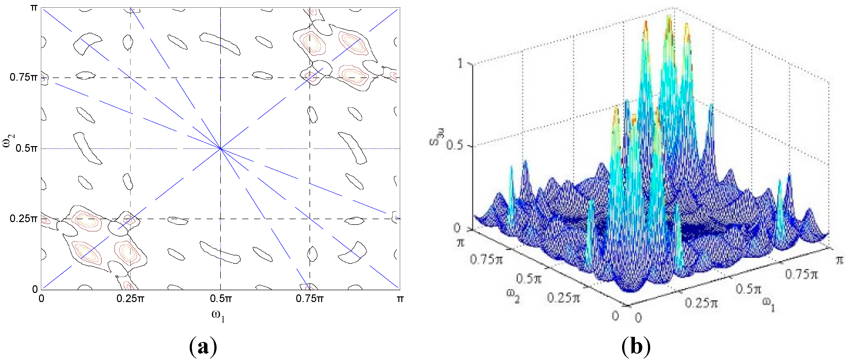
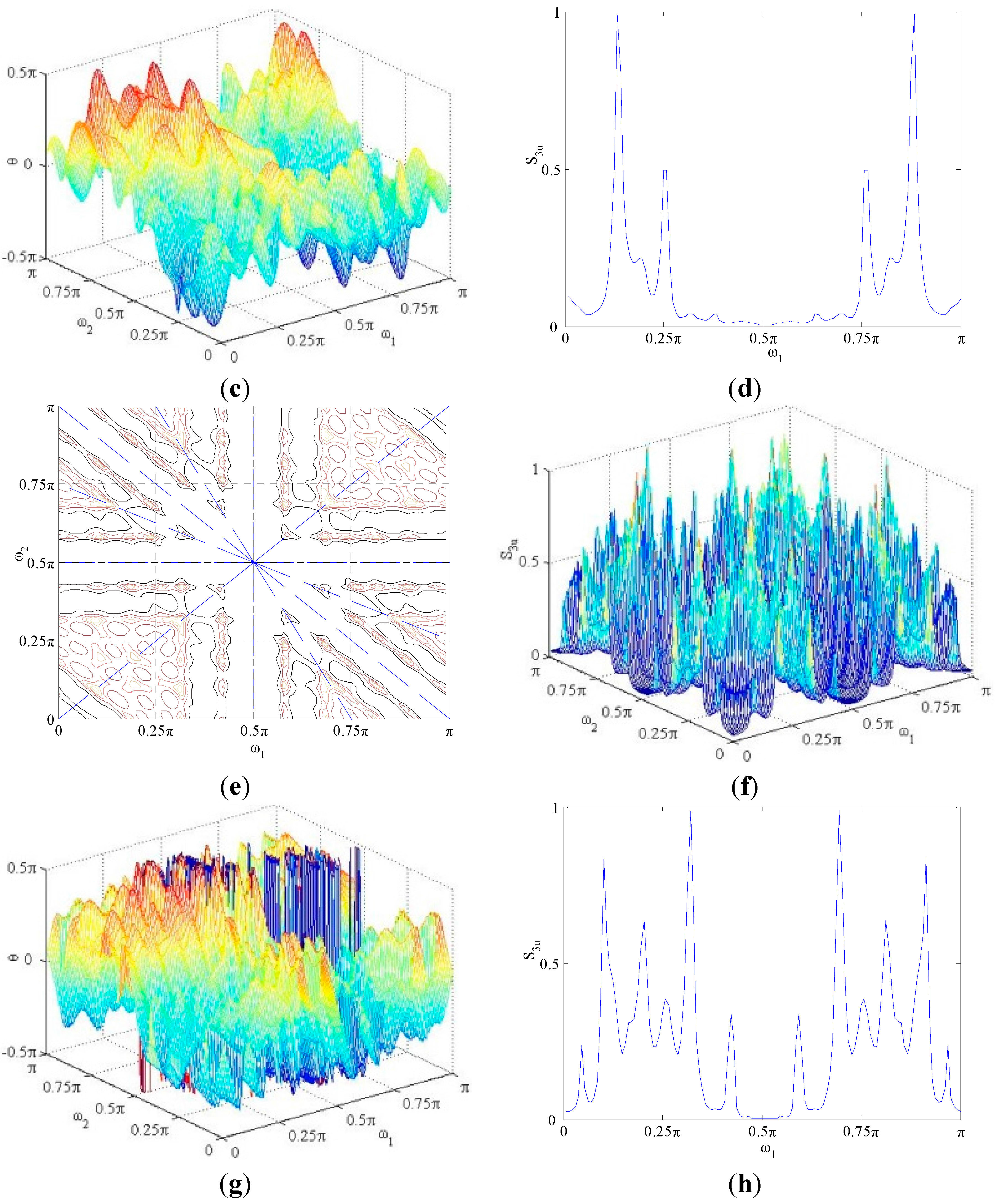
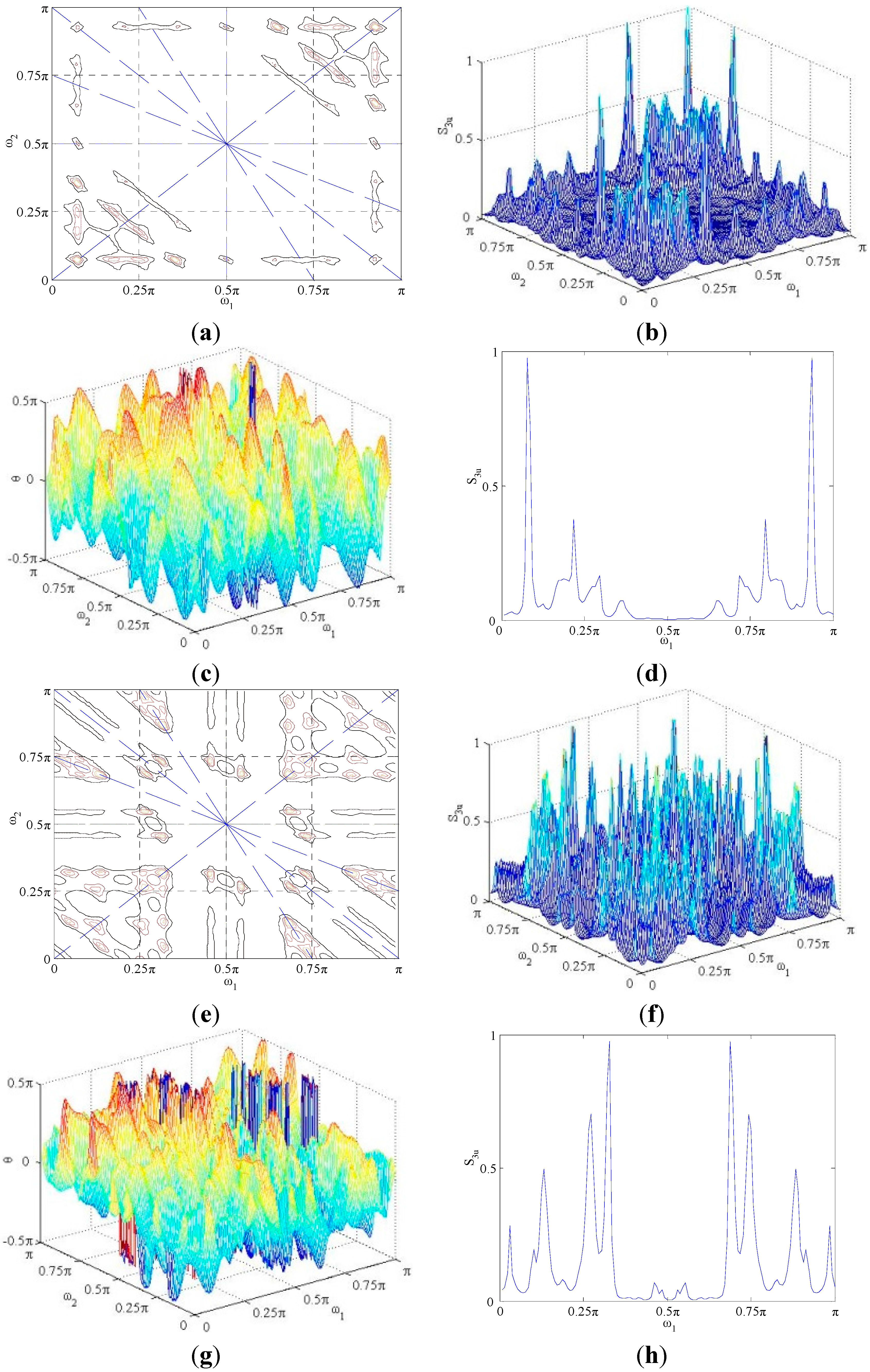
3.2.3. Bispectrum Features of Arc Faults

The contours, amplitudes, phase angles and the 1½-dimensional slices of different load bispectra are plotted as shown in Figure 4, Figure 5 and Figure 6. According to the differences between the normal state and arc fault bispectra, it is demonstrated that more information about the nonlinear dynamic features of the load signals is given by the bispectra. When series arc faults occur in circuits, the energy distribution which can be discovered from the contours becomes diffused.
Since the power spectrum is phase blind, it is unable to detect the presence of phase coupling. However, the bispectrum gives an indication of the correlation between the phases of different frequency components ω 1 and ω 2 . In addition, the power spectrum also applies the Fourier transform to all signals and is sensitive to Gaussian noise. In contrast, the bispectrum can eliminate the additive Gaussian noise and provide information of the phase coupling. The phases of electrical load arc faults are different from those of normal states, where the former increase suddenly and randomly in some frequency domain while the latter change smoothly in most frequency domain. Since the capacitive and the inductive reactance of fault arc are unstable, they may change randomly.
As shown in the analysis of arc fault contours (Figure 4, Figure 5 and Figure 6) and the symmetry features of the bispectrum, all the valuable information in the arc fault signal is contained in the bispectra in the inner triangular domain ω 2 0 , ω 1 ω 2 and ω 1 + ω 2 π . Therefore, the spectrum is sufficient for the description of all bispectrum features and the symmetry features are given by:
S 3 u ( ω 1 , ω 2 ) = S 3 u ( ω 2 , ω 1 ) = S 3 u * ( ω 1 , ω 2 ) = S 3 u * ( ω 2 , ω 1 ) = S 3 u ( ω 1 , ω 1 ω 2 ) = S 3 u ( ω 1 ω 2 , ω 1 ) = S 3 u ( ω 2 , ω 1 ω 2 ) = S 3 u ( ω 1 ω 2 , ω 2 )
In the inner triangular domain, the highest peaks can be found in each plot. The peaks of the bispectra indicate the process is non-Gaussian and the nonlinear coupling does exist in the arc fault signals. One possible reason is the randomness of the fault arc resistance. The information of the peaks is similar, and proves they are effective in reflecting the information of the dominant frequency components of the non-Gaussian nonlinear arc fault signals.
When the loads work in normal, the background noise and working processes are treated as stationary random processes, and there are few peaks in the bispectrum graphs. When series arc faults occur in circuits, as a result of the coupling relations of different high frequency components generated by arc faults, bispectrum peaks gradually change from concentrated distribution to dispersed and become mixed and disordered. The number of bispectrum peaks is evidently increased. There are increased numbers of high peaks in the arc fault bispectrum as a result of strong correlation in some frequency. The arc fault becomes more serious and the nonlinearity becomes stronger.
The above dynamic features of load states are also performed in the slices of bispectra. Furthermore, the 1½-dimensional slices of bispectra are easier to calculate than bispectra. The phase coupling frequency components can also be extracted from the Gaussian noise environment. Bispectrum peak numbers of arc faults increase obviously, and the highest bispectrum peak positions of arc faults move towards ω 1 = 0.5 π . Therefore, the attended phase coupling components and their generated components in the 1½-dimensional slices of bispectra can be used for arc fault detection. However, it is hard to find constant thresholds to classify normal states and arc faults in all loads. Thus, a good classification algorithm is needed.
Figure 4. AR bispectra of halogen lamp. (a) Normal contour; (b) Normal amplitude; (c) Normal phase angle; (d) Normal 1½-D slices; (e) Arc fault contour; (f) Arc fault amplitude; (g) Arc fault phase angle; (h) Arc fault 1½-D slices.
Algorithms 08 00929 g004aAlgorithms 08 00929 g004b
Figure 5. AR bispectra of vacuum cleaner. (a) Normal contour; (b) Normal amplitude; (c) Normal phase angle; (d) Normal 1½-D slices; (e) Arc fault contour; (f) Arc fault amplitude; (g) Arc fault phase angle; (h) Arc fault 1½-D slices.
Algorithms 08 00929 g005aAlgorithms 08 00929 g005b
Figure 6. AR bispectra of electrical drill. (a) Normal contour; (b) Normal amplitude; (c) Normal phase angle; (d) Normal 1½-D slices; (e) Arc fault contour; (f) Arc fault amplitude; (g) Arc fault phase angle; (h) Arc fault 1½-D slices.
Algorithms 08 00929 g006
Compared with traditional classification algorithms, such as a neural network algorithm, SVM can better solve the difficult problems listed as follows: dimension disaster, over learning, local minima [40,41], etc. It has several merits consisting of convergence to global optimum, good generalization ability and adaptation for some small samples and high dimension data [42,43]. To better discriminate arc fault states from load states, the frequencies ω 1 and ω 2 are selected as the input vector. Based on the features including distribution regularities of bispectrum peaks, SVM is introduced to classify series arc faults and the normal states in the following section.

4. Arc Fault Identification

The SVM algorithm which is based on statistical learning theory has been successfully used to solve linear regression, pattern recognition and classification problems [40]. The LSSVM algorithm which has been developed by Suykens and Vandewalle [42] is a new deformation algorithm based on the traditional SVM. It can reduce computing complexity and guarantee the accuracy of data classification simultaneously. The frequencies ω 1 and ω 2 are selected as the input vector x.
The feature vector x is mapped from the original to the high dimensional feature space by nonlinear transformation f(x). Then, the optimal classification plane is found in the high dimensional feature space. According to the structural risk minimization principle, the constrained optimization problem corresponding to the original classification problem can be expressed as follows:
{ min ( 1 2 V T V + C 2 i = 1 m ξ i 2 ) s.t.   y i ( V T f ( x i ) + b ) = 1 ξ i   ( i = 1 , ,   m )
where V is a weight vector, C is the penalty parameter, m is the number of samples, ξ i is the relaxation coefficient and b is a bias term. The output result of classification is y i = { 1 if   x i class  1 1 if   x i class 2 [40,42,48].
In order to solve the constrained optimization problem, Lagrange multipliers α i is introduced. Equation (19) is transformed to the unconstrained objective function as
L ( V , ξ i , α i , b ) = 1 2 V T V + C 2 i = 1 m ξ i 2 i = 1 m α i { y i [ V T f ( x i ) + b ] 1 + ξ i }
According to the Karush-Kuhn-Tucker condition, let the derivative to V, b, α i , ξ i of Equation (20) equal to 0, then the equation can be expressed as
{ y i ( V T f ( x i ) + b ) 1 + ξ i = 0 V = i = 1 m α i y i f ( x i ) i = 1 m α i y i = 0 α i = C ξ i   ( i = 1 , , m )
Furthermore, Equation (21) can be organized into a matrix form
( Ω y y T 0 ) ( α b ) = ( R 0 )
where R =   ( 1 , , 1 ) T , y =   ( y 1 , , y m ) T , α = ( α 1 , , α m ) T , element in the positive definite matrix Ω is Ω i j = y i y j f T ( x i ) f ( x j ) + δ ( i , j ) C = y i y j K ( x i , x j ) + δ ( i , j ) C , δ ( i , j ) = { 1 , i = j = 0 0 , others . On the basis of Mercer condition, K ( x i , x j ) = f T ( x i ) f ( x j ) is defined as a kernel function. According to the features of arc fault signals, the radial basis function (RBF) is selected as the kernel function which is widely used in classification cases.
Hence the optimization problem of Equation (19) can be solved by using Equation (22), where α and b can be solved through least square method [42]. The identification result of the loads states by LSSVM can be described as
y * ( x ) =sgn ( i = 1 m α i y i K ( x , x i ) + b )
The frequencies ω 1 and ω 2 are selected as the input vector x. The main procedures for arc fault identification are listed as follows:
(1)
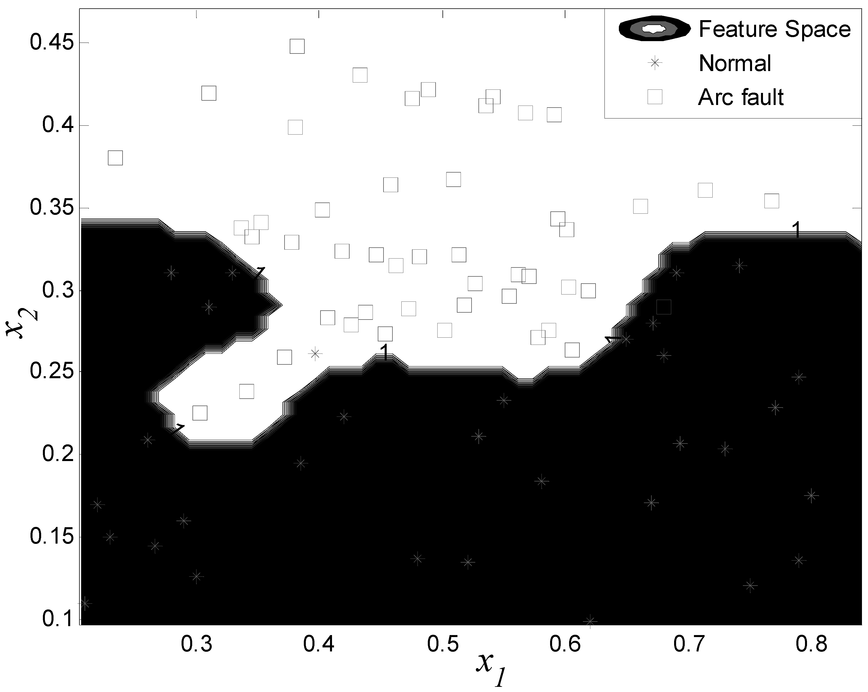
Selection of sample set for LSSVM. The input used the feature vector x including the frequencies x 1 and x 2 . The output was the classification result y. The status of output contained −1 and 1. The “−1” represented the normal state and “1” represented arc fault state.
(2)
Construction of the training set (x, y). From the experimental data of nine types of typical loads in different working states, three hundred and sixty samples were chosen for further processing. Two hundred and eighty samples of those samples were treated as the training samples and the remainder were treated as testing samples. The training set of recognizer was listed in Table 1.
Table 1. The training set of recognizer.
Samples123280
x10.1521π0.3534π0.6171π0.8051π
x20.2213π0.2514π0.3502π0.1586π
y−111−1
(3)
Selection of LSSVM parameters. The RBF can be described as
K ( x i , x j ) = exp ( x i x j 2 / σ 2 )
where σ2 is the kernel parameter. At first, the initial kernel parameter σ2 and the penalty parameter C were selected. Then, the ten-fold cross-validation method was applied to optimize the parameters through the training set. According to the method, the training set was equally divided into ten subsets which were mutually disjoint. The entire method would be repeated ten times. Each time, one of the ten subsets was selected as a new test subset and the other nine subsets were placed together to form a new training subset. The nine subsets were used for training and the tenth subset was used for testing. After repeating ten times, the average error of the ten trials was computed. Finally, the optimal parameters were obtained when the error was the minimum [49].
(4)
Arc fault identification. The testing samples were input into the arc fault recognizer. Then the identification results were compared with the real results. Finally, the generalization ability of recognizer was evaluated based on error rate which could be calculated as
e = i = 1 p | y i * y i | 2 p × 100 %
where p was the number of testing samples and y i * was the classification result.
From the above procedures of arc fault identification, the arc fault recognizer was proposed. The kernel parameter σ2 = 0.54 and the penalty parameter C = 7.1 were obtained by the ten-fold cross-validation method. The identification results are shown in Figure 7 where “*” represents the normal states and “□” represents arc faults of the loads. The testing samples can be identified from the feature vector space. If the testing sample appears on the arc fault feature space in Figure 7, it means an arc fault has occurred in the circuit; otherwise, there is no arc fault. The identification results are the globally optimal solution in that RBF kernel function parameters. The optimal classification plane of arc faults and the normal states can be found in the high dimensional feature space.
Figure 7. Arc fault identification results.
Algorithms 08 00929 g007
After completing sample experiments, the actual results and the classified results are listed in Table 2. The results show the average error rate of LSSVM is 2.6%. Hence, the arc fault identification rate is 97.4%. Since some weak arc fault signals are added to the testing samples, the frequency of the arc fault is very close to that of the normal state. Therefore, the LSSVM recognizer fails to classify the arc faults from the normal states. This limitation can be improved in future works.
Table 2. Confusion matrix for LSSVM recognizer.
Actual ResultsClassified Results
NormalArc Fault
Normal96.875%3.125%
Arc Fault2.083%97.917%

5. Conclusions

AR Bispectrum analysis has been applied in many signal processing cases, but not previously in the analysis of arc faults in low-voltage AC circuits. Therefore, application of said analysis in this research would represent a first. Arc fault features are extracted to realize detection of series arc faults by AR bispectrum. The main conclusions in detail are listed as follows:
(1)
High frequency signals of circuits increase frequently when series arc faults occur in circuits, but they are usually mixed with much interference.
(2)
An AR model of arc fault is established to describe the coupling relationship of the mixed high frequency signals and reflect the dynamic characteristics of arc faults.
(3)
According to the AR bispectrum analysis on nine types of typical experimental loads which are mentioned in electrical standards, the signal phase information of arc fault is kept and the influence of noise such as Gaussian noise is restrained effectively. AR bispectrum analysis is more effective than power spectrum and time-domain analysis. When series arc faults occur, the numbers of spectrum peaks increase obviously; the distribution of spectrum peaks tends to diffuse and the bispectrum slices are also dispersed. To better describe series arc faults, bispectrum frequency features including distribution regularities of bispectrum peaks are extracted as support vectors.
(4)
Based on the above features of bispectrum, LSSVM is successfully used to discriminate arc faults from working states in different loads. The whole algorithm has been well run in the computer and has been verified through the arc fault experimental platform. The arc fault detection rate is over 97%. The result shows that the developed algorithm has good generalization ability in different loads’ arc fault detection. For future research, in terms of algorithm improvement, arc fault detection rate will be further advanced. Furthermore, this algorithm may be applied in direct current (DC) arc fault detection, such as arc faults in photovoltaic systems and automotive power supply systems.

Acknowledgments

This work was supported by the Fujian Science & technology key project (2013H0028), the Xiamen Science & technology project (3502Z20143043) and the Quanzhou Science & technology project of China (2014Z114).

Author Contributions

Kai Yang proposed the detection algorithm and prepared the whole manuscript. Rencheng Zhang supervised the overall research and critical revision of the paper. Shouhong Chen and Fujiang Zhang participated in the algorithm simulation and draft writing. Jianhong Yang participated in the algorithm design. Xingbin Zhang assisted in the experiments.

Conflicts of Interest

The authors declare no conflict of interest.

References

  1. Fire Department of Ministry of Public Security. China Fire Services (2014); Yunnan People’s Publishing House: Kunming, China, 2014; pp. 396–407. (In Chinese) [Google Scholar]
  2. Si, G. Analysis on China’s electrical fire situation and feature from 2008 to 2012. Fire Sci. Technol. 2014, 33, 569–572. [Google Scholar]
  3. Vadoli, C.N. Lessons learned from electrical circuit analysis in support of a fire probabilistic risk assessment. In Proceedings of the International Topical Meeting on Probabilistic Safety Assessment and Analysis, Wilmington, NC, USA, 13–17 March 2011; pp. 711–720.
  4. Lee, D.A.; Trotta, A.M.; King, W.H., Jr. New Technology for preventing residential electrical fires: Arc-fault circuit interrupters (AFCIs). Fire Technol. 2000, 36, 146–162. [Google Scholar] [CrossRef]
  5. Gregory, G.D.; Wong, K.; Dvorak, R. More about arc-fault circuit interrupters. IEEE Trans. Ind. Appl. 2004, 40, 1006–1011. [Google Scholar] [CrossRef]
  6. Gammon, T.; Matthews, J. Arcing-fault models for low-voltage power systems. In Proceedings of the IEEE Industrial and Commercial Power Systems Technical Conference, Clearwater Beach, FL, USA, 7–11 May 2000; pp. 119–126.
  7. Wu, H.R.; Li, X.H.; Stade, D.; Schau, H. Arc fault model for low voltage AC systems. IEEE Trans. Power delivery. 2005, 20, 1204–1205. [Google Scholar] [CrossRef]
  8. Parise, G.; Martirano, L.; Laurini, M. Simplified arc-fault model: The reduction factor of the arc current. IEEE Trans. Ind. Appl. 2013, 49, 1703–1710. [Google Scholar] [CrossRef]
  9. Andrea, J.; Schweitzer, P.; Martel, J.M. Arc fault model of conductance application to the UL1699 tests modeling. In Proceedings of the 2011 IEEE 57th Holm Conference on Electrical Contacts, Minneapolis, MN, USA, 11–14 September 2011; pp. 37–42.
  10. Yang, J.H.; Zhang, R.C.; Du, J.H. Study on application of arcing protective system faults based on multiple information fusion. High Voltage Appar. 2007, 43, 194–196. (In Chinese) [Google Scholar]
  11. Zhang, R.C.; Yang, J.H.; Du, J.H. Study on in-process detection and diagnosis of faults arc based on early sounds signature and intermittent chaos. Key Eng. Mat. 2008, 381, 611–614. [Google Scholar] [CrossRef]
  12. Lin, Y.H.; Liu, C.W.; Chen, C.S. A new PMU-based fault detection location technique for transmission lines with consideration of arcing fault discrimination-part I theory and algorithms. IEEE Trans. Power Delivery. 2004, 19, 1587–1593. [Google Scholar] [CrossRef]
  13. Meyar-Naimi, H.; Hasanzadeh, S.; Sanaye-Pasand, M. Discrimination of arcing faults on overhead transmission lines for single-pole auto-reclosure. Int. Trans. Elecr. Energy Sys. 2013, 23, 1523–1535. [Google Scholar] [CrossRef]
  14. Charles, J.K. Electromagnetic radiation behavior of low-voltage arcing fault. IEEE Trans. Power Delivery. 2009, 24, 416–423. [Google Scholar]
  15. Li, J.C.; Kohler, J.L. New insight into the detection of high-impedance arcing faults on DC trolley systems. IEEE Trans. Ind. Appl. 1999, 35, 1169–1173. [Google Scholar]
  16. Wang, S.C.; Wu, C.J.; Wang, Y.J. Detection of arc fault on low voltage power circuits in time and frequency domain approach. IEEE Trans. Ind. Appl. 2012, 6, 324–331. [Google Scholar]
  17. Kim, C.H.; Kim, H.; Ko, Y.H.; Byun, S.H.; Aggarwal, R.K.; Johns, A.T. A novel fault-detection technique of high-impedance arcing faults in transmission lines using the wavelet transform. IEEE Trans. Power Delivery. 2002, 17, 921–929. [Google Scholar] [CrossRef]
  18. Jamali, S.; Ghaffarzadeh, N. A new method for arcing fault location using discrete wavelet transform and wavelet networks. Eur. Trans. Electr. Power 2012, 22, 601–615. [Google Scholar] [CrossRef]
  19. Wu, C.J.; Hung, C.H.; Liu, Y.W. Smart detection technology of serial arc-fault on low voltage power lines. Adv. Mater. Res. 2013, 734–737, 3190–3193. [Google Scholar] [CrossRef]
  20. Wu, C.J.; Liu, Y.W. Smart detection technology of serial arc fault on low-voltage indoor power lines. Int. J. Electr. Power Energy Syst. 2015, 69, 391–398. [Google Scholar] [CrossRef]
  21. Kawady, T.A.; Elkalashy, N.I.; Ibrahim, A.E.; Taalab, A.M.I. Arcing fault identification using combined Gabor Transform-neural network for transmission lines. Int. J. Electr. Power Energy Syst. 2014, 61, 248–258. [Google Scholar] [CrossRef]
  22. Liu, Y.L.; Guo, F.Y.; Wang, Z.Y.; Chen, C.K.; Li, Y. Research on the Spectral Characteristics of Series Arc Fault Based on Information entropy. Trans. China Electrotech. Soc. 2015, 30, 488–495. (In Chinese) [Google Scholar]
  23. Chandran, V.; Elgar, S. A general procedure for the derivation of principle domains of higher order spectra. IEEE Trans. Signal. Process. 1994, 42, 229–233. [Google Scholar] [CrossRef] [Green Version]
  24. Brillinger, D.R. An introduction to polyspectra. Ann. Math. Statist. 1965, 36, 1351–1374. [Google Scholar] [CrossRef]
  25. Nikias, C.L.; Raghuveer, M.R. Bispectrum estimation a digital signal processing framework. Proc. IEEE 1987, 75, 869–891. [Google Scholar] [CrossRef]
  26. Sasaki, K.; Sato, T.; Yamashita, Y. Minimum bias windows for bispectral estimation. J. Sound Vib. 1975, 40, 139–148. [Google Scholar] [CrossRef]
  27. Helland, K.N.; Itsweire, E.C.; Lii, K.S. A program for computation of bispectra with application to spectral energy transfer in fluid turbulence. Adv. Eng. Software 1985, 7, 22–27. [Google Scholar] [CrossRef]
  28. Nichols, J.; Olson, C.; Michalowicz, J.; Bucholtz, F. The bispectrum and bicoherence for quadratically nonlinear systems subject to non- Gaussian inputs. IEEE Trans. Signal. Process. 2009, 57, 3879–3890. [Google Scholar] [CrossRef]
  29. Le Caillec, J.M.; Garello, R. Nonlinear system identification using autoregressive quadratic models. Signal Process. 2001, 81, 357–379. [Google Scholar] [CrossRef]
  30. Raghuveer, M.R.; Nikias, C.L. Bispectrum estimation a parametric approach. IEEE Trans. Acoust. Speech Signal Process. 1985, ASSP-33, 1213–1230. [Google Scholar] [CrossRef]
  31. Raghuveer, M.R.; Nikias, C.L. Bispectrum estimation via AR modeling. Signal. Process. 1986, 10, 35–48. [Google Scholar] [CrossRef]
  32. Parker, B.E., Jr.; Ware, H.A.; Wipf, D.P.; Tompkins, W.R.; Clark, B.R.; Larson, E.C.; Poor, H.V. Fault diagnostics using statistical change detection in the bispectral domain. Mech. Syst. Signal. Process. 2000, 14, 561–570. [Google Scholar] [CrossRef]
  33. Benbouzid, M.E.H. A review of induction motors signature analysis as a medium for faults detection. IEEE Trans. Ind. Electron. 2000, 47, 984–993. [Google Scholar] [CrossRef]
  34. Gu, F.; Wang, T.; Alwodai, A.; Tian, X.; Shao, Y.; Ball, A.D. A new method of accurate broken rotor bar diagnosis based on modulation signal bispectrum analysis of motor current signals. Mech. Syst. Signal Process. 2015, 50–51, 400–413. [Google Scholar] [CrossRef]
  35. Kluckers, V.A.; Wooder, N.J.; Dainty, J.C.; Longmore, A.J. Comparison of shift-and-add and bispectrum image reconstruction methods for astronomy in the near infrared. J. Opt. Soc. Am. A. 1996, 13, 1577. [Google Scholar] [CrossRef]
  36. Totsky, A.V.; Molchanov, P.A.; Khlopov, G.I.; Morozov, V.Y. Bispectrum-based time-frequency distributions used for moving target recognition in ground doppler surveillance radar systems. Telecommun. Radio Eng. 2011, 70, 1797–1812. [Google Scholar] [CrossRef]
  37. Astola, J.T.; Egiazarian, K.O.; Naumenko, V.V.; Totsky, A.V. Application of software complex for query processing in the database management system with novel noise resistant bispectrum-organized modulation technique in digital wireless communication systems. Telecommun. Radio Eng. 2013, 72, 1639–1649. [Google Scholar] [CrossRef]
  38. Valenza, G.; Citi, L.; Scilingo, E.P.; Barbieri, R. Point-process nonlinear models with laguerre and volterra expansions: instantaneous assessment of heartbeat dynamics. IEEE Trans. Signal Process. 2013, 61, 2914–2926. [Google Scholar] [CrossRef]
  39. Orosco, E.; Diez, P.; Laciar, E.; Mut, V.; Soria, C.; Di Sciascio, F. On the use of high-order cumulant and bispectrum for muscular-activity detection. Biomed. Signal Process. Control. 2015, 18, 325–333. [Google Scholar] [CrossRef]
  40. Pontil, M.; Verri, A. Properties of support vector machines. Neural Comput. 1998, 10, 955–974. [Google Scholar] [CrossRef] [PubMed]
  41. Yang, X.W.; Tan, L.J.; He, L.F. A robust least squares support vector machine for regression and classification with noise. Neurocomputing 2014, 140, 41–52. [Google Scholar] [CrossRef]
  42. Suykens, J.A.K.; Vandewalle, J. Least squares support vector machine classifiers. Neural Process. Lett. 1999, 9, 293–300. [Google Scholar] [CrossRef]
  43. Cheng, Q.; Tezcan, J.; Cheng, J. Confidence and prediction intervals for semiparametric mixed-effect least squares support vector machine. Pattern Recogn. Lett. 2014, 40, 88–95. [Google Scholar] [CrossRef]
  44. Liu, X.M.; Huang, Y.J.; Li, H.Y. Application of higher order spectral analysis for magnetorheological damper control. J. Cent. South. Univ. Technol. 2008, 15, 256–260. [Google Scholar] [CrossRef]
  45. Cadzow, J.A. Spectral estimation: an over determined rational model equation approach. Proc. IEEE 1982, 70, 907–939. [Google Scholar] [CrossRef]
  46. Raghuveer, M.R. Time-domain approaches to quadratic phase coupling estimation. IEEE Trans. Autom. Control. 1990, 35, 48–56. [Google Scholar] [CrossRef]
  47. Kachenoura, A.; Albera, L.; Bellanger, J.J.; Senhadji, L. Nonminimum phase identification based on higher order spectrum slices. IEEE Trans. Signal Process. 2008, 56, 1821–1829. [Google Scholar] [CrossRef] [Green Version]
  48. Deng, J.; Xiao, Y.; Hao, Y.P.; Li, L.C.; Zhao, Y.M.; Zhang, J.G. Compound electric field prediction method for the UHVDC transmission lines based on fuzzy clustering and least squares support vector machine. High Voltage Eng. 2013, 39, 2987–2993. (In Chinese) [Google Scholar]
  49. Han, X.H.; Du, S.H.; Su, J.; Guan, H.O.; Shao, L.M. Determination method of electric shock current based on parameter-optimized least squares support vector machine. Trans. Chin. Soc. Agric. Eng. 2014, 30, 238–245. (In Chinese) [Google Scholar]

