Time Domain Simulation of Sound Waves Using Smoothed Particle Hydrodynamics Algorithm with Artificial Viscosity

Abstract

Smoothed particle hydrodynamics (SPH), as a Lagrangian, meshfree method, is supposed to be useful in solving acoustic problems, such as combustion noise, bubble acoustics, etc., and has been gradually used in sound wave computation. However, unphysical oscillations in the sound wave simulation cannot be ignored. In this paper, an artificial viscosity term is added into the standard SPH algorithm used for solving linearized acoustic wave equations. SPH algorithms with or without artificial viscosity are both built to compute sound propagation and interference in the time domain. Then, the effects of the smoothing kernel function, particle spacing and Courant number on the SPH algorithms of sound waves are discussed. After comparing SPH simulation results with theoretical solutions, it is shown that the result of the SPH algorithm with the artificial viscosity term added attains good agreement with the theoretical solution by effectively reducing unphysical oscillations. In addition, suitable computational parameters of SPH algorithms are proposed through analyzing the sound pressure errors for simulating sound waves.

1. Introduction

In 1977, Lucy [1] and Gingold and Monaghan [2] independently pioneered the smoothed particle hydrodynamics (SPH) method for modeling astrophysical phenomena in three-dimensional space. As a Lagrangian, meshfree method, the SPH method can handle fluid dynamic problems with complicated and time-variant domain topologies, large density ranges and object separation, as shown in recent reviews by Springel [3], Liu and Liu [4] and Monaghan [5]. Like other meshless methods being used in computational acoustics [6,7], the SPH method has the potential to be used to solve complicated acoustic problems, such as combustion noise, bubble acoustics, sound propagation in multiphase flows, and so on [8].

Recently, Wolfe [9] and Hahn [10] directly solved the fluid dynamic equations by the SPH method to obtain pressure perturbations in the computational domain. Subsequently, Zhang et al. [8,11] proposed using the SPH method to solve linearized acoustic wave equations in the quiescent fluid. However, the appearance of unphysical oscillations leads to the instability of SPH simulation results.

In order to eliminate the unphysical oscillations phenomena, Von Neumann and Richtmyer [12] proposed the methodology of artificial viscosity for simulating one-dimensional shock waves. Landshoff [13] subsequently added a linear artificial viscosity term to the Von Neumann-Richtmyer artificial viscosity, which could further smooth the oscillations. On this basis, Monaghan and Gingold [14], Monaghan and Poinracic [15] and Monaghan [16] developed another type of artificial viscosity (Monaghan-type artificial viscosity) for simulating shocks. After this, other modifications to the Monaghan-type artificial viscosity have also been proposed [17], but the effects of the modified Monaghan-type artificial viscosity are still being investigated. In recent years, many research fields [18,19,20,21,22] have adopted various forms of artificial viscosity to capture shock or model a physical Navier–Stokes viscosity. So far, Monaghan-type artificial viscosity [14,15,16] is the most widely used artificial viscosity in the SPH simulations. Therefore, this paper focuses on introducing the Monaghan-type artificial viscosity [14,15,16] into the SPH simulation of sound propagation and interference.

The present paper is organized as follows. In Section 2, the SPH algorithm is built for solving the linearized acoustic wave equations, and a Monaghan-type artificial viscosity [14,15,16] term is added to the momentum equation. In Section 3, SPH algorithms with or without artificial viscosity are both used to simulate sound propagation and interference, and the effects of artificial viscosity are discussed. In Section 4, the numerical errors of sound pressure obtained by SPH algorithms with different kinds of smoothing kernel functions, different particle spacings and Courant numbers are calculated and analyzed. On this basis, suitable computational parameters of SPH algorithms for simulating sound waves are recommended. Finally, the conclusion of the paper is drawn in Section 5.

2. SPH Algorithm for Acoustic Simulation

Functions in the SPH method are written as a particle approximation form. The continuous SPH integral representation for f(r) can be written as:

$$\langle f(\mathit{r})\rangle ={\displaystyle \underset{\Omega }{\int }f({\mathit{r}}^{\prime })}W(\mathit{r}-{\mathit{r}}^{\prime },h)d{\mathit{r}}^{\prime }$$

(1)

where f is a function of the vector r, Ω is the volume of the integral, W is the smoothing kernel function and h is the smoothing length. In the SPH convention, the kernel approximation operator is marked by the angle bracket < >.

The particle approximation for the spatial derivative can be described as:

$$\langle \nabla \cdot f({\mathit{r}}_i)\rangle ={\displaystyle \sum _{j=1}^N\frac{m_j}{{\rho }_j}}f({\mathit{r}}_j)\cdot {\nabla }_i{W}_{ij}$$

(2)

$${\nabla }_i{W}_{ij}=\frac{{\mathit{r}}_i-{\mathit{r}}_j}{r_{ij}}\frac{\partial W_{ij}}{\partial r_{ij}}=\frac{{\mathit{r}}_{ij}}{r_{ij}}\frac{\partial W_{ij}}{\partial r_{ij}}$$

(3)

where r_i and r_j indicate the position of particles i and j separately, r_ij = r_i − r_j, r_ij is the distance between particle i and particle j, N is the number of particles in the computational domain, m_j is the mass of particle j and ρ_j is the density of particle j. W_ij = W(r_ij, h) is the smoothing kernel function. h is the smoothing length that defines the influence area of the smoothing function W_ij.

In order to evaluate the effects of the kernel function, three different smoothing kernel functions are used to simulate sound propagation and interference, which are the Gaussian kernel function [2], the cubic spline kernel function [23] and the quintic spline kernel function [24].

The Gaussian kernel function can be written as:

$$W(r_{ij},h)={\alpha }_D\exp (-q^2)$$

(4)

where q = r_ij/h, ${\alpha }_D$ is 1/(π^1/2h), 1/(πh²) and 1/(π^3/2h³) in one-, two- and three-dimensional space, respectively.

As discussed in [25], the Gaussian kernel function is sufficiently smooth even for high orders of derivatives, and it is very stable and accurate, especially for disordered particles. However, it is not really compact, as it never goes to zero theoretically, unless q approaches infinity.

The cubic spline kernel function is given by:

$$W(r_{ij},h)={\alpha }_D\{\begin{array}{cc}\frac{2}{3}-q^2+\frac{1}{2}{q}^3& 0\le q\le 1\\ \frac{1}{6}{(2-q)}^3& 1\le q\le 2\\ 0& q\ge 2\end{array}$$

(5)

where q = r_ij/h, ${\alpha }_D$ is 1/h, 15/(7πh²) and 3/(2πh³) in one-, two- and three-dimensional space, respectively.

As described in Crespo’s thesis [25,26], so far, the cubic spline kernel has been the most widely-used smoothing function in the SPH literature, since it resembles a Gaussian function while having a narrower compact support (it is equal to zero for q > 2). However, the second derivative of the cubic spline is a piecewise linear function, so the stability properties are inferior compared to other smoothing kernel functions.

The quintic spline kernel function is:

$$W(r_{ij},h)={\alpha }_D\times \{\begin{array}{cc}{(3-q)}^5-6{(2-q)}^5+15{(1-q)}^5& 0\le q<1\\ {(3-q)}^5-6{(2-q)}^5& 1\le q<2\\ {(3-q)}^5& 2\le q<3\\ 0& q>3\end{array}$$

(6)

where q = r_ij/h, ${\alpha }_D$ is 1/(120 h), 7/(478 πh²) and 3/(359 πh³) in one-, two- and three-dimensional space, respectively.

According to the discussion on the quintic spline kernel function by Cao et al. [27], the quintic spline kernel function is a high order spline function and is not sensitive to the disorder particle distribution. The compact support domain of the quintic spline kernel function is narrower than the Gaussian kernel function.

In this paper, the medium of sound propagation and interference is ideal gas; the process of sound propagation and interference is adiabatic; and the particle velocity u, sound pressure δp and the density change of particle δρ satisfy the following equations:

$$\delta p<<P_0,\delta \rho <<{\rho }_0,u<<c_0$$

(7)

where P₀ denotes the quiescent pressure of a medium, ρ₀ is the quiescent density of a medium and c₀ represents the initial sound speed.

The particle approximation of the continuity equation can be written as:

$$\frac{D\left(\delta {\rho }_i^L\right)}{Dt}={\rho }_i^L{\displaystyle \sum _{j=1}^N\frac{m_j^L}{{\rho }_j^L}}{\mathit{u}}_{ij}^L{\nabla }_i{W}_{ij}$$

(8)

where $\delta {\rho }_i^L$ represents the density change of particle i, ${\rho }_i^L$ and ${\rho }_j^L$ separately denote the density of particles i and j, the superscript L stands for the Lagrangian variable associated with a fluid particle, t is the time, $m_j^L$ is the mass of particle j, ${\mathit{u}}_{ij}^L={\mathit{u}}_i^L-{\mathit{u}}_j^L$ and ${\mathit{u}}_i^L$ and ${\mathit{u}}_j^L$ are the velocity of particles i and j, respectively.

The standard SPH formulation of the momentum equation can be written as:

$$\frac{D{\mathit{u}}_i^L}{Dt}={\displaystyle \sum _{j=1}^N{m}_j^L\left[\frac{\delta p_i^L}{{({\rho }_i^L)}^2}+\frac{\delta p_j^L}{{({\rho }_j^L)}^2}\right]}{\nabla }_i{W}_{ij}$$

(9)

where the $\delta p_i^L$ and $\delta p_j^L$ are the sound pressure of particles i and j, respectively.

The particle approximation of state equation for ideal gas can be described as:

$$\frac{D\left(\delta p_i^L\right)}{Dt}=c_0^2\frac{D\left(\delta {\rho }_i^L\right)}{Dt}$$

(10)

If adding the artificial viscosity term, the momentum equation is obtained as:

$$\frac{D{\mathit{u}}_i^L}{Dt}={\displaystyle \sum _{j=1}^N{m}_j^L\left[\frac{\delta p_i^L}{{({\rho }_i^L)}^2}+\frac{\delta p_j^L}{{({\rho }_j^L)}^2}+{\Pi }_{ij}\right]}{\nabla }_i{W}_{ij}$$

(11)

where П_ij is the Monaghan-type artificial viscosity [14] and is given by:

$${\Pi }_{ij}=\{\begin{array}{ll}\frac{-{\alpha }_{\Pi }\overline{c_{ij}}{\varphi }_{ij}+{\beta }_{\Pi }{\varphi }_{ij}^2}{\overline{{\rho }_{ij}^L}}& {\mathit{u}}_{ij}^L\cdot {\mathit{r}}_{ij}<0\\ 0& {\mathit{u}}_{ij}^L\cdot {\mathit{r}}_{ij}\ge 0\end{array}$$

(12)

where α_П, β_П are adjustable non-dimensional constant. $\overline{{\text{ρ}}_{ij}^L}=\left({\text{ρ}}_i^L+{\text{ρ}}_j^L\right)/2$, $\overline{c_{ij}}=\left(c_i+c_j\right)/2$. c_i and c_j separately indicate the sound speed of particle i and j, and both c_i and c_j are equal to c₀. In Equation (12), the expression of ${\text{ϕ}}_{ij}$ can be written as:

$${\text{ϕ}}_{ij}=\frac{h_{ij}{\mathit{u}}_{ij}^L\cdot {\mathit{r}}_{ij}}{{\left|{\mathit{r}}_{ij}\right|}^2+{\text{φ}}^2}$$

(13)

where the factor φ = 0.1h_ij, h_ij = (h_i + h_j)/2. h_i and h_j indicate the smoothing length of particles i and j, respectively, and both of them are equal to h. The smoothing length is constant in this work.

Algorithm 1 shows the detail steps of acoustic wave simulation.

Algorithm 1. The SPH algorithmic description for acoustic wave simulation.

begin

Initialization phase

Generate sound source according to function of sound pressure $p=f(t,x)$

while (time step < total time step)

for all particle i do

Calculate the spatial derivative of smoothing kernel ${\nabla }_i{W}_{ij}$

Compute the derivative of the density change with respect to time $\frac{D\left(\delta {\rho }_i^L\right)}{Dt}$

Calculate the pressure change $\delta p_i^L$ using $\delta {\rho }_i^L$

Compute the derivative of the velocity with respect to time $\frac{D{\mathit{u}}_i^L}{Dt}$

Introduce the artificial viscosity term, and recompute $\frac{D{\mathit{u}}_i^L}{Dt}$

Compute $\delta {\rho }_i^L$, ${\mathit{u}}_i^L$ using the second order leap-frog integration

end for

Recompute the sound source according to function of sound pressure $p=f(t,x)$

end while

Return the simulation result, which includes sound pressure, density change, and so on.

end

In Algorithm 1, the second order leap-frog integration [28] is used to compute $\delta {\rho }_i^L$, ${\mathit{u}}_i^L$, since there is low memory storage required and high efficiency in the computation. The expressions can be written as:

$$\delta {\rho }_i^L(t+\mathrm{\Delta }t/2)=\delta {\rho }_i^L(t-\mathrm{\Delta }t/2)+\mathrm{\Delta }t\frac{D\left(\delta {\rho }_i^L\right)}{Dt}$$

(14)

$${\mathit{u}}_i^L(t+\mathrm{\Delta }t/2)={\mathit{u}}_i^L(t-\mathrm{\Delta }t/2)+\mathrm{\Delta }t\frac{D{\mathit{u}}_i^L}{Dt}$$

(15)

where $\mathrm{\Delta }t$ is the time step. In practice, time step $\mathrm{\Delta }t$ should be larger than that estimated using the Courant–Friedrichs–Levy (CFL) condition [25]. In this work, this condition is represented by:

$$\mathrm{\Delta }t=\frac{h}{c_0}$$

(16)

3. Sound Propagation and Interference Simulation

3.1. Sound Propagation and Interference Model

We first build a one-dimensional sound propagation model to confirm agreement between SPH simulation results and theoretical solutions. In this model, the sound propagates from x < 0 to x ≥ 0 (x denotes the direction of propagation), and the SPH computational region is from −10 m to 90 m. The sound source is a plane wave, and the region of sound source is from −10 m to 0 m, while the region of sound propagation is from 0 m to 90 m. The sound wave is at [−10, 0] when t = 0 s. When t = 0.25 s, the distance of sound propagation is 85 m, that is the sound wave is located at [−10, 85].

The sound pressure of the acoustic wave in x < 0, namely the source of the acoustic wave, can be written as:

$$p(t,x<0)=P_A\sin (\omega t-kx)$$

(17)

where t denotes time, x is the geometric position in the propagation direction, P_A denotes the amplitude of the sound wave, ω is the angular frequency of the sound wave and k = ω/c₀ is the wave number. The initial values of the amplitude and angular frequency are set to be P_A = 50 Pa and ω = 50 rad/s, respectively. In addition, the sound speed c₀ is set to be 340 m/s, and the density of the propagation medium is 1.0 kg/m³.

Similarly, a sound interference model is built, as well. In the interference model, the region of sound interference goes from −10 m to 80 m. In the computational region, a sound wave with sound pressure of 30 Pa and angular frequency of 100 rad/s transmits along the x axis; at the same time, another sound wave with sound pressure of 10 Pa and angular frequency of 100 rad/s comes from the opposite direction. After 0.15 s, the sound interference is generated by two sound waves.

The SPH algorithms with and without added artificial viscosity are used to simulate the sound propagation and interference. These simulation results are then compared to theoretical solutions.

3.2. Numerical Simulations and Model Verification

Table 1 lists the computational parameters that are used in the fundamental SPH algorithms of sound propagation and interference. The artificial viscosity term (Equation (12)) is added to the fundamental SPH algorithms to simulate sound propagation and interference.

With the purpose of validating the accuracy of our algorithm, the SPH results with and without artificial viscosity are compared to the theoretical solution in Figure 1. The SPH results with artificial viscosity were calculated on the condition that the α_П and β_П are set to be 0.06 and 0.50, respectively. As shown in Figure 1, the theoretical solution is plotted using a solid line, and the SPH results are represented by scattered points. The scattered points are plotted at intervals of 20 for clearly identifying the SPH results.

Table 1. Parameters for the SPH algorithms of sound propagation and interference.

Simulation Parameters	Values
Smoothing length	0.13 m
Kernel type	cubic spline
Courant number	0.04
Particle spacing ∆x	0.04 m
Sound speed	340 m/s
Density	1.0 kg/m3

Table 1. Parameters for the SPH algorithms of sound propagation and interference.

Simulation Parameters	Values
Smoothing length	0.13 m
Kernel type	cubic spline
Courant number	0.04
Particle spacing ∆x	0.04 m
Sound speed	340 m/s
Density	1.0 kg/m3

Figure 1. Sound propagation pressure of acoustic wave at t = 0.25 s.

Figure 1. Sound propagation pressure of acoustic wave at t = 0.25 s.

It can be observed that the two SPH simulation results both possess similar smoothing trends compared to the theoretical solution. Several peaks and valleys appear in the graph between 0 m and 80 m, and the sound pressure amplitudes of all three computational cases agree well with each other. Both the SPH simulation results (with or without artificial viscosity) are in good agreement with the theoretical solution.

In order to provide a better comparison, three magnified portions of Figure 1 are provided in Figure 2a–c, separately. Figure 2a,b describes the first and second peaks, respectively, showing the portions of the peaks bounded by the black frames in Figure 1. Since the two valleys in Figure 1 are nearly identical, only one of them is shown in detail in Figure 2c.

The SPH simulation result in the region 26 ≤ x ≤ 38 m are plotted at intervals of four in Figure 2a. From the figure, it can be seen that the sound pressure of theoretical solutions firstly increases and then decreases with increasing x in a smoothly changing wave. However, the standard SPH algorithm gives a different result, as can be seen in the black frame in the middle of the figure. It is clear that the sound pressure obtained with the standard SPH algorithm fluctuates dramatically around the theoretical value, where two unphysical peaks and one unphysical valley can be seen. In comparison, the SPH algorithm with artificial viscosity obtains a much better result, that is the simulation results optimized by the artificial viscosity are closer to the theoretical solution. Furthermore, all of the points are stable with this result, and no obvious unphysical peak values are obtained. Similarly, the simulation results in Figure 2b altered with artificial viscosity are better than those obtained using the standard SPH algorithm, as can be seen from the values in the two black frames. Therefore, both Figure 2a and Figure 2b show that the SPH algorithm with artificial viscosity can reduce unphysical oscillations in sound propagation simulation.

Figure 2. Comparison of SPH results (with and without artificial viscosity) with theoretical solutions. (a) Detailed view of the first peak; (b) detailed view of the second peak; (c) detailed view of the valley.

Figure 2. Comparison of SPH results (with and without artificial viscosity) with theoretical solutions. (a) Detailed view of the first peak; (b) detailed view of the second peak; (c) detailed view of the valley.

In Figure 2c, the scattered points of the SPH results in the region between 48 m and 58 m are plotted at intervals of four. From the figure, it can also be seen that the SPH algorithm with artificial viscosity can obtain a smoother result by effectively reducing unphysical oscillations.

Figure 3 shows the changes of sound pressure during sound interference. The sound interference results are calculated on the condition that the α_П and β_П are set to 0.06 and 0.50, respectively. Figure 3a gives the sources of acoustic waves in a particle form. In Figure 3b–d, the two acoustic waves propagate along two opposite directions, and there is no interference. With time increasing, the two acoustic waves meet and generate interference, as shown in Figure 3e,f.

Figure 4 presents a comparison among the SPH results of sound interference (with and without artificial viscosity) and the theoretical solution at time t = 0.15 s. In Figure 4, at time t = 0.15 s, the SPH results of sound interference (with and without artificial viscosity) are compared to the theoretical solution. It can be observed that both the SPH results of sound interference (with and without artificial viscosity) are in good agreement with the theoretical solution.

Figure 3. Simulating sound interference using the SPH algorithm with artificial viscosity. (a to f) Sound interference simulation results at t = 0.00, 0.03, 0.06, 0.09, 0.12 and 0.15 s, respectively.

Figure 3. Simulating sound interference using the SPH algorithm with artificial viscosity. (a to f) Sound interference simulation results at t = 0.00, 0.03, 0.06, 0.09, 0.12 and 0.15 s, respectively.

Figure 4. Sound interference pressure of acoustic waves at t = 0.15 s.

Figure 4. Sound interference pressure of acoustic waves at t = 0.15 s.

4. Results of Numerical Errors and Discussion

In order to evaluate the SPH simulation results, the SPH numerical error of the sound pressure ɛ_pre is calculated. The error is defined by:

$${\epsilon }_{\text{pre}}=\frac{1}{nP}\sqrt{{\displaystyle \sum _{j=1}^n{(\delta p_j^L-\delta p(r_j))}^2}}$$

(18)

where ɛ_pre is a non-dimensional parameter and n denotes the number of particles that are used to compute numerical error. $\delta p_j^L$ is the simulation sound pressure of the particle j, and $\delta p(r_j)$ is the theoretical sound pressure in the position of particle j. P denotes the pressure that is used to non-dimensionalize the numerical error. In this paper, P is defined as the amplitude of an acoustic wave in the sound propagation and is defined as the difference of the sound pressure amplitudes of two acoustic waves in the sound interference, that is P = 50 Pa in the sound propagation and P = 20 Pa in the sound interference. The region that is used to compute the numerical error is from 0 m to 90 m in the sound propagation and from 0 m to 70 m in the sound interference.

According to the computational parameters given in Table 1, we simulate the sound propagation and interference using the SPH algorithms with α_П changing from 0.00 to 0.08; meanwhile, β_П is set as 0.50. Then, we calculate the SPH numerical errors of the sound pressure according to Equation (18), as shown in Table 2.

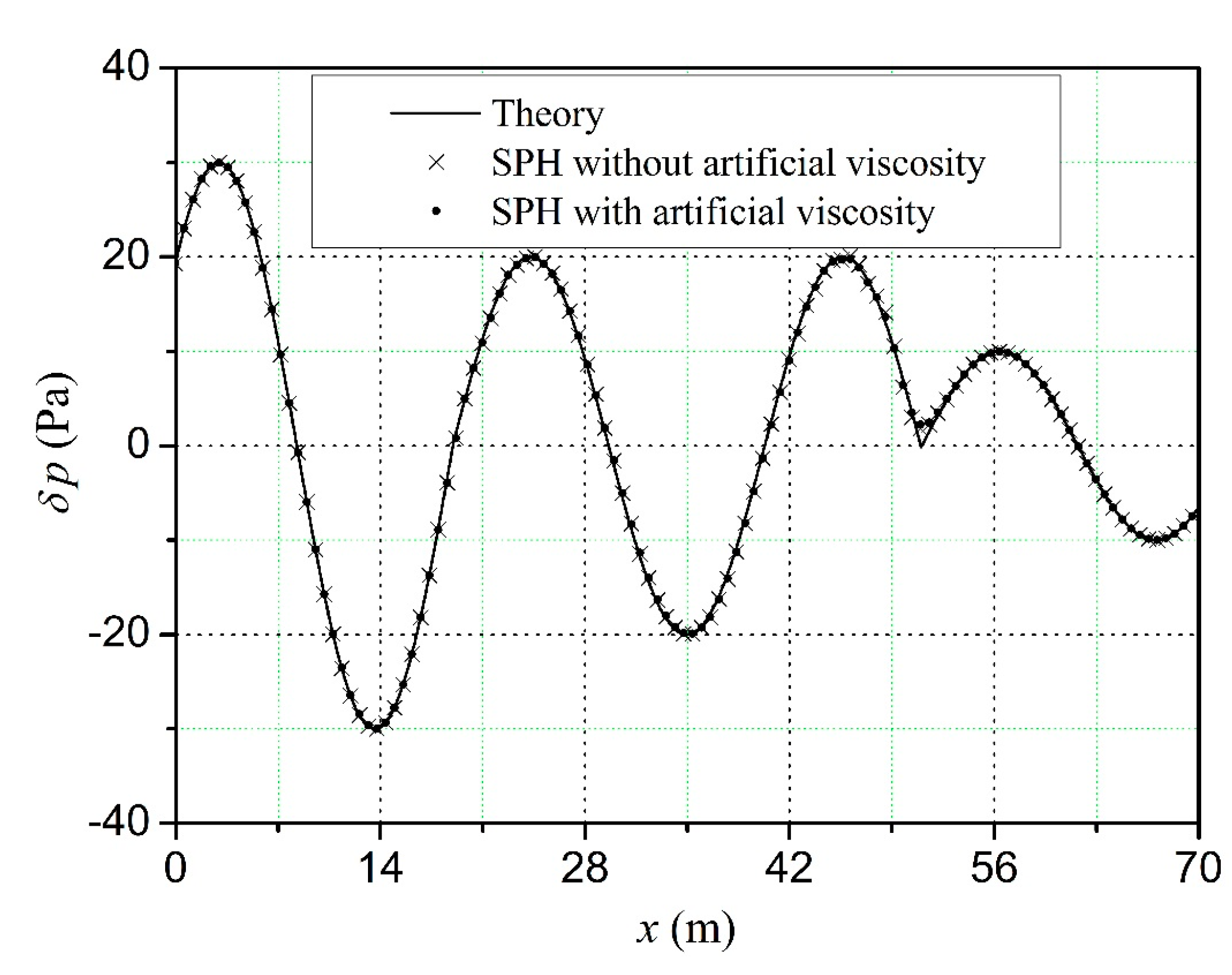
From Table 2, it can be seen that the SPH algorithms with artificial viscosity can improve the accuracy of the simulation. Compared to the sound interference simulation, when the parameters of artificial viscosity term are the same, the SPH numerical errors of sound propagation are smaller. For sound propagation, the SPH numerical errors of sound pressure reach the minimum when α_П = 0.06, β_П = 0.5. For sound interference, the SPH numerical errors of sound pressure reach the minimum when α_П = 0.03, β_П = 0.5.

Table 2. The SPH numerical errors of sound pressure.

αП	βП	Sound Propagation ɛpre (×10−4)	Sound Interference ɛpre (×10−4)
0.00	0.00	2.574247	3.674502
0.00	0.50	2.571422	3.674424
0.01	0.50	2.303623	3.615698
0.02	0.50	2.177653	3.580848
0.03	0.50	2.098490	3.565303
0.04	0.50	2.059441	3.566019
0.05	0.50	2.038529	3.580722
0.06	0.50	2.034482	3.607429
0.07	0.50	2.039658	3.644548
0.08	0.50	2.041069	3.690689

Table 2. The SPH numerical errors of sound pressure.

αП	βП	Sound Propagation ɛpre (×10−4)	Sound Interference ɛpre (×10−4)
0.00	0.00	2.574247	3.674502
0.00	0.50	2.571422	3.674424
0.01	0.50	2.303623	3.615698
0.02	0.50	2.177653	3.580848
0.03	0.50	2.098490	3.565303
0.04	0.50	2.059441	3.566019
0.05	0.50	2.038529	3.580722
0.06	0.50	2.034482	3.607429
0.07	0.50	2.039658	3.644548
0.08	0.50	2.041069	3.690689

Since sound propagation and interference are similar, we mainly discuss the effects of artificial viscosity on different sound interference models in the present work. In the discussion, different computational parameters, namely the smoothing kernel function, particle spacing and the Courant number, are considered.

Different sound interference cases with Gaussian, cubic spline and quintic spline kernel functions are simulated. The artificial viscosity terms with different values of α_П and β_П are added, and the numerical errors of sound pressure are plotted in Figure 5.

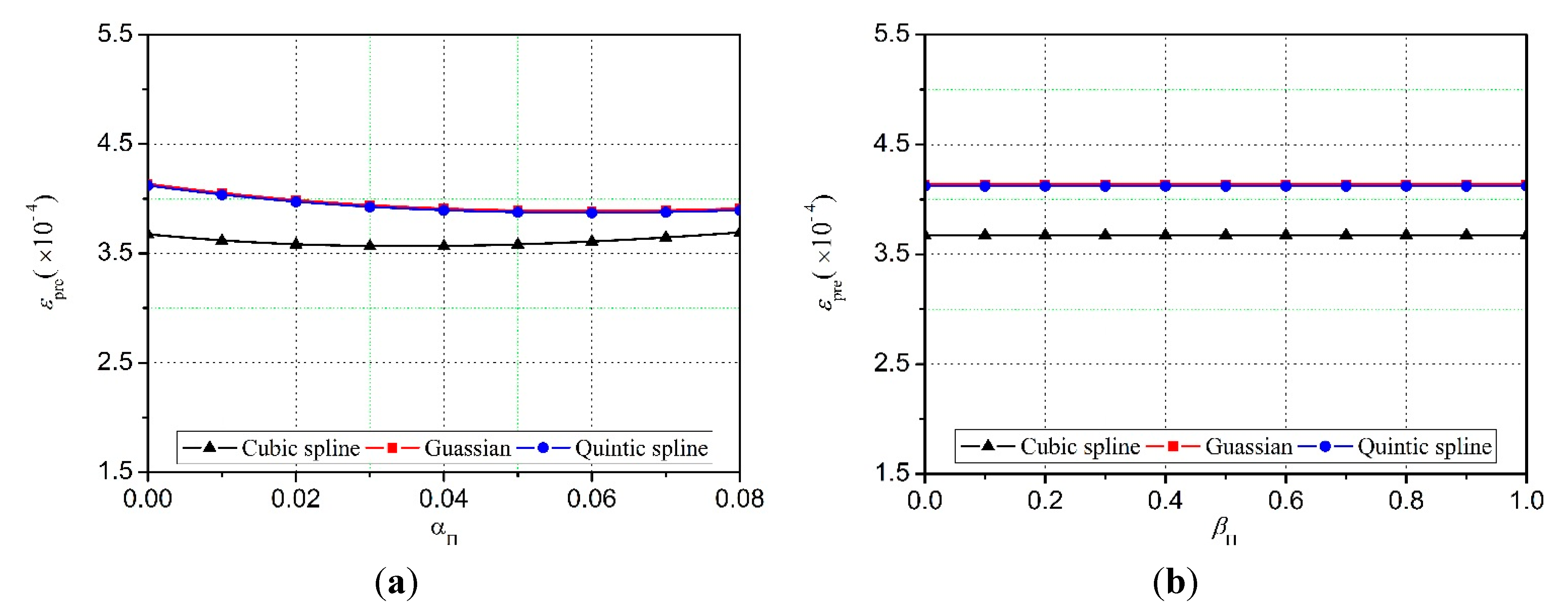
Figure 5. Numerical errors of sound pressure for sound interference models with different kinds of smoothing kernel functions. Particle spacing Δx is 0.04 m, and the Courant number is 0.04. (a) Effects of α_П on the simulation results at β_П = 0.5; (b) effects of β_П on the simulation results at α_П = 0.0.

Figure 5. Numerical errors of sound pressure for sound interference models with different kinds of smoothing kernel functions. Particle spacing Δx is 0.04 m, and the Courant number is 0.04. (a) Effects of α_П on the simulation results at β_П = 0.5; (b) effects of β_П on the simulation results at α_П = 0.0.

As shown in Figure 5, for the same particle spacing Δx and Courant number, the smoothing kernel functions have obvious effects on the SPH simulation results. The SPH simulation using the cubic spline kernel function has more accuracy results than that using the Gaussian kernel function or the quintic spline kernel function. The numerical errors of SPH simulation using the quintic spline kernel function are slightly less than those using the Gaussian kernel function, but there is not much difference between these two types.

From Figure 5a, it can be found that, for different smoothing kernel functions, adding an artificial viscosity term can reduce the numerical errors of sound pressure. The numerical errors of the SPH results with three kinds of smoothing kernel functions share a similar changing tendency with the increasing of α_П. They firstly decrease and then increase and reach their minimums when α_П locates at [0.03, 0.06]. However, as shown in Figure 5b, parameter β_П has no obvious effects on the simulation results.

The sound interference models with particle spacing ∆x separately set to 0.04 m, 0.06 m and 0.08 m are also simulated. Figure 6 shows the numerical errors of sound pressure obtained by different sound interference models.

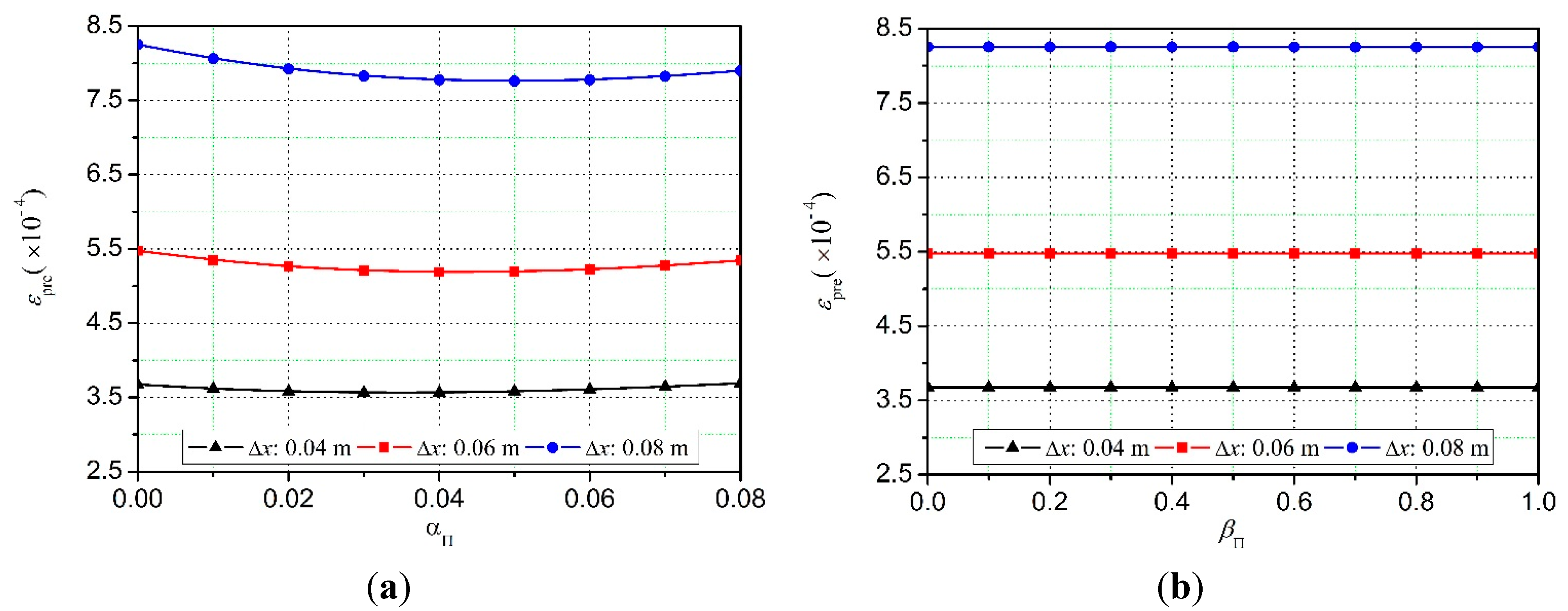
Figure 6. Numerical errors of sound pressure for sound interference models with different particle spacings. The smoothing kernel function is cubic spline, and the Courant number is 0.04. (a) Effects of α_П on the simulation results at β_П = 0.5; (b) effects of β_П on the simulation results at α_П = 0.0.

Figure 6. Numerical errors of sound pressure for sound interference models with different particle spacings. The smoothing kernel function is cubic spline, and the Courant number is 0.04. (a) Effects of α_П on the simulation results at β_П = 0.5; (b) effects of β_П on the simulation results at α_П = 0.0.

As can be seen from Figure 6, for the same smoothing kernel function and Courant number, ignoring the effect of artificial viscosity terms, the largest numerical error of sound pressure occurs when particle spacing is 0.08 m, and the least error of sound pressure happens at a particle spacing of 0.04 m. That is, the numerical errors are heavily influenced by the particle spacing Δx, and the numerical errors increase with the particle spacing increasing.

Similarly, it can also be found that the numerical errors of the SPH results with different particle spacings all have the same changing tendency with the increasing of α_П. Parameter α_П has obvious effects on the simulation results, while parameter β_П does not.

In addition, different sound interference models with Courant numbers separately set to 0.02, 0.04, 0.06 and 0.08 are simulated. Figure 7 shows the numerical errors of sound pressure for sound interference models with different Courant numbers.

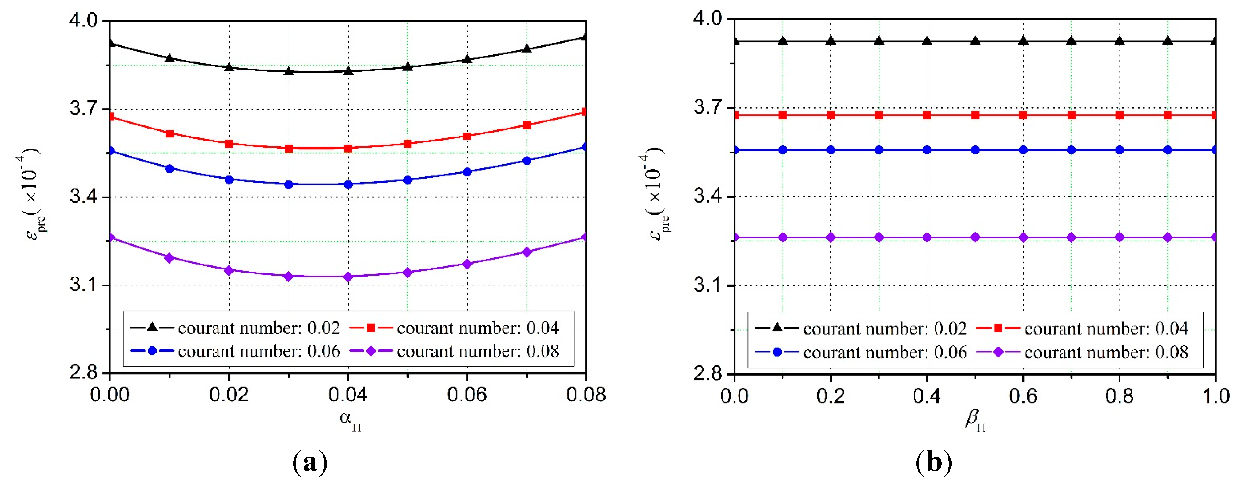
Figure 7. Numerical errors of sound pressure for sound interference models with different Courant numbers. The particle spacing Δx is 0.04 m and the smoothing kernel function is cubic spline. (a) Effects of α_П on the simulation results at β_П = 0.5; (b) effects of β_П on the simulation results at α_П = 0.0.

Figure 7. Numerical errors of sound pressure for sound interference models with different Courant numbers. The particle spacing Δx is 0.04 m and the smoothing kernel function is cubic spline. (a) Effects of α_П on the simulation results at β_П = 0.5; (b) effects of β_П on the simulation results at α_П = 0.0.

Figure 7 indicates that a better simulation result can be found when the Courant number is 0.08. For different Courant numbers, the numerical errors of sound pressure still share the same changing tendency with parameter α_П increasing. Similarly, parameter β_П has no obvious effect on the simulation results.

In summary, the SPH algorithms using the cubic spline have optimum simulation results when the particle spacing ∆x = 0.04 m and the Courant number is 0.08. The corresponding numerical errors could reach their minimum value when α_П belongs to the region [0.03, 0.06].

5. Conclusions

In this work, an artificial viscosity term is added to the standard SPH algorithm in order to improve its accuracy in modelling sound propagation and interference. SPH forms of the continuity equation, the momentum equation and the equation of state are established firstly. Following this, a one-dimensional sound propagation model and a one-dimensional sound interference model are computed to evaluate the effects of the artificial viscosity term. A comparison between SPH results with and without artificial viscosity demonstrates that a more stable and smoother simulation result can be obtained by adding an artificial viscosity term to the standard SPH algorithm, which is due to effectively reducing the unphysical oscillations. Furthermore, analysis of numerical errors of sound pressure shows that the SPH simulation using the cubic spline kernel function can obtain more accurate results with the particle spacing being 0.04 m and the Courant number being 0.08. Parameter α_П has more obvious effects than β_П on the simulation results, and the SPH algorithms of sound waves can obtain optimal results when α_П is in the region between 0.03 and 0.06, considering sound pressure error.