Processing KNN Queries in Grid-Based Sensor Networks

Department of Information Communication, Kao-Yuan University, No. 1821, Jhongshan Road, Lujhu District, Kaohsiung City 82151, Taiwan
Algorithms 2014, 7(4), 582-596; https://doi.org/10.3390/a7040582
Submission received: 10 June 2014
/
Revised: 3 October 2014
/
Accepted: 20 October 2014
/
Published: 23 October 2014
(This article belongs to the Special Issue Advanced Data Processing Algorithms in Engineering)
Abstract
:Recently, developing efficient processing techniques in spatio-temporal databases has been a much discussed topic. Many applications, such as mobile information systems, traffic control system, and geographical information systems, can benefit from efficient processing of spatio-temporal queries. In this paper, we focus on processing an important type of spatio-temporal queries, the K-nearest neighbor (KNN) queries. Different from the previous research, the locations of objects are located by the sensors which are deployed in a grid-based manner. As the positioning technique used is not the GPS technique, but the sensor network technique, this results in a greater uncertainty regarding object location. With the uncertain location information of objects, we try to develop an efficient algorithm to process the KNN queries. Moreover, we design a probability model to quantify the possibility of each object being the query result. Finally, extensive experiments are conducted to demonstrate the efficiency of the proposed algorithms.
1. Introduction
The K-nearest neighbor (KNN) query is an important type of the spatio-temproal queries. Given a set of objects So, a query object q, and a value of K, the KNN query finds the K-nearest neighbors of q among So. Previous studies [1,2,3,4,5,6] focus on processing the KNN queries on moving objects whose locations are obtained through the GPS technique. In this paper, we take the moving objects monitored by the sensor network [7,8,9] into consideration in processing the KNN queries. Two real-world examples of KNN query are presented as follows. The first example is that a fleet of warships on the sea fighting an enemy squadron. To immediately support a warship in case it is under attack, a KNN query may be used to find the friendly warships close to the warship requiring to be supported. The second example is that a traveler planning a trip from city A to city B. In this scenario, the traveler can issue a KNN query to find the nearest hotels during the trip.
For each moving object tackled in this paper, its location cannot be obtained through the GPS technique. Instead, the moving object is monitored by taking advantage of another positioning technique, the sensor-based tracking system. As the location of each object is determined by the sensor network, the uncertainty of the object’s location is much higher than that of object monitored by the GPS technique. This would incur a higher cost of processing the KNN queries. In the following, we will discuss the difficulties that need to be addressed in processing the KNN queries.
The first difficulty is how to quantify the uncertainty of moving objects. As the moving objects are monitored in the sensor network, the uncertainty of objects is dominated by the number of sensors. Due to the limited number of sensors, different deployment strategies for the sensor network will result in different uncertainty of object locations. As such, developing an appropriate sensor deployment is important to effectively reduce the uncertainty of object locations.
The second difficulty is how to develop an efficient index for managing the objects moving in the sensor network. The existing index structures are well-designed for the moving objects that have precise location information. In this paper, we consider the moving objects with uncertainty when the KNN query is processed. Therefore, a new index structure is needed to manage such moving objects.
The third difficulty is how to design an efficient KNN query processing algorithm to find the K-nearest neighbors of the query object. Due to the movement of objects, the query result would change with time (that is, the query result is dependent on the current location of the query object). This makes the execution of the KNN query more complicated. We will discuss the characteristic of the KNN query so as to develop the query processing algorithm with better performance.
The last difficulty is how to reasonably give each moving object a probability of being the K-nearest neighbor (i.e., the probability of object being the query result). As the objects move with uncertain location, there exist some objects that are possible to be the K-nearest neighbor (that is, these objects are possible answers for the KNN query). When the number of possible answers increases, the situation becomes very hard to choose the most appropriate objects. Therefore, a probability model must be built to reasonably provide probabilistic answers to the KNN query.
The main contributions of this paper are summarized as follows.
- An efficient sensor deployment strategy is used to construct the sensor network.
- An effective mechanism is designed to quantify the uncertainty of objects moving in such a sensor network.
- A grid index with update operations is developed to manage moving objects in the sensor network.
- A query processing algorithm is developed to efficiently answer the KNN query. Also, a reasonable probability is designed to quantify the possibility of each object being the query result.
- A comprehensive set of experiments is conducted to evaluate the efficiency of the proposed methods.
The remainder of this paper is organized as follows. In Section 2, the uncertain model is introduced. Section 3 describes the grid index used in query processing. In Section 4, we present the proposed algorithm for answering the KNN query. Section 5 presents the designed probability model. Section 6 shows the performance evaluation. In Section 7, we discuss some related work in processing the spatio-temporal queries. Finally, Section 8 concludes this paper.
2. Uncertain Model
To monitor the moving object, we need to design a sensor deployment to construct the sensor network. In the constructed sensor network, each object moves with uncertain location as time progresses. In the following, we introduce the sensor deployment strategy, and then present the uncertain model for the moving objects.
2.1. Sensor Deployment
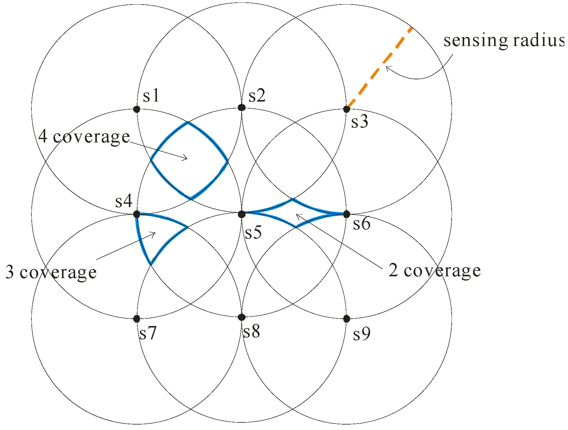
Different sensor deployment strategies would result in different covering regions of sensor network, which incurs a significant difference between the uncertainties of objects’ locations. To effectively reduce the cost of constructing the sensor network, we apply a grid deployment strategy to build the sensor network. Let us use Figure 1 to illustrate the grid deployment. In this example, the sensor network is constructed by 9 sensors. As each sensor has the same sensing radius r, the distance between each sensor is equal to r. It is easy to implement a grid-based sensor network, and thus the constructing cost can be effectively reduced.
As the sensing technique of the sensor network cannot precisely monitor the moving objects, the locations of objects in the sensor network are uncertain. As for the uncertain extent of each object, it is dependent on the covering region of sensor network. Using the above grid deployment, each object is monitored by at least two sensors (i.e., 2 coverage), and is monitored by at most four sensors (i.e., 4 coverage). That is, each object belongs to one of the following cases: 2 coverage, 3 coverage and 4 coverage (depicted as the blue regions shown in Figure 1).
Figure 1.
Grid deployment.

2.2. Object Uncertainty
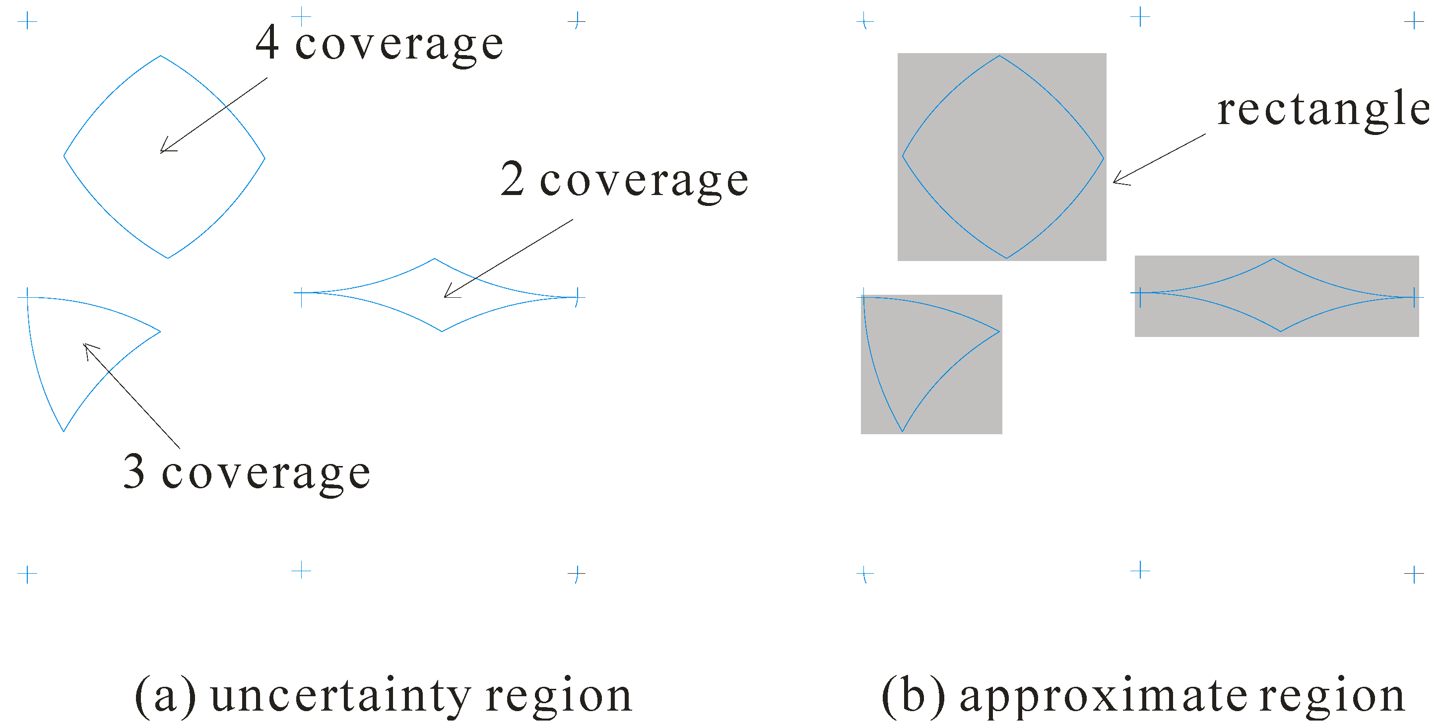
For each object, it is monitored by at least two sensors. However, due to the inherent uncertain property of sensors, the objects are imprecisely tracked. That is, we can know the possible locations of each object, instead of its precise location. Let us consider again the example in Figure 1. For the 2 coverage region monitored by the sensor 5 and the sensor 6, all the points inside it could be the actual location of object. Similarly, the 3 and 4 coverage regions represent the possible locations of the object. We term the coverage regions the uncertainty regions.
When the KNN query is processed, different locations of object would result in different query results. As such, all the points inside the uncertainty region need to be considered in processing the KNN query. However, as we can see from Figure 2a, the shape of the uncertainty regions (including the 2, 3, and 4 coverage regions) is irregular, which makes it hard to quantify the uncertainty of object. As a result, we adopt a minimum rectangle to enclose the uncertainty region as shown in Figure 2b, and utilize it to approximate the uncertainty region in query processing. We term the minimum bounding rectangle the approximate region.
Figure 2.
Uncertainty model.

3. Index Structure
To efficiently manage the objects moving in the sensor network, a well-designed index structure is required. However, the uncertainty on object locations makes the design and the maintenance of index structure much harder. In this section, we design a grid index to store the location information of the objects. In the following, we first describe the designed grid index. Then, we illustrate how to manage the objects using the grid index.
3.1. Grid Index
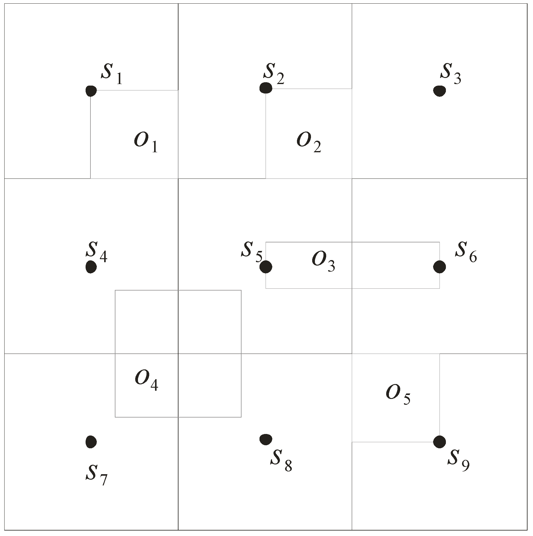
In our model, the uncertainty of objects’ locations is represented as an approximate region with rectangular shape. We use a grid index to efficiently manage the approximate regions. The data space is first divided into N*N grid cells, and then each grid cell stores information of the objects, and the sensor inside it. Consider the example in Figure 3. There are five objects o1 to o5 moving in the sensor network. The entire space of network is divided into 3*3 grid cells and monitored by nine sensors s1 to s9. That is, each sensor is located at the center of a grid cell and responsible for monitoring this cell. In the sequel, we describe the data structures used for storing information of the sensors and the objects.
Figure 3.
Grid index.
3.2. Data Structures
Two tables, To and Ts, are used to keep the information of grid index. The first table To stores the information of the objects in the sensor network. The information contains (1) o-id: the object id; (2) s-list: the sensors that monitor this object currently; (3) tc: the time point at which this object begins to be monitored; and (4) o-data: the basic data of this object (such as age, height, and weight). The second table Ts keeps the information of the sensors. The information is (1) s-id: the sensor id; (2) s-radius: the sensing radius of this sensor; and (3) o-list: the objects monitored by this sensor.
3.3. Index Updates
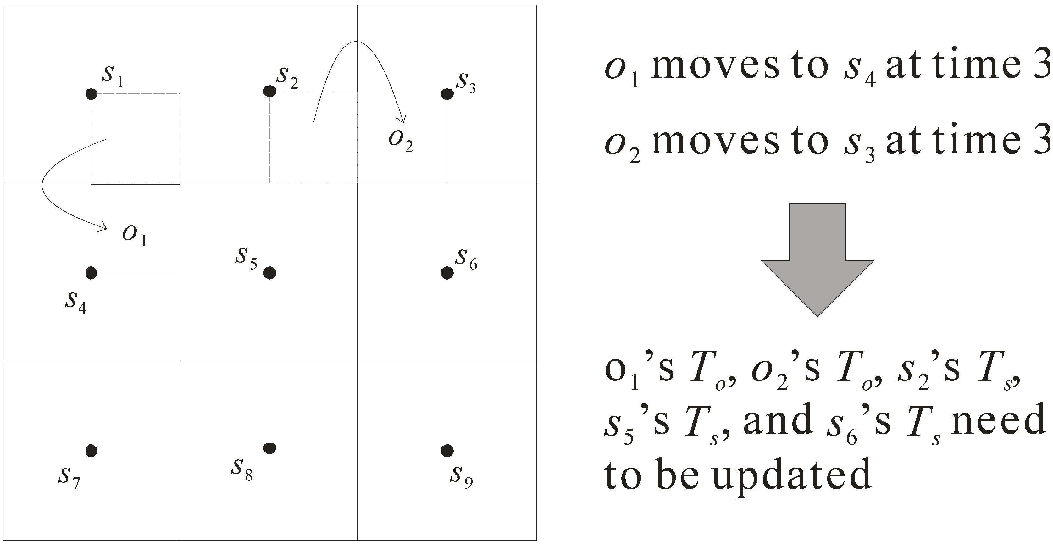
As the objects in the sensor network move with time, the grid index needs to be updated so as to precisely store the object information. Here, we design an efficient mechanism to rapidly update the location information of objects. Consider the example in Figure 4, which shows how to process the updates of objects. In this example, at time 3, objects o1 and o2 move from the regions monitored by sensors s1 and s2 to the regions monitored by sensors s4 and s3, respectively. Due to the movement of objects o1 and o2, the following five tables of grid index need to be updated.
- Updating To of object o1: when o1 moves, sensor s2 cannot monitor o1 while sensor s5 begins to monitor o1. Therefore, its table To is changed from (o1, {s1, s2, s4}, 0, o1-data) to (o1, {s1, s4, s5}, 3, o1-data).
- Updating To of object o2: once o2 moves, sensor s5 cannot monitor o2 but s6 can monitor o2. As such, the table To is updated from (o2, {s2, s3, s5}, 0, o2-data) to (o2, {s2, s3, s6}, 3, o2-data).
- Updating Ts of sensor s2: due to the movement of o1, the table Ts of s2 needs to be updated. It is changed from (s2, 60, {o1, o2}) to (s2, 60, {o2}).
- Updating Ts of sensor s5: because the locations of o1 and o2 are changed, the table Ts of s5 needs to be updated. It is changed from (s5, 60, {o2}) to (s5, 60, {o1}).
- Updating Ts of sensor s6: as object o2 moves, sensor s6’s table Ts is updated. It is changed from (s6, 60, {null}) to (s6, 60, {o2}).
Figure 4.
Update mechanism.

4. Query Processing Algorithm
In this paper, we focus on processing the KNN query for moving objects in the grid-based sensor network. Given a sensor s issuing the query and a value of K, the KNN query retrieves the K-nearest neighbors of s. We develop an efficient algorithm combined with the grid index to answer the KNN query. In the following, we first define the parameters used to prune the non-qualifying objects and then illustrate the detailed steps of the algorithm. For ease of explanation, we assume that the 1NN query is processed (i.e., K = 1).
4.1. Parameters and Pruning Criteria
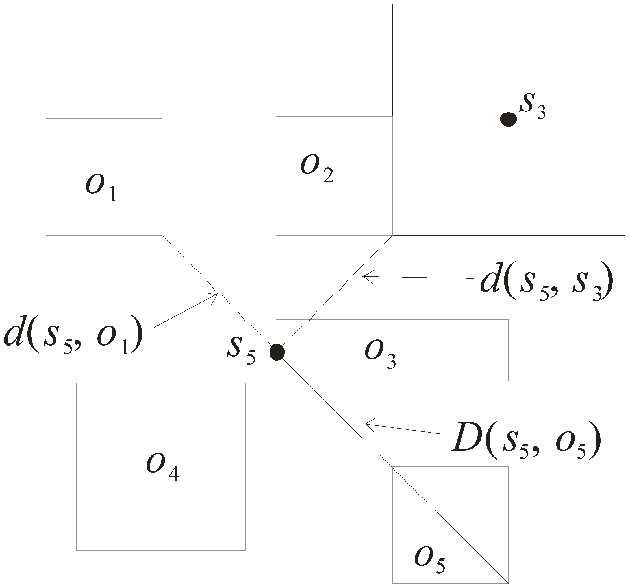
Three parameters are used to design the pruning criteria. They are d(s, o), D(s, o), and d(s, s’), which are described as follows.
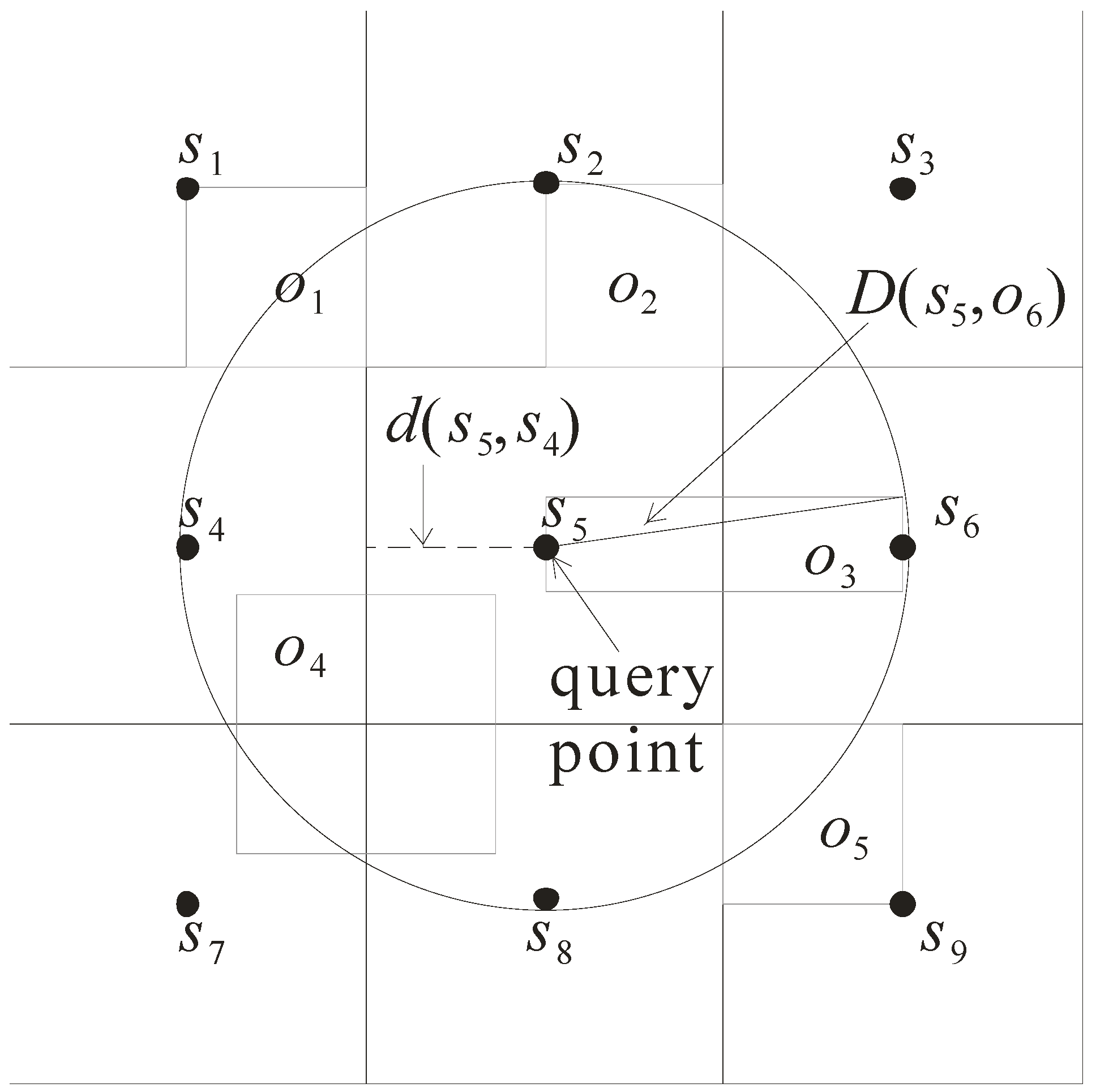
- Distance d(s, o): it refers to the minimal distance between the sensor s and the approximate region of object o. As shown in Figure 5, d(s5, o1) is the minimal distance of the sensor s5 to the approximate region of o1. Note that the minimal distance d(s5, o3) is equal to 0 as s5 is enclosed in the approximate region of o3.
- Distance D(s, o): it refers to the maximal distance between the sensor s and the approximate region of object o. Consider again the example in Figure 5. D(s5, o5) is the maximal distance between the sensor s5 and the approximate region o5.
- Distance d(s, s’): it refers to the minimal distance from the sensor s to the grid cell monitored by the sensor s’. For example, d(s5, s3) is the minimal distance between s5 and the grid cell monitored by s3.
Having defined the three parameters, we develop the following pruning criteria to efficiently prune the objects that are impossible to be the KNN results.
- Pruning criterion 1: if the maximal distance D(s, o) of sensor s to object o is less than the minimal distance d(s, o’) of sensor s to object o’, then o’ cannot be the NN and thus is pruned.
- Pruning criterion 2: if the maximal distance D(s, o) of sensor s to object o is less than the minimal distance d(s, s’) of sensor s to the grid cell monitored by another sensor s’, then the objects monitored by sensor s’ can be pruned as their distances to sensor s must be greater than that of object o.
Figure 5.
Illustration of parameters.

4.2. Detailed Steps
The query processing algorithm consists of three steps. Here, we describe them as follows.
- Step 1: starting from the grid cell monitored by the sensor s issuing the query, each grid cell is visited according to its distance to the sensor s. When a grid cell is visited, d(s, o) and D(s, o) of objects enclosed by this grid cell are computed. This step proceeds until d(s, s’) of the visited grid cell is greater than D(s, o) of an object. That is, all the unvisited cells are pruned.
- Step 2: sorting D(s, o) of the objects kept from Step 1 so as to derive a smallest D(s, o), defined as the pruning distance. For each object, if its d(s, o) is greater than the pruning distance, then it can be pruned. As such, in this step, d(s, o) of each object is compared against the pruning distance. Only the objects whose d(s, o) is less than or equal to the pruning distance are kept for the next step.
- Step 3: for each object kept from Step 2, its probability of being the query result is computed (which will be discussed later).
        Algorithm 1: Query Processing Algorithm

        Input: A sensor s issuing the query and a value of K
        Output: The K-nearest neighbors of s

        foreach grid cell monitored by sensor s’ do
          compute d(s, s’);
          if d(s, s’) ≤ D(s, o) of K objects then
            compute d(s, o) and D(s, o) of objects enclosed by the grid cell and insert the objects into set O;
        sort objects in O in ascending order of D(s, o) and set pruning distance to K-th smallest D(s, o);
        foreach object o є O do
          if D(s, o) is greater than the pruning distance then remove o from O;
        foreach object o є O do compute its probability;
        return the K objects with highest probabilities.
Let us use Figure 6 to illustrate how the query processing algorithm works. Assume that the sensor s5 issues the NN query. The network expansion starts from the grid cell monitored by sensor s5. As the object o3 is monitored by s5, its d(s5, o3) and D(s5, o3) are computed. Then, the grid cells monitored by the other eight sensors are visited because their d(s5, s’) is less than D(s5, o3). When Step 1 is finished, objects o1 to o5 are kept with their distances d(s5, o) and D(s5, o). By comparing the distance D(s5, o) of objects o1 to o5, the pruning distance is set to D(s5, o3). As the distance d(s5, o) of each object is less than or equal to the pruning distance, it is possible to be the NN. Thus, objects o1 to o5 are kept for executing Step 3.
Figure 6.
Example of K-nearest neighbor (KNN) query.
5. Probability Model
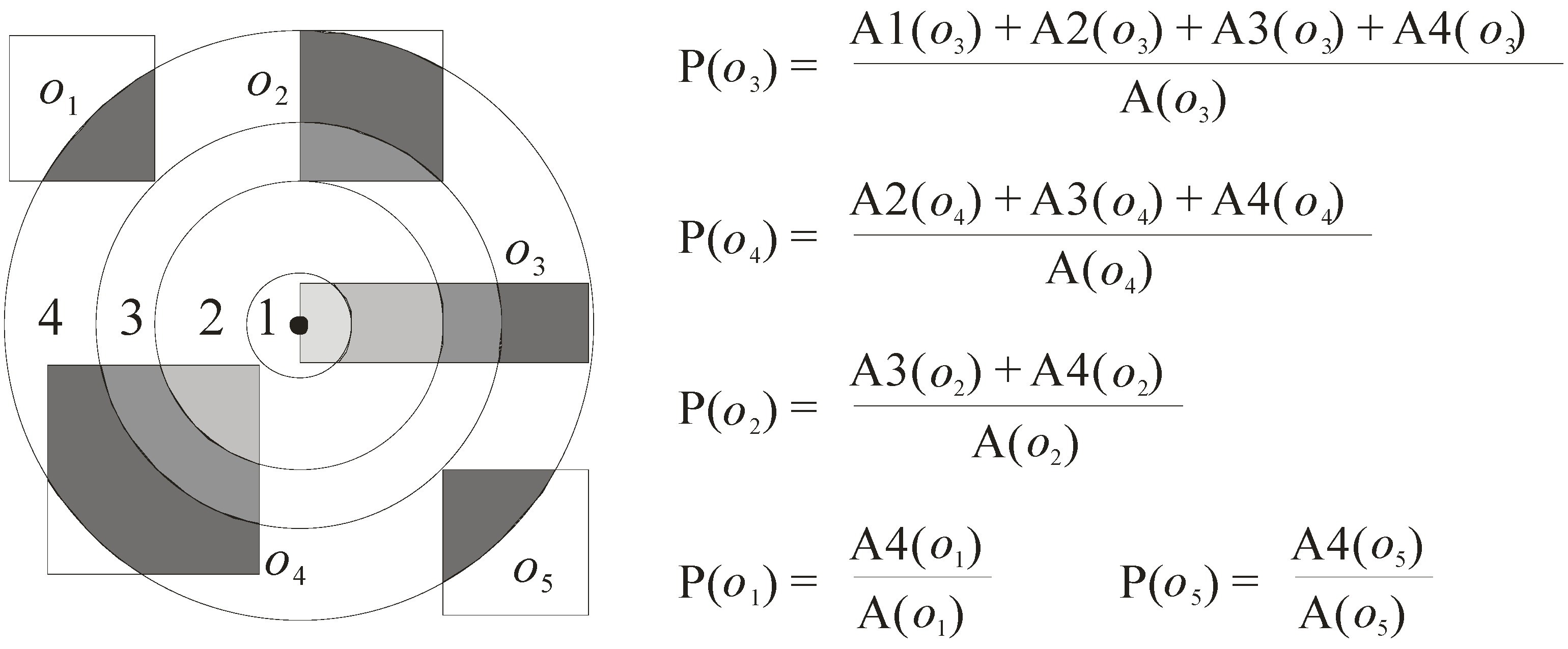
The probability model is designed to reasonably give each object a probability that quantifies the possibility of being the query result. Based on the probability, the server can provide more useful information for the user to decide the most appropriate result. The following parameter, P(o), is designed to compute the probability of the object o being the query result.
- P(o) = (A1(o) + A2(o) + … + An(o))/A(o), where Ai(o) (1 ≤ i ≤ n) is the area of the ith region of object o that overlaps the circle whose radius is equal to the length of the pruning distance (here, the circle is denoted as C), and A(o) refers to the area of the approximate region of object o.
Let us use Figure 7, which continues the example in Figure 6, to illustrate how the probabilities of the objects are computed. In this example, the probabilities of the five objects o1 to o5 are computed. For the object o3, as there are four regions A1(o3), A2(o3), A3(o3), and A4(o3) that overlap the circle C, its probability P(o3) is computed as (A1(o3) + A2(o3) + A3(o3) + A4(o3))/A(o3). The probabilities of the other four objects o1, o2, o4, and o5 can be computed in a similar way. The final result is also shown in Figure 7.
6. Performance Evaluation
We conduct several experiments for the proposed algorithm in this section. We evaluate the performance by considering the CPU time and the number of accessed grid cells for processing the KNN query under various important parameters.
Figure 7.
Probability calculation.

6.1. Experimental Settings
All experiments are performed on a PC with AMD Athlon 64 X2 5200 CPU and 2GB RAM. The algorithms are implemented in C++. In the simulation, 128 × 128 sensors are used to construct the sensor network, in which objects (varying from 0.1 K to 200 K) would change their locations after every Tu time units. In the experimental space, we also randomly generate 30 query points. Each of these query points issues a KNN query, where the default value of K is set to 10. The performance is measured by the average CPU time and the average number of accessed cells in performing workloads of the 30 queries. We compare the proposed algorithm (termed as KNN) with a PNNQ approach (termed as PNNQ) [10] which is performed without the grid index support. Table 1 summarizes the parameters under investigation, along with their default values and ranges.

| Parameter | Default | Range |
|---|---|---|
| Object distribution | uniform | uniform, Gaussian, zipf |
| Object number (K) | 100 | 0.1, 1, 10, 100, 200 |
| Tu | 15 | 5, 10, 15, 20, 25 |
| K | 10 | 1, 5, 10, 15, 20 |
6.2. Efficiency Evaluation
In this subsection, we measure the performance of the proposed KNN algorithm and the PNNQ approach in terms of the CPU time and the number of accessed cells of grid index. Four experiments are conducted to investigate the effects of four important factors on the performance of processing the KNN query. These important factors include the distribution of objects, the number of object, the time Tu at which object changes its location, and the value of K.
The first experiment studies how the distribution of objects affects the performance of KNN and PNNQ by considering three types of object distributions. These object distributions are the uniform distribution, the Gaussian distribution (with variance 0.05 and a mean being the coordinate of the center), and the Zipf distribution (with skew coefficient 0.8). Note that hereafter all figures use a logarithmic scale for the y-axis. As shown in Figure 8a, the CPU time of both approaches for the uniform distribution is slightly lower than that for the Gaussian and Zipf distributions. This is because for the Gaussian and Zipf distributions, the objects are closer to each other (compared to the uniform distribution) so that more CPU time is required to find the KNN result. As for the number of accessed cells, Figure 8b indicates that when the objects follow the Zipf distribution, the KNN approach requires a little more accessed cells (comparing to the uniform and Gaussian distributions). For the PNNQ approach, the number of accessed cells remains constant regardless of the object distribution. The main reason is that PNNQ is performed without the grid index support so that all the grid cells need to be accessed. From the above experimental results, we know that the KNN approach significantly outperforms the PNNQ approach.
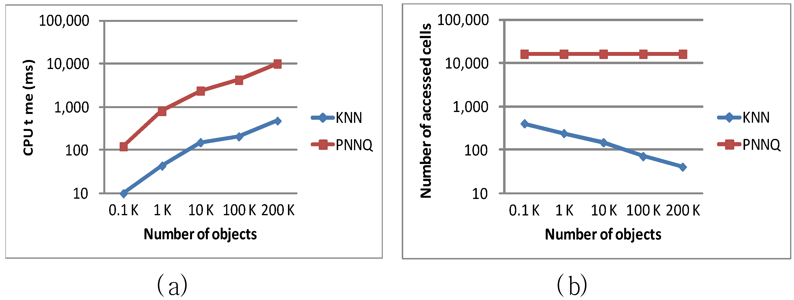
Figure 9 illustrates the performance of the KNN and PNNQ approaches as a function of the number of objects (ranging from 0.1 K to 200 K), in terms of the CPU overhead and the number of accessed cells. As shown in Figure 9a, the CPU time for both approaches increases with the increase of object number because more distance computations of objects are required for finding the KNN result. Nevertheless, the KNN approach significantly outperforms the PNNQ approach in all cases. This is mainly because for the PNNQ approach the distances of all objects have to be computed which incurs high computation cost as the object number increases, whereas for the KNN approach the unnecessary distance computation of these objects can be avoided by applying the designed pruning criteria and the support of grid index. The experimental result in Figure 9b illustrates that the number of accessed for the PNNQ approach remains constant in all cases. This is because no matter what the object quantity is, for the PNNQ approach all cells need to be accessed. An interesting observation from Figure 9b is that a larger number of objects results in a lower number of cells that need to be accessed in processing the KNN query. The main reason is that when the sensor network is sparse (e.g., object number is 0.1 K or 1 K), more cells have to be accessed so as to find the Kth NN, while a dense network (e.g., object number is 200 K) may lead to early termination of finding the Kth NN so that fewer cells are accessed.
Figure 8.
Effect of object distribution.
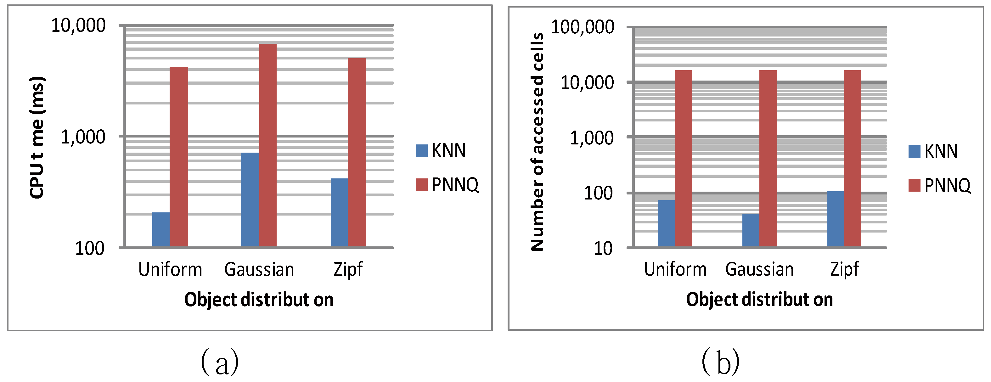
Figure 9.
Effect of number of objects.

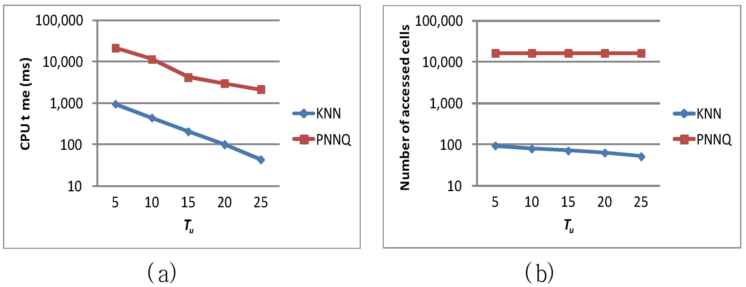
In the following, we demonstrate the efficiency of the proposed algorithm by studying the effect of the update interval (i.e., the value of Tu) on the query performance. Figure 10a and Figure 10b investigate the impacts of various update intervals (i.e., varying Tu) on the CPU time and the number of accessed cells for the proposed approaches (that is, the KNN approach and the PNNQ approach), respectively. In the experiments, we vary Tu from 5 to 25 time units and measure the performance for the two approaches. As shown in Figure 10a, for the larger Tu (e.g., Tu = 20 or 25 time units), the frequency of object’s location being changed is lower so that the degradation of the CPU time for the PNNQ approach is not significant. However, as Tu decreases (i.e., more location changes occur), the PNNQ approach performs significantly worse than the KNN approach. In Figure 10b, we measure the number of accessed cells for the KNN and PNNQ approaches as a function of Tu. The experimental result shows that the number of accessed cells is basically constant for different Tu, which implies that the performance of the proposed approaches is insensitive to the value of Tu. The result also confirms again that applying the KNN approach can greatly improve the performance of processing the KNN query.
Figure 10.
Effect of Tu.

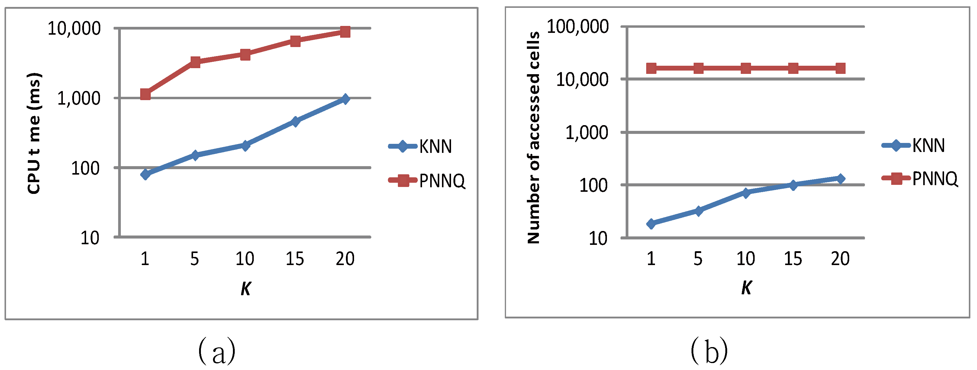
The last experiment evaluates the effect of the number of nearest neighbors (i.e., K) on the CPU time and the number of accessed cells of the KNN approach and the PNNQ approach. As shown in Figure 11a, when the value of K increases, the CPU overhead for both the KNN approach and the PNNQ approach grows. The reason is that as K becomes greater, the number of qualifying objects inevitably increases so that more distance computations of these objects are required. Nevertheless, in terms of CPU time, the KNN approach outperforms the PNNQ approach by a factor of up 10 in all cases. As for the effect of K on the number of accessed cells shown in Figure 11b, the curve for the KNN (PNNQ) approach has the increasing (constant) trend. The increasing trend for the KNN approach is because as K increases, the Kth NN becomes farther from the query point and hence more cells would be accessed. Nevertheless, the KNN approach reduces the number of accessed cells by almost two orders of magnitude compared to the PNNQ approach.
Figure 11.
Effect of K.

7. Related Work
Sistla et al. [11] first identify the importance of the spatio-temporal queries and describe modeling methods and query languages for the expression of these queries. They further attempt to build a database of moving objects, called the DOMINO [12], on top of existing DBMS. The main focus of DOMINO is to support new kinds of spatio-temporal attributes and query language for moving objects. However, the issues of processing the spatio-temporal queries are not exclusively addressed by the above works. Recently, several methods have been designed to efficiently process the spatio-temporal queries over moving objects.
Kalashnikov et al. [3] propose a method operated with R-tree and Quadtree to efficiently process range query. Tao et al. [4] propose a repetitive query processing approach with a TPR-tree for answering the range and KNN queries. Benetis et al. [13] develop an approach to find the nearest neighbor through a depth-first traversal of TPR-tree. To adapt to moving objects and reduce computational cost, Raptopoulou et al. [14] propose efficient methods that process the KNN query by tracing the change of the Kth NN. Iwerks et al. [15] answer a KNN query through a method that a range query is first processed and then KNN result are determined among the objects qualifying the range query. If the number of objects that satisfy the range query is greater than K, the answer to KNN query can be obtained from these objects. Song et al. [16] propose an approach in which the snapshot KNN query is re-evaluated at each time instant. Their approach is restricted in processing the KNN query over static objects. Nehme et al. [17] extend the approach in [16] to adapt to moving object datasets. They utilize the concepts of shared execution and incremental evaluation to process range query on moving objects. Recently, the technique of incremental evaluation has been further adopted by Mouratidis et al. [6], Xiong et al. [18] and Yu et al. [19] to answer the KNN query.
The above KNN methods are developed for the moving objects, in which the locations of objects are obtained through the GPS technique, instead of the sensor network technique. Moreover, all the mentioned methods focus on processing the KNN query under the situation that moving objects have precise locations. This means that these methods are inapplicable to the KNN query with uncertainty as proposed in this paper (where a probabilistic method is needed). Cheng et al. [10] propose a PNNQ approach for processing the KNN query over objects with uncertainty, which is similar to the problem tackled in this paper. However, there are significant differences compared to our work, which are described as follows: (1) the uncertainty model in [10] is a circle or a line segment; (2) no grid index is used in [10]; and (3) the probability model in [10] is based on numerical integration.
8. Conclusions
In recent years, many studies focused on query processing techniques in spatio-temporal databases. In this paper, we tried to apply the query processing techniques to the environment of sensor network, in which objects are monitored by sensors and move with uncertainty. We first designed an effective mechanism to quantify the uncertainty of the objects moving in the sensor network. Then, we developed a grid index to efficiently manage the objects with uncertainty. We also proposed an efficient algorithm to answer the KNN query. Finally, a reasonable probability model was designed to quantify the possibility of each object being the query result.
Acknowledgments
This work was supported by National Science Council of Taiwan (R.O.C.) under Grants NSC102-2119-M-244-001 and MOST103-2119-M-244-001.
Conflicts of Interest
The authors declare no conflict of interest.
References
- Zhang, J.; Zhu, M.; Papadias, D.; Tao, Y.; Lee, D.L. Location-based Spatial Queries. In Proceedings of the 2003 ACM SIGMOD international conference on Management of data, San Diego, CA, USA, 9–12 June 2003; pp. 443–454.
- Saltenis, S.; Jensen, C.S.; Leutenegger, S.T.; Lopez, M.A. Indexing the Positions of Continuously Moving Objects; ACM SIGMOD: Dallas, TX, USA, 2000. [Google Scholar]
- Kalashnikov, D.V.; Prabhakar, S.; Hambrusch, S.; Aref, W. Efficient evaluation of continuous range queries on moving objects. In Proceedings of the International Conference on Database and Expert Systems Applications, Aix en, France, 2–6 September 2002; pp. 731–740.
- Tao, Y.; Papadias, D. Time Parameterized Queries in Spatio-Temporal Databases. In Proceedings of the 2002 ACM SIGMOD international conference on Management of data, Madison, WI, USA, 3–6 June 2002; pp. 322–333.
- Mokbel, M.F.; Xiong, X.; Aref, W.G. Sina: Scalable Incremental Processing of Continuous Queries in Spatio-Temporal Databases. In Proceedings of the 2004 ACM SIGMOD international conference on Management of data, Paris, France, 13–18 June 2004; pp. 623–634.
- Mouratidis, K.; Hadjieleftheriou, M.; Papadias, D. Conceptual Partitioning: An Efficient Method for Continuous Nearest Neighbor Monitoring. In proceedings of the 2005 ACM SIGMOD international conference on Management of data, Baltimore, MD, USA, 14–16 June 2005; pp. 634–645.
- Jung, C.; Lee, S.J.; Bhuse, V. The minimum scheduling time for convergecast in wireless sensor networks. Algorithms 2014, 7, 145–165. [Google Scholar] [CrossRef]
- Ma, W.; Zhang, J. Algorithm based on heuristic strategy to infer lossy links in wireless sensor networks. Algorithms 2014, 7, 397–404. [Google Scholar] [CrossRef]
- Nikoletseas, S.; Spirakis, P.G. Probabilistic distributed algorithms for energy efficient routing and tracking in wireless sensor networks. Algorithms 2009, 2, 121–157. [Google Scholar] [CrossRef]
- Cheng, R.; Kalashnikov, D.V.; Prabhakar, S. Querying Imprecise Data in Moving Object Environments. IEEE Trans. Knowl. Data Eng. 2009, 16, 1112–1127. [Google Scholar] [CrossRef]
- Sistla, A.P.; Wolfson, O.; Chamberlain, S.; Dao, S. Modeling and Querying Moving Objects. In Proceedings of the International Conference on Data Engineering, Birmingham, UK, 7–11 April 1997; pp. 422–432.
- Wolfson, O.; Sistla, P.; Xu, B.; Zhou, J.; Chamberlain, S.; Yesha, T.; Rishe, N. Tracking Moving Objects Using Database Technology in DOMINO. In Proceedings of the Fourth Workshop on Next Generation Information Technologies and Systems, Zikhron-Yaakov, Israel, 5–7 July 1999.
- Benetis, R.; Jensen, C.S.; Karciauskas, G.; Saltenis, S. Nearest Neighbor and Reverse Nearest Neighbor Queries for Moving Objects. In Proceedings of the International Database Engineering and Applications Symposium, Edmonton, Canada, 17–19 July 2002; pp. 44–53.
- Raptopoulou, K.; Papadopoulos, A.N.; Manolopoulos, Y. Fast Nearest-Neighbor Query Processing in Moving-Object Databases. GeoInformatica 2003, 7, 113–137. [Google Scholar] [CrossRef]
- Iwerks, G.; Samet, H.; Smith, K. Continuous K-Nearest Neighbor Queries for Continuously Moving Points with Updates. In Proceedings of the International Conference on Very Large Data Bases, Berlin, Germany, 9–12 September 2003; pp. 512–523.
- Song, Z.; Roussopoulos, N. K-Nearest Neighbor Search for Moving Query Point. In Proceedings of 7th International Symposium on Advances in Spatial and Temporal Databases, Redondo Beach, CA, USA, 12–15 July 2001; pp. 79–96.
- Nehme, R.V.; Rundensteiner, E.A. SCUBA: Scalable Cluster-Based Algorithm for Evaluating Continuous Spatio-Temporal Queries on Moving Objects. In Proceedings of the 10th International Conference on Extending Database Technology, Munich, Germany, 26–31 March 2006; pp. 1001–1019.
- Xiong, X.; Mokbel, M.F.; Aref, W.G. SEA-CNN: Scalable Processing of Continuous K-Nearest Neighbor Queries in Spatio-temporal Databases. In Proceedings of the International Conference on Data Engineering, Tokyo, Japan, 5–8 April 2005; pp. 643–654.
- Yu, X.; Pu, K.Q.; Koudas, N. Monitoring K-Nearest Neighbor Queries Over Moving Objects. In Proceedings of the International Conference on Data Engineering, Tokyo, Japan, 5–8 April 2005; pp. 631–642.
© 2014 by the authors; licensee MDPI, Basel, Switzerland. This article is an open access article distributed under the terms and conditions of the Creative Commons Attribution license (http://creativecommons.org/licenses/by/4.0/).
Share and Cite
MDPI and ACS Style
Huang, Y.-K. Processing KNN Queries in Grid-Based Sensor Networks. Algorithms 2014, 7, 582-596. https://doi.org/10.3390/a7040582
AMA Style
Huang Y-K. Processing KNN Queries in Grid-Based Sensor Networks. Algorithms. 2014; 7(4):582-596. https://doi.org/10.3390/a7040582
Chicago/Turabian StyleHuang, Yuan-Ko. 2014. "Processing KNN Queries in Grid-Based Sensor Networks" Algorithms 7, no. 4: 582-596. https://doi.org/10.3390/a7040582