Algorithm Based on Heuristic Strategy to Infer Lossy Links in Wireless Sensor Networks

Abstract
:1. Introduction
2. Network Model
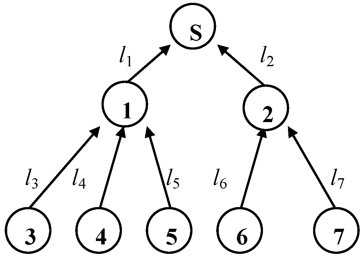
2.1. Topology Model

2.2. Performance Model
3. Inference Algorithm
3.1. Problem Description
3.2. Algorithm Description
4. Simulation and Evaluation


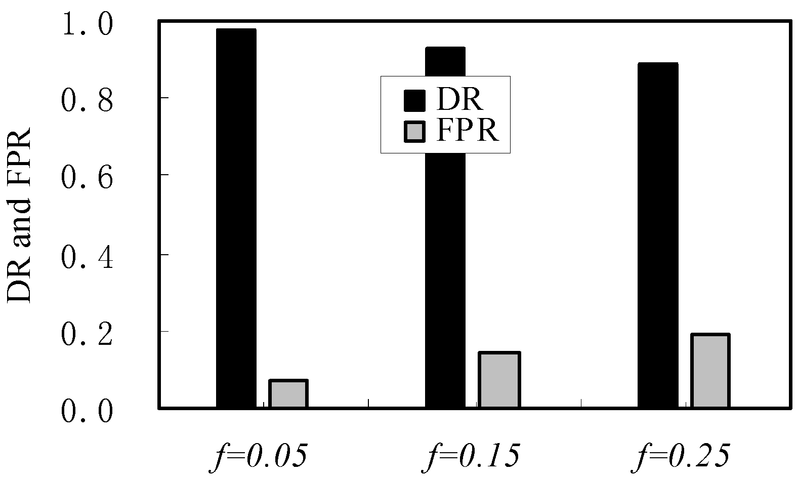
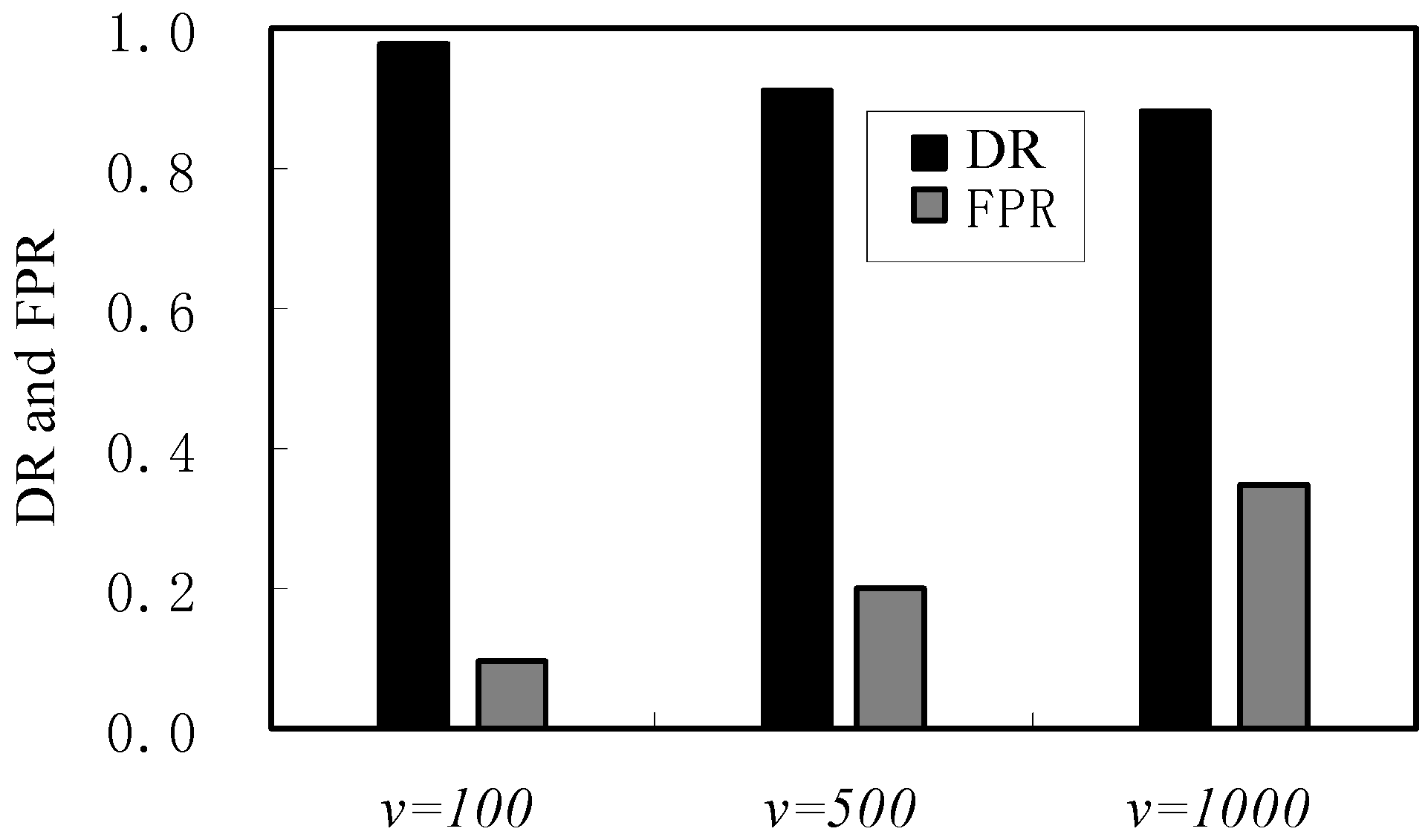
| Performance | f = 0.05 | v = 100 | f = 0.15 | v = 500 | f = 0.25 | v = 1000 |
|---|---|---|---|---|---|---|
| HLLI | SCFS | HLLI | SCFS | HLLI | SCFS | |
| DR/(%) | 98 | 98 | 93 | 91 | 89 | 88 |
| FPR/(%) | 0.7 | 2.0 | 1.4 | 4.0 | 1.9 | 6.9 |
5. Conclusions
Acknowledgments
Author Contributions
Conflicts of Interest
References
- Coates, M.; Hero, A.; Nowak, R.; Bin, Y. Internet tomography. IEEE Signal Process. Mag. 2002, 19, 47–65. [Google Scholar] [CrossRef]
- Hartl, G.; Li, B. Loss inference in wireless sensor networks based on data aggregation. In Proceedings of the Third IEEE/ACM International Symposium on Information Processing in Sensor Networks (IPSN 2004), Berkeley, CA, USA, 26–27 April 2004.
- Khedr, A.M. Minimum connected cover of a query region in heterogeneous wireless sensor networks. Inf. Sci. 2013, 223, 153–163. [Google Scholar] [CrossRef]
- Padmanabhan, V.N.; Qiu, L.; Wang, H.J. Server-based inference of internet performance. In Proceedings of the IEEE INFOCOM’03, San Francisco, CA, USA, 1–3 April 2003.
- Duffield, N.G. Simple network performance tomography. In Proceedings of the IMC’03, Miami Beach, FL, USA, 27–29 October 2003.
- Duffield, N.G. Network tomography of binary network performance characteristics. IEEE Trans. Inf. Theory 2006, 52, 5373–5388. [Google Scholar] [CrossRef]
- Duffield, N.; Horowitz, J.; Presti, F.L.; Towsley, D. Multicast topology inference from measured end-to-end loss. IEEE Trans. Inf. Theory 2002, 48, 26–45. [Google Scholar] [CrossRef]
- Ferrari, G. Information fusion in wireless sensor networks with source correlation. Inf. Fusion 2014, 15, 80–89. [Google Scholar] [CrossRef]
- Kumar, N. An advanced energy efficient data dissemination for heterogeneous wireless sensor networks. Sens. Lett. 2013, 11, 1771–1778. [Google Scholar] [CrossRef]
- Srinivasan, K.; Jain, M.; Choi, J.I.; Azim, T.; Kim, E.S.; Levis, P.; Krishnamachari, B. The κ-Factor: Inferring protocol performance using inter-link reception correlation. In Proceedings of the 16th Annual International Conference on Mobile Computing and Networking (Mobicom), Chicago, IL, USA, 20–24 September 2010.
- Khreishah, A.; Khalil, I.; Wu, J. Distributed network coding based opportunistic routing for multicast. In Proceedings of the ACM Mobihoc, Hilton Head, SC, USA, 11–14 June 2012.
© 2014 by the authors; licensee MDPI, Basel, Switzerland. This article is an open access article distributed under the terms and conditions of the Creative Commons Attribution license (http://creativecommons.org/licenses/by/3.0/).
Share and Cite
Ma, W.-Q.; Zhang, J. Algorithm Based on Heuristic Strategy to Infer Lossy Links in Wireless Sensor Networks. Algorithms 2014, 7, 397-404. https://doi.org/10.3390/a7030397
Ma W-Q, Zhang J. Algorithm Based on Heuristic Strategy to Infer Lossy Links in Wireless Sensor Networks. Algorithms. 2014; 7(3):397-404. https://doi.org/10.3390/a7030397
Chicago/Turabian StyleMa, Wen-Qing, and Jing Zhang. 2014. "Algorithm Based on Heuristic Strategy to Infer Lossy Links in Wireless Sensor Networks" Algorithms 7, no. 3: 397-404. https://doi.org/10.3390/a7030397