Article

A Generic Two-Phase Stochastic Variable Neighborhood Approach for Effectively Solving the Nurse Rostering Problem

by
Ioannis P. Solos
,
Ioannis X. Tassopoulos
and
Grigorios N. Beligiannis
*
Department of Business Administration of Food and Agricultural Enterprises, University of Western Greece, G. Seferi 2, 30100, Agrinio, Greece
*
Author to whom correspondence should be addressed.
Algorithms 2013, 6(2), 278-308; https://doi.org/10.3390/a6020278
Submission received: 6 March 2013 / Revised: 4 April 2013 / Accepted: 12 April 2013 / Published: 21 May 2013

Abstract

:
In this contribution, a generic two-phase stochastic variable neighborhood approach is applied to nurse rostering problems. The proposed algorithm is used for creating feasible and efficient nurse rosters for many different nurse rostering cases. In order to demonstrate the efficiency and generic applicability of the proposed approach, experiments with real-world input data coming from many different nurse rostering cases have been conducted. The nurse rostering instances used have significant differences in nature, structure, philosophy and the type of hard and soft constraints. Computational results show that the proposed algorithm performs better than six different existing approaches applied to the same nurse rostering input instances using the same evaluation criteria. In addition, in all cases, it manages to reach the best-known fitness achieved in the literature, and in one case, it manages to beat the best-known fitness achieved till now.

1. Introduction and Related Work

1.1. Introduction

In this paper, the problem of nurse rostering is faced, which refers to the schedule of the personnel’s shift in a hospital. This problem belongs to the wide category of timetabling problems. These problems deal with the allocation of resources to specific timeslots so that some specific constraints are satisfied and the created timetables/rosters are valid and effective. According to each case, the constraints, the sources and the elements defining the effectiveness of each timetable/roster are determined. These timetabling/rostering problems are non-deterministic polynomial time (NP)-complete in their general form [1], as far as their computational complexity is concerned, meaning that the difficulty to find a solution rises exponentially to their size and a deterministic algorithm, giving an acceptable solution in polynomial time, cannot be found [2,3]. Therefore, alternative optimization methods, namely metaheuristics, have been developed in order to reach a (near) optimal solution for various kinds of the nurse rostering problem [4,5]. Metaheuristics comprise a major class of approaches to solve the nurse rostering problem. They have been designed in order to cope with complex optimization problems in cases where other optimization methods have failed to be either effective or efficient. The main advantages of metaheuristic methods are their effectiveness and general applicability. In the literature, a lot of heuristic methods have been developed for dealing with the nurse rostering problem: genetic algorithms [6,7,8], tabu search [9,10], simulated annealing [11,12], variable neighborhood search [13,14,15], scatter search [16,17], iterated local search [18,19], particle swarm optimization [20], memetic algorithms [21], ant colony optimization [22], etc.
The algorithm presented in this contribution comprises a heuristic method to solve the nurse rostering problem. More precisely, it is a stochastic variable neighborhood approach, which uses three different swap mechanisms, which are different from other swap mechanisms presented in the literature [13]. The use of these three swap operators by the proposed algorithm enables it to search in three different neighborhoods of the problem’s search space. The reason why we decided to use a variable neighborhood search algorithm in order to solve this specific problem is that variable neighborhood search algorithms have been widely applied in many multi-objective optimization problems having very satisfactory results [23,24,25]. The innovation of the proposed algorithm is two-fold. First, although there are plenty of variable neighborhood algorithms applied to scheduling and timetabling problems in the literature [13,26,27,28,29], there is no two-phase stochastic variable neighborhood approach, to the best of our knowledge, applied to the nurse rostering problem. This was our main motivation in order to design and apply a two-phase stochastic variable neighborhood algorithm, so as to solve effectively and efficiently the nurse rostering problem. The second novelty of the proposed algorithm is the application of a “stochastic moving segment grouping swap” (see Subsection 3.2), which is innovative, to our knowledge, and different from other types of swaps presented in the literature [13,26].
Therefore, in this contribution, a new two-phase stochastic algorithm based on variable neighborhood search [30,31] has been designed, developed and applied to the nurse rostering problem. The generic two-phase stochastic variable neighborhood algorithm proposed has been used in order to create feasible and efficient schedules of the personnel’s shifts in many different hospitals having different types of constraints. In order to demonstrate the effectiveness, efficiency and generic applicability of the proposed algorithm, its performance is compared with six other very effective algorithms published in the literature that have been applied to the same problem instances [32,33,34,35,36,37].

1.2. Related Work

Valouxis and Housos presented in [32] a hybrid methodology that utilizes the strengths of operations research and artificial intelligence. In particular, an approximate integer linear programming model is firstly solved, and its solution is further improved using local search techniques. Furthermore, a tabu search strategy is applied in order to construct effective and efficient solutions. Li et al., present a hybrid artificial intelligence approach for a class of over-constrained nurse rostering problems, [33] which comes in two phases. The first phase solves a relaxed version of the problem, which only includes hard rules and part of the nurses’ requirements for shifts. In the second phase, adjustments with descend local search and tabu search are applied to improve the solution. The algorithm presented in [34] is a shift sequence-based approach that consists also of two stages: (a) Constructing high quality sequences for nurses by only considering the sequence constraints and (b) Iteratively constructing schedules for nurses and the overall rosters, based on the sequences built and considering the schedule and roster constraints. Greedy local search carried out during and after the roster construction manages to improve the (partial) rosters built. Puente et al., present a genetic algorithm approach to solve the medical doctor rostering problem in a hospital emergency department in [35]. More specifically, they intend to automate the creation of timetables by applying genetic algorithms in an actual hospital emergency department. Firstly, a heuristic-schedule builder, designed ad hoc to satisfy the hard constraints, produces an initial population of feasible solutions. Afterwards, iteratively, a genetic algorithm obtains new generations of feasible individuals, thanks to the use of a specific crossover operator, based on the exchange of whole workweeks that operates together with a repair function. Musa and Saxena describe in [36] a single-phase goal-programming algorithm for scheduling nurses in one unit of a hospital. The goals represent the scheduling policies of the hospital and nurses’ preferences for weekends on and off. Experiments on one unit with 11 nurses resulted in satisfactory results. Finally, in [37], Weil et al., present the efficiency of constraint programming for solving the nurse rostering problem. Experimental results obtained are very satisfactory regarding response time and flexibility of the approach.
The proposed variable neighborhood search algorithm uses the same formalism for modeling the nurse rostering problem, tries to minimize the same fitness function and uses the same performance criteria in order to evaluate the quality of resulted rosters, as the ones used in [32,33,34,35,36,37]. Therefore, a straightforward comparison of their experimental results is fair. Moreover, in order to have a fair comparison with these algorithms, we decided to use the exact same input instances used by these six approaches. Computational results showed that the proposed two-phase variable neighborhood search algorithm achieves better results compared to these six very effective algorithms. The comparison was carried out on the basis of seven instances taken from real world situations that were also used as input by the six published effective approaches mentioned above. In one case, the proposed algorithm manages to beat the best-known fitness achieved till now. In addition, in the rest of the six cases, the proposed algorithm manages to reach, for each different instance, the best-known fitness achieved in the literature and demonstrates, experimentally, that in these instances, there is more than one roster that achieves the best-known fitness.
This paper is organized as follows. Section 2 defines the nurse rostering problem and the constraints used, in most cases, in order to evaluate the resulting shift schedules. Section 3 describes the proposed two-phase variable neighborhood algorithm, while Section 4 describes the input data used. Section 5 assesses and compares the performance of the proposed algorithm to that of existing approaches. Finally, Section 6 provides a summary and future extensions.

2. Problem Definition

The nurse rostering problem has to satisfy a large number of constraints and is affected by many parameters. The entities that are involved in the construction of a feasible and effective solution of the nurse rostering problem are the nurses, the shifts and the time periods. More precisely, nurses have to make some specific shifts in specific time periods. Therefore, in order to create a feasible timetable, for the nurse-shift couple, the time periods that these shifts will take place must be assigned. Constraints regarding the construction of a nurse roster can be divided into two categories: “hard” constraints and “soft” constraints. When all hard constraints are satisfied, then a feasible nurse roster is constructed, which is a roster that can actually be used by the hospital it was made for. However, the number of soft constraints satisfied is the main factor that affects the quality of a nurse roster. The final aim, of course, is to create a feasible nurse roster while maximizing its quality, i.e., to create a roster that satisfies all hard constraints and, at the same time, satisfies the maximum possible number of soft constraints.

Constraints

There are many different types of nurse rostering problems found in the literature, each having their own constraints. However, in most cases, the hard constraints that must be satisfied in order to keep the nurse roster valid are the following:
  • All shift type demands during the planning period must be met
  • The shift coverage requirements must be fulfilled
  • Each nurse should work at most one shift per day
Also, the soft constraints that should be satisfied, in most types of the nurse rostering problem, in order the nurse roster to be considered of high quality are the following:
  • Maximum number of shifts that should be assigned to a nurse
  • Minimum number of shifts that should be assigned to a nurse
  • Maximum number of consecutive working days
  • Minimum number of consecutive working days
  • Maximum number of consecutive free days
  • Minimum number of consecutive free days
  • Maximum number of hours worked
  • Minimum number of hours worked
  • Maximum number of consecutive working weekends
  • Maximum number of working weekends in four weeks
  • Number of days off after a series of night shifts
  • Complete weekends (i.e., if a nurse has to work only on some days of the weekend, then a penalty occurs)
  • Identical shift types during the weekend (i.e., assignments of different shift types to the same nurse during a weekend are penalized)
  • Unwanted patterns (i.e., an unwanted pattern is a sequence of assignments that is not in the preferences of a nurse, based on her contract)
  • Unwanted patterns not involving specific shift types
  • Unwanted patterns involving specific shift types
  • Alternative skill (i.e., if assignments of a nurse to a shift type requiring a skill that she does not have occurs, then the solution is penalized accordingly)
  • Day on/off request (i.e., requests by nurses to work or not to work on specific days of the week should be respected, otherwise solution quality is compromised)
  • Shift on/off request (i.e., similar to the previous, but now for specific shifts on certain days)
As stated in the Introduction Section, in this contribution, the proposed generic variable neighborhood search algorithm is applied to seven different nurse rostering instances each of which belongs to a different type of the nurse rostering problem. For a more detailed description of each type of the nurse rostering problem faced by the proposed algorithm, the reader can refer to the respective references [32,33,34,35,36,37]. A detailed description of the input instances used in the experimental results is presented in Section 4.

3. Solution Approach

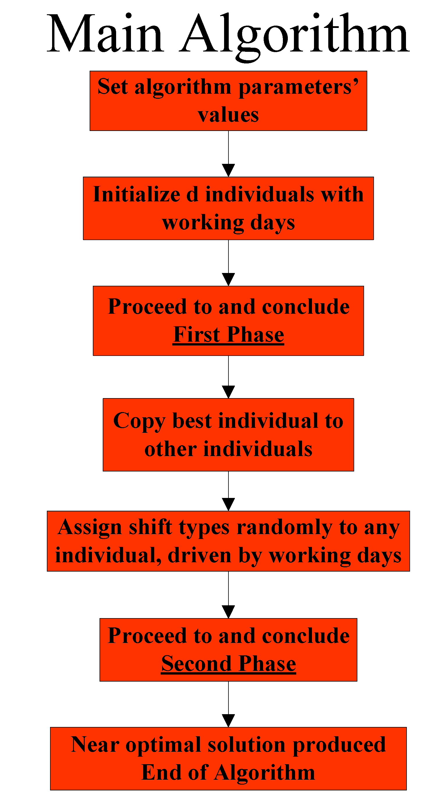
3.1. General Overview of the Stochastic Variable Neighborhood Algorithm

The flowchart describing the general overview of the proposed algorithm is presented in Figure 1. As shown there, the proposed algorithm is a hybrid one consisting of two phases:
(a)
The first phase deals with the assignment of nurses to working days
(b)
The second phase deals with the assignment of nurses to shift types
At first, the values of the algorithm’s parameters are set, namely, the population size, the maximum number of repetition cycles of first phase, the maximum number of generations of second phase and, finally, the swapping probability (see Subsection 3.2). Due to the differences in nature, structure, philosophy and type of hard and soft constraints among input instances, there is a small difference in the swapping probability value used for each instance. Note that the value of swapping probability determines the searching behavior of the algorithm. A high value will cause an exhausting cell swap, while a low value will cause skipping of cell swaps (see Subsection 3.2). Exhaustive experiments showed that for some instances, a lower value of the swapping probability is beneficial to the algorithm, while the opposite holds for others. Except for swapping probability, the values used for the other algorithm’s parameters are the same. Table 1 lists the parameters’ values for each instance, as well as the time consumed in order to find the optimal parameters of the algorithm. The effect of parameter setting to algorithm performance is investigated in Section 5.1.
Figure 1. The structure of the proposed stochastic variable neighborhood search algorithm.
Algorithms 06 00278 g001
Table 1. The parameters’ values used for each input instance.
NoInput instanceSwapping probability (pswap)Number of cycles in first phaseMaximum number of generations in second phasePopulation sizeNumber of experiments needed to find the optimal parameters of the algorithmAverage time per experimentAverage time consumed
1Valouxis-10.9999511002222 min44 min
2BCV3-46.20.97110022211 min242 min
3MUSA0.9711002220.06 s1.32 s
4LLR0.511002170.56 s9.52 s
5BCV4-13.10.9711002223 s66 s
6WHPP0.4511002177.7 s130.9 s
7HED010.85110022729 s13.05 min
The experimentation procedure in order to find the optimal parameters of the algorithm is described as follows. At first, the number of cycles in the first phase was determined. For each input instance, we ran five experiments setting the number of cycles equal to 1, 2, 3, 4 and 5, respectively. For all instances, experimental results showed that a number of cycles equal to 1 suffices in order to achieve the best possible results. Next, the population size was determined. For each input instance, we ran five experiments, setting the population size equal to 1 to 5, respectively. For all instances, experimental results showed that a population size equal to 2 achieves the best possible results. The maximum number of generations in the second phase was set arbitrarily equal to 100, which is a very big value, since our main purpose was to reach or even beat the best ever reported roster for each input instance. However, as mentioned in Section 3.3, the user is able to choose the termination criterion he/she likes to apply between the maximum number of generations and the number of generations for which the fitness remains the same; that is, no improvement is reported.
Finally, we determined the value of the swapping probability (pswap) that leads the algorithm to the best possible results. At first, for each input instance, we ran seven experiments, setting pswap equal to 0.4, 0.5, 0.6, 0.7, 0.8, 0.9 and 1.0. For the sixth instance, since pswap = 0.4 was the value giving the best results, we further experimented, setting pswap equal to 0.35, 0.36, 0.37, 0.38, 0.39, 0.41, 0.42, 0.43, 0.44 and 0.45. Since pswap = 0.45 was the value giving the best results, we further experimented, setting pswap equal to 0.445, 0.446, 0.447, 0.448, 0.449, 0.451, 0.452, 0.453, 0.454 and 0.455. Since again pswap = 0.45 was the value giving the best results, we decided to use this value. For the fourth instance, since pswap = 0.5 was the value giving the best results, we further experimented, setting pswap equal to 0.45, 0.46, 0.47, 0.48, 0.49, 0.51, 0.52, 0.53, 0.54 and 0.55. Since again pswap = 0.5 was the value giving the best results, we decided to use this value. For the seventh instance, since pswap = 0.8 was the value giving the best results, we further experimented, setting pswap equal to 0.75, 0.76, 0.77, 0.78, 0.79, 0.81, 0.82, 0.83, 0.84 and 0.85. Since pswap = 0.85 was the value giving the best results, we further experimented, setting pswap equal to 0.845, 0.846, 0.847, 0.848, 0.849, 0.851, 0.852, 0.853, 0.854 and 0.855. Since again pswap = 0.85 was the value giving the best results, we decided to use this value. For the second, the third and the fifth instances, since pswap = 1.0 was the value giving the best results, we further experimented, setting pswap equal to 0.95, 0.96, 0.97, 0.98 and 0.99. Since pswap = 0.97 was the value giving the best results, we further experimented, setting pswap equal to 0.965, 0.966, 0.967, 0.968, 0.969, 0.971, 0.972, 0.973, 0.974 and 0.975. Since again pswap = 0.97 was the value giving the best results, we decided to use this value for these two instances. For the rest instances, namely, the first instance, since initially pswap = 1.0 was the value giving the best results, we further experimented, setting pswap equal to 0.95, 0.96, 0.97, 0.98 and 0.99. Since again pswap = 1.0 was the value giving the best results, we further experimented, setting pswap equal to 0.995, 0.996, 0.997, 0.998 and 0.999. Since again pswap = 1.0 was the value giving the best results, we further experimented, setting pswap equal to 0.9995, 0.9996, 0.9997, 0.9998 and 0.9999. Although, once again pswap = 1.0 was the value giving the best results, we decided to use pswap = 0.99995, since a value of pswap = 1.0 would make the execution of swaps deterministic and not stochastic. Using pswap = 1.0 would lead the algorithm to poor diversification and big intensification. To conclude, we noticed that for all instances, setting pswap to a big value causes big intensification, while setting pswap to a small value causes big diversification.
After setting the parameters’ values, the initialization of each individual of the proposed algorithm’s population takes place. This is done at random with respect to the working requirements of each day. Next, the first phase of the algorithm, which deals with the assignment of nurses to working days, is executed. After the first phase is completed, the best individual found is copied to all individuals of the population, and shift types are randomly assigned to them. Therefore, the input to the second phase of the algorithm is a population of individuals, all of them being equivalent, by means of workings, to the best individual found by the first phase, with shift types randomly assigned to them. Finally, the second phase of the algorithm, which deals with the assignment of nurses to shift types, is executed, leading to the near optimal solution found by the proposed algorithm.
Since the seven nurse rostering input instances, to which the proposed algorithm is applied, are totally different cases of nurse rostering problems, there are significant differences, between them, in nature, structure, philosophy and type of hard and soft constraints. As a result, a different evaluation function is used for each different input instance taking into account different constraints and having different weight values. The specific constraints and the weight values used for each different constraint for each different input instance are the ones presented in [38]. However, a general form of the evaluation function applied to all instances can be presented as follows:
Weight_function(Weight_of_1st_Constraint) × Times_1st_Constraint_is_violated + … + Weight_function(Weight_of_nth_Constraint) × Times_ nth_Constraint_is_violated
where the ith Constraint is different for each different input instance, Weight_of_ith_Constraint is the weight of the ith Constraint (which is different for each different input instance) and Times_ith_Constraint_is_violated is the number of times the ith Constraint is violated. In addition, Weight_function(Weight_of_ith_Constraint) equals Weight_of_ith_Constraint, if the ith Constraint is assumed linear, while Weight_function(Weight_of_ith_Constraint) equals Weight_of_ith_Constraint × Weight_of_ith_Constraint if the ith Constraint is assumed quadratic. Whether a constraint is assumed linear or quadratic depends, once again, on the input instance, and it is explicitly stated. At this point, we have to mention that for all input instances, the evaluation function takes into account only constraints concerning working days and day offs in the first phase of the algorithm, while it takes into account all kinds of constraints in the second phase of the algorithm.

3.2. The First Phase of the Stochastic Variable Neighborhood Algorithm

The first phase of the proposed algorithm, which deals with the assignment of nurses to working days, is presented in Figure 2. As shown, this phase consists of the execution of procedure Successive_Segment_Swap_Mutation(). This procedure is applied to each individual sequentially and is repeated for a specified number of cycles. A detailed description of this procedure along with procedure Selective_Partial_Swap(), which is used by Successive_Segment_Swap_Mutation() in the first phase of the algorithm, is given in the following paragraphs.
Figure 2. The structure of the first phase of the proposed stochastic variable neighborhood search algorithm.
Algorithms 06 00278 g002
The procedure, Successive_Segment_Swap_Mutation(), is applied as follows. At first, a list of all nurses L1 is created at random. Next, for each nurse n1 in L1 and for each nurse, n2, next to n1 (i.e., after n1 in L1), procedure Selective_Partial_Swap() is applied. This procedure, which is described in the next paragraph, is applied between nurse n1 and other nurses, until no other nurse n2 exists in list L1 and is repeated from the beginning for each nurse, n1, in list, L1. The structure of Successive_Segment_Swap_Mutation() is presented in Figure 3.
Figure 3. The structure of the procedure, Successive_Segment_Swap_Mutation().
Algorithms 06 00278 g003
Procedure Selective_Partial_Swap(), which in fact implements a “stochastic moving segment grouping swap”, is applied for each day, d1, of the scheduling period as follows. At first, the left extreme (this is always equal to d1) and the right extreme (this is equal to d2) of the cell segment, in which swaps will be performed, are defined. Next, swaps are performed between cells included in a cell segment defined previously for rosters belonging to nurse n1 and nurse n2 under a certain probability. After all swaps in the selected cell segment have been performed, the fitness of the roster is computed. If the fitness of the created roster (i.e., after the swaps) is improved, then the swaps are accepted; otherwise, the swaps are discarded, and the roster sustains the structure it had before the swaps. After that, d2 is increased by one, and swapping cells between d1 and d2 for rosters belonging to nurses n1 and n2 is repeated as long as d2 is less or equal to the last day of the scheduling period. The structure of this procedure is presented in Figure 4. At this point, we have to mention that the application of a “stochastic moving segment grouping swap” to the nurse rostering problem is innovative, to our knowledge.
Figure 4. The structure of the procedure, Selective_Partial_Swap().
Algorithms 06 00278 g004

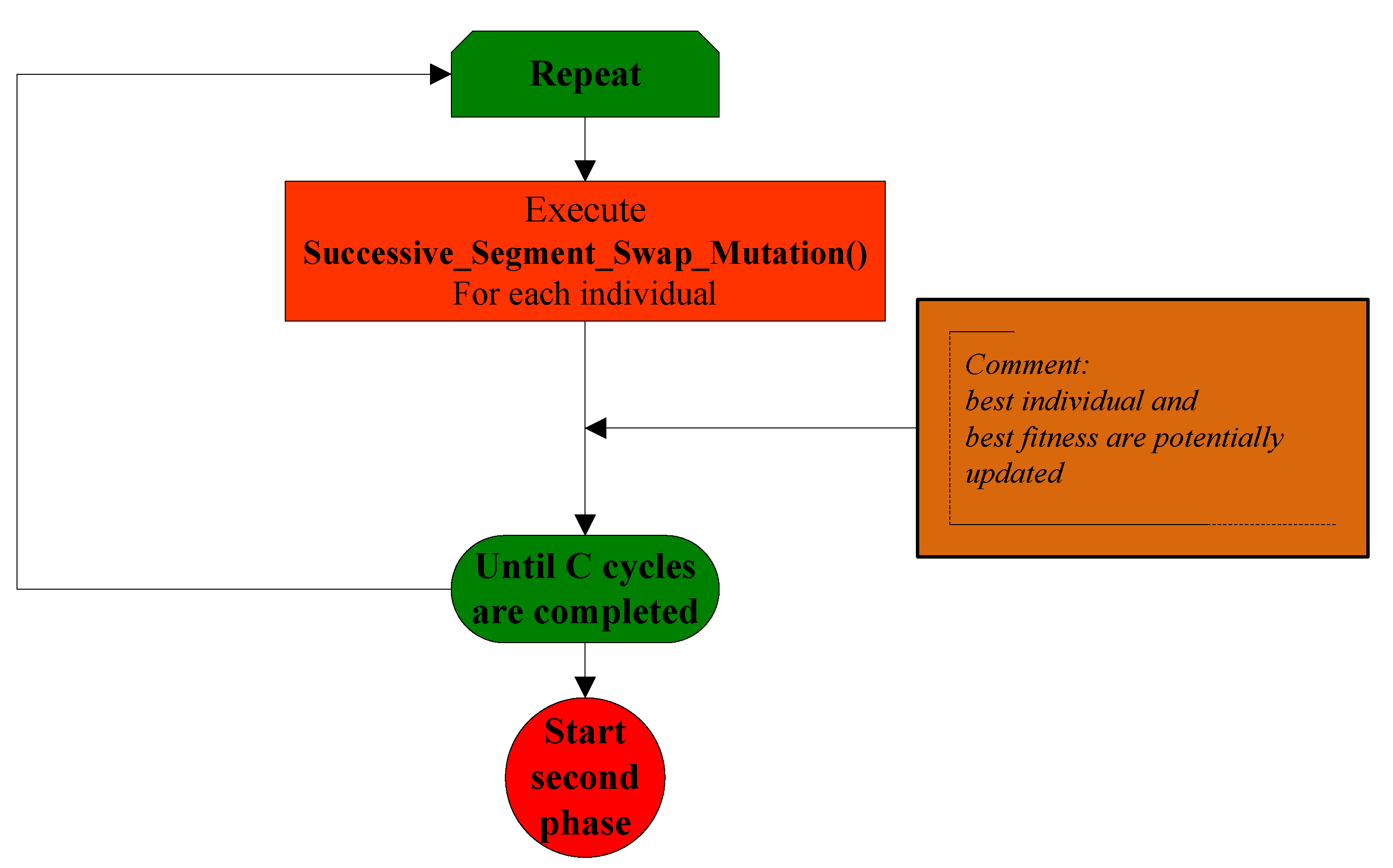
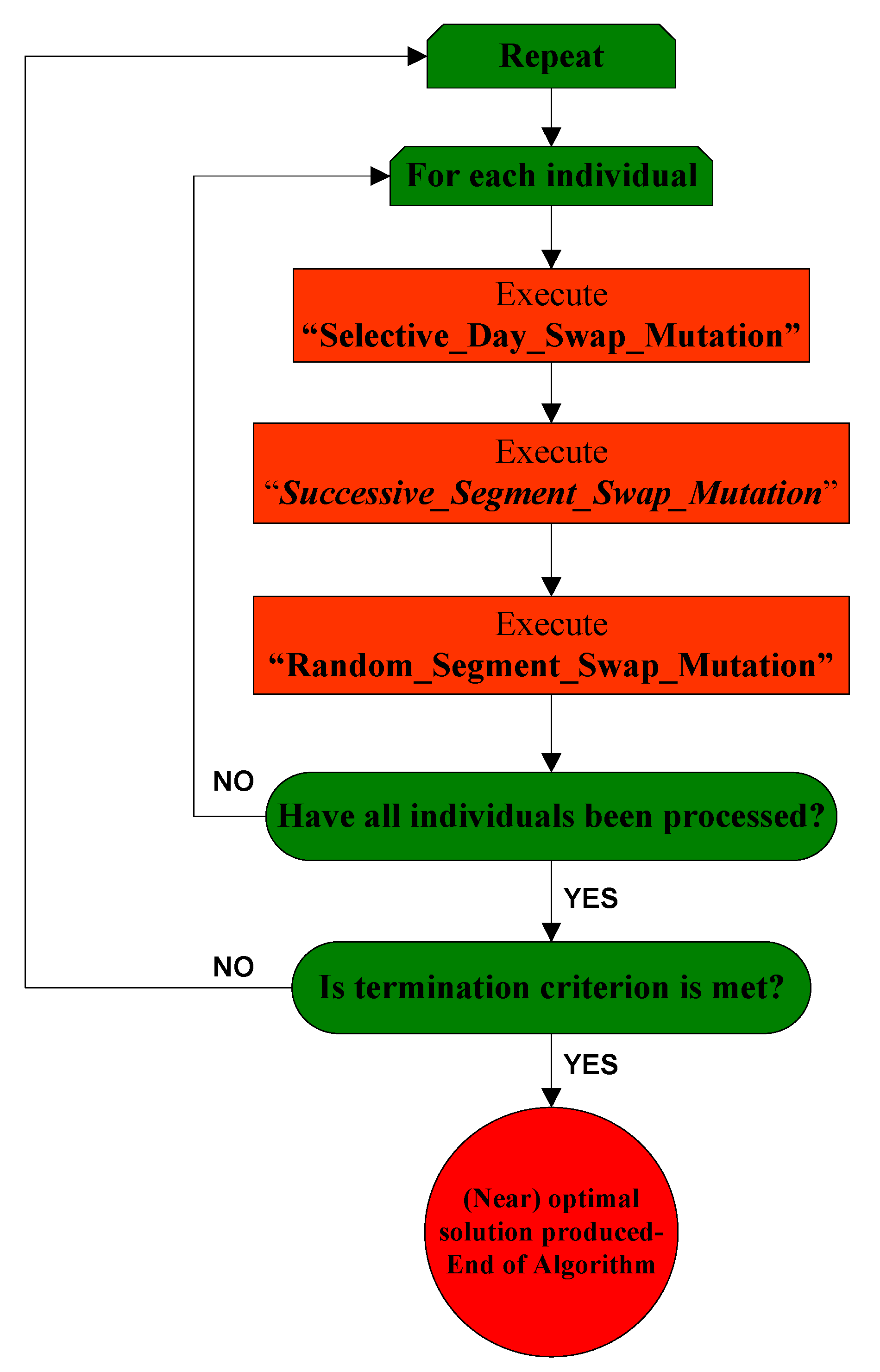
3.3. The Second Phase of the Algorithm

The second phase of the proposed algorithm, which deals with the assignment of nurses to shift types, is presented in Figure 5. As shown, this phase consists of the sequential execution of the following procedures:
(a) 
Selective_Day_Swap_Mutation()
(b) 
Successive_Segment_Swap_Mutation()
(c) 
Random_Segment_Swap_Mutation()
Procedure Successive_Segment_Swap_Mutation() is the same with the one executed in the first phase of the algorithm; however, this time, it is executed in order to assign nurses to shift types and not to working days as performed in the first phase. This is the goal of the other two procedures, too. The execution of these three procedures is repeated for each individual of the population for a number of times, i.e., generations. The execution of the second phase of the algorithm is performed, until a specified termination criterion is met. We have implemented two termination criteria, which are the following:
The total number of generations
The number of generations for which the fitness remains the same, that is, no improvement is reported
Figure 5. The structure of the second phase of the proposed stochastic variable neighborhood search algorithm.
Algorithms 06 00278 g005
More precisely, at the beginning of the algorithm, the user is asked to select the termination criterion he/she prefers to use:
  • If he/she chooses “the total number of generations”, next, he/she has to insert this number.
  • If he/she chooses “the total number of generations for which the fitness remains the same”, next, he/she has to insert this number.
In the next sections, we present a detailed description of procedures, Selective_Day_Swap_Mutation() and Random_Segment_Swap_Mutation().

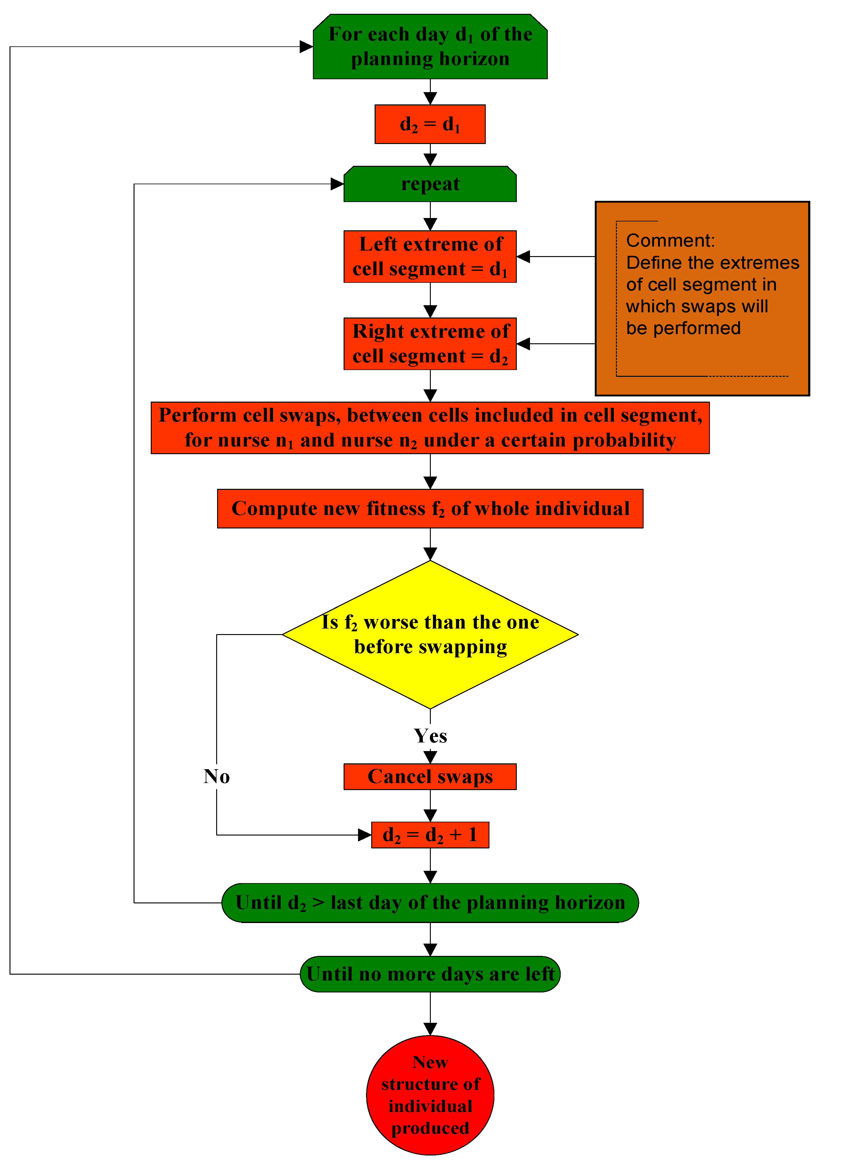
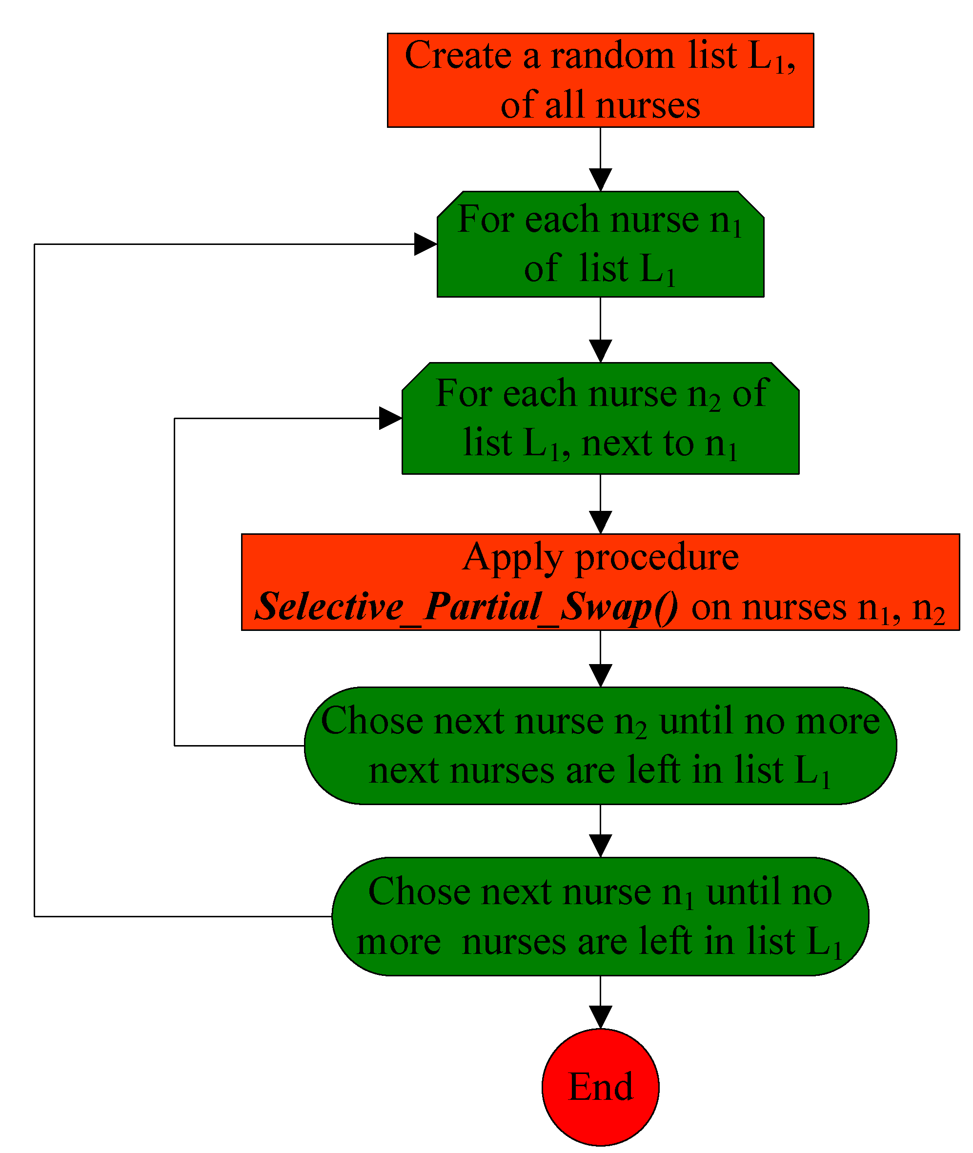
3.3.1. Procedure Selective_Day_Swap_Mutation()

This procedure is applied as follows. At first, a nurse, n1, is selected at random. Next, the order of all combinations between nurse n1 and all other nurses is created randomly. Then, for each day of the scheduling period and for each pair of nurses created at random, a swap is performed between the cells of the current day of each pair of nurses. If the fitness of the created roster (i.e., after the swap) is improved, then the swap is accepted; otherwise, the swap is discarded, and the roster sustains the structure it had before the swap. This procedure is performed for each nurse of the roster. The structure of this procedure is presented in Figure 6.
Figure 6. The structure of the procedure, Selective_Day_Swap_Mutation().
Algorithms 06 00278 g006

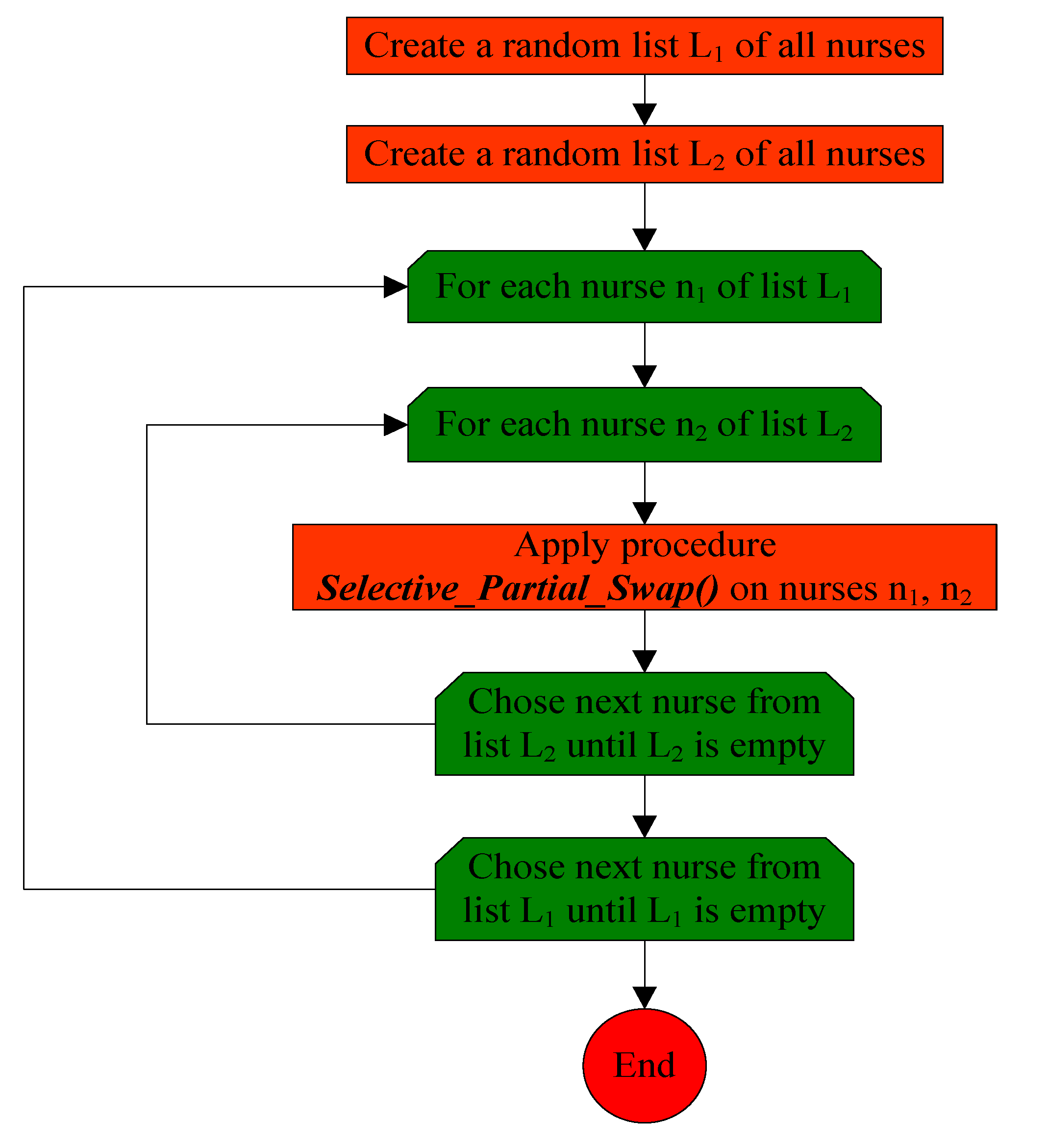
3.3.2. Procedure Random_Segment_Swap_Mutation()

This procedure is applied as follows. At first, a list of all nurses in random order, L1, and a list of all nurses in a random order, too, L2, are created. Next, for each nurse, n1, in list L1 and for each nurse, n2, in list L2, procedure Selective_Partial_Swap() is applied. This procedure, which is described in the previous section, is applied between nurse n1 and each nurse, n2, belonging to list, L2, until no other nurse n2 exists in list L2 and is repeated from the beginning for each nurse n1 in list L1. The structure of this procedure is presented in Figure 7.
Figure 7. The structure of the procedure, Random_Segment_Swap_Mutation().
Algorithms 06 00278 g007

4. Input Data

As stated in the Introduction Section, the proposed two-phase variable neighborhood algorithm is applied to seven different nurse rostering input instances. These instances, which have significant differences with each other, are presented in the following sections. They comprise a set of benchmark data that represents a wide variety of nurse rostering problems with non-trivial properties, which are derived from complete real world complex instances.

4.1. Input Instance, Valouxis-1

In this input instance, there are 16 nurses working three daily work shift types, and the planning horizon is 28 days long. The demand is assumed to be the same every week, and the daily requirement for personnel from Monday to Friday is 4-4-2 for the Day, Evening and Night work shifts, respectively, and the demand for Saturday and Sunday is 3-3-2, respectively. The legal work stretches are 2–4 days long, while the least time break between two work stretches is two calendar days long. In the planning horizon, all individuals must have at least one Sunday rest, while the total Day, Evening and Night work shifts must be 5–8, 5–8 and 2–5, respectively. The total work shifts of all types must be 15–18 work shifts. A specific description of the precise definition of the evaluation function used, the hard and soft constraints and their respective weight values is given in [39]. For a more detailed description of this input instance, the reader can refer to [32].

4.2. Input Instance, BCV3-46.2

This input instance was collected from a rather small department of a real hospital, using the nurse rostering model and algorithms developed at KaHo Sint-Lieven [40]. It comprises a non-cyclic problem. The number of nurses equals 46, the number of shift types equals 3 (Day, Early, Late and Night), the scheduling period is 26 days long and there is only one skill level (Nurse). A specific description of the precise definition of the evaluation function used, the hard and soft constraints and their respective weight values is given in [41]. For a more detailed description of this input instance, the reader can refer to [34].

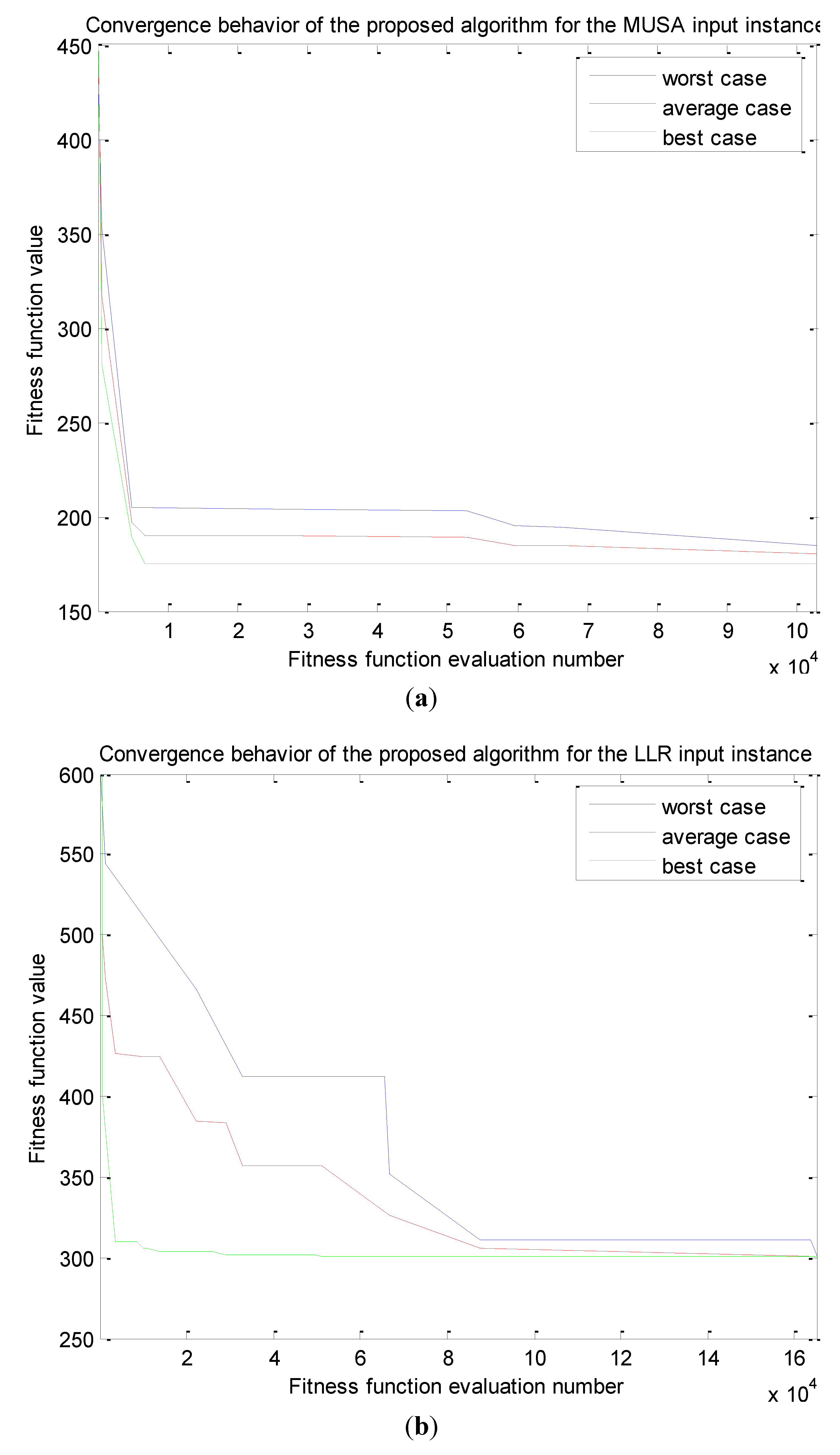
4.3. Input Instance, MUSA

In this input instance, there are 11 nurses, there is only one shift type (Day), the scheduling period is 14 days long and there is only one skill level (Nurse). A specific description of the precise definition of the evaluation function used, the hard and soft constraints and their respective weight values is given in [42]. For a more detailed description of this input instance, the reader can refer to [36].

4.4. Input Instance, LLR

This input instance belongs to a class of over-constrained nurse rostering problems. The number of nurses equals 27, the number of shift types equals 3 (Morning, Afternoon and Night), the scheduling period is seven days long and there is only one skill level (Nurse). A specific description of the precise definition of the evaluation function used, the hard and soft constraints and their respective weight values is given in [43]. For a more detailed description of this input instance, the reader can refer to [33].

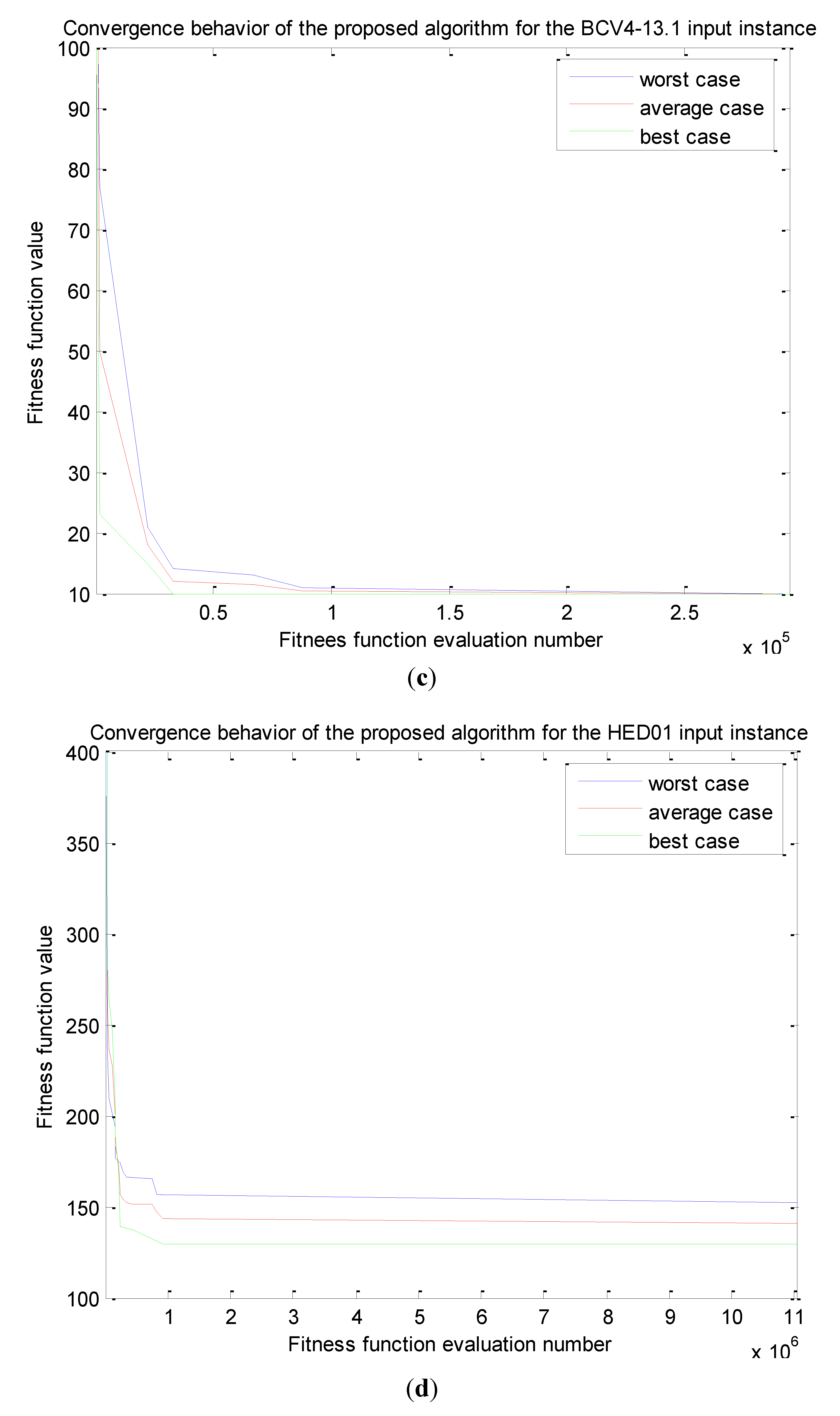
4.5. Input Instance, BCV4-13.1

This input instance was also collected from a rather small department at a real hospital, using the nurse rostering model and algorithms developed at KaHo Sint-Lieven [40]. It comprises a non-cyclic problem. The number of nurses equals 13, the number of shift types equals 4 (Day, Early, Late and Night), the scheduling period is 29 days long and there are two skill levels (Nurse and Head nurse). A specific description of the precise definition of the evaluation function used, the hard and soft constraints and their respective weight values is given in [44]. For a more detailed description of this input instance, the reader can refer to [34].

4.6. Input Instance, WHPP

In this instance, the number of nurses equals 30, the number of shift types equals 3 (Day, Early and Night), the scheduling period is 14 days long and there is only one skill level (Nurse). A specific description of the precise definition of the evaluation function used, the hard and soft constraints and their respective weight values is given in [45]. For a more detailed description of this input instance, the reader can refer to [37].

4.7. Input Instance, HED01

This input instance stems form the needs of an actual hospital emergency department (HED) in Spain. An actual situation set up by the HED’s management is described. HED’s permanent staff consists of 16 workers, while there are also four temporary workers. The number of shift types equals 5 (Weekday morning—M; Weekday afternoonA; Weekday night—N; Weekday stand-by duty—D; and Holiday stand-by duty—H), the scheduling period is 31 days long and there are two skill levels (Permanent staff and Temporary staff). Moreover, a minimum number of doctors must be assigned to each working shift. As a general rule for working days, different members of staff will be assigned to the different existing shifts: Four members will be assigned to the morning (M) and afternoon (A) shifts; two will be assigned to the night (N) shift; and one person will be on 24 h weekday stand-by duty (D). On Saturdays, Sundays and holidays, the HED’s medical staff will work on duty, whereby four members of staff will generally work for an uninterrupted 24 h holiday stand-by duty (H). A specific description of the precise definition of the evaluation function used, the hard and soft constraints and their respective weight values is given in [46]. For a more detailed description of this input instance, the reader can refer to [35].

5. Computational Results

The proposed two-phase stochastic variable neighborhood search algorithm approach is coded in C++ and is run on Intel® Core™ 2 Duo CPU E7500 2.93 GHz under the Windows 7 OS. The algorithm parameters’ values used are the ones presented in Table 1, Section 3.1. In order to demonstrate its efficiency and very good performance, the proposed algorithm is compared with six very effective algorithms for solving the nurse rostering problem issued in the literature [32,33,34,35,36,37] in solving the same seven input instances.
In Table 2, the performance and efficiency of the proposed two-phase stochastic variable neighborhood search algorithm is shown by comparing the best timetables constructed by it with the best timetables created by the other six algorithms for each different input instance. Since in [32,33,34,35,36,37] the best rosters created are presented, we also decided in the current contribution to present and compare the best rosters constructed by the proposed approach in order to have a fair comparison between the algorithms. Note that, for each different input instance, in order to compare the roster constructed by the proposed variable neighborhood search algorithm and the roster constructed by the respective published nurse rostering algorithm, we used the same fitness function, the same hard and soft constraints and the same constraint weights as the ones used by the respective algorithms.
Table 2. Comparing the best timetables constructed by the proposed algorithm with the best timetables created in [32,33,34,35,36,37].
Input instancePublished algorithmProposed algorithm
Description of algorithmFitness valueExecution timeFitness valueExecution time
Valouxis-1Integer linear programming approach [32]16015 min2017.64 s
BCV3-46.2A shift sequence based approach with greedy local search and adaptive ordering [34]36013 min, 4 s89416 min
MUSASingle phase goal programming model [36]19928.3 s1750.12 s
LLRTwo-phase hybrid approach [33]5101 min, 36 s3010.3 s
BCV4-13.1A shift sequence based approach with greedy local search without adaptive ordering [34]1810 s103 s
WHPPLinear programming formulation using column generation approach [37]5Not mentioned59.1 s
HED01Genetic algorithm [35]517Not mentioned12929.1 s
Table 2 demonstrates that the proposed algorithm outperforms other published approaches in 6/7 cases (85.7%), considering the best roster per instance, while it achieves the same result in 1/7 cases (14.3%). From experimental results presented in Table 2, one can easily come to the conclusion that the proposed algorithm is very efficient and achieves better results compared to the other six techniques issued in the literature that have been applied to the same instances of the nurse rostering problem.
Moreover, in order to demonstrate the efficiency and very satisfactory performance of the proposed two-phase variable neighborhood search algorithm, the best rosters found by it are compared with the best-known timetables ever reported for the same seven different input nurse rostering instances [38].
Table 3 demonstrates that the proposed two-phase algorithm manages to reach the best known fitness ever reported in the literature in 6/7 cases (85.7%), while it manages to beat the best known fitness ever reported in the literature in 1/7 cases (14.3%). From experimental results presented in Table 3, one can easily come to the conclusion that the proposed algorithm is very efficient and achieves results equal to the best known ever reported for the majority of these quite different nurse rostering instances, while it manages to beat the best known ever reported result in one case. Except for that, the proposed algorithm has demonstrated experimentally that the best result ever reported for these six instances is not unique, since the best nurse rosters that the proposed algorithm created are in all six cases different from the best ones ever reported [38]. This means that in these six cases, there are at least two different best ever reported rosters and that maybe the global optimum is yet to be found. The executables implementing the proposed stochastic variable neighborhood search algorithm, as well as the best rosters achieved for each input instance, can be accessed in [47].
Table 3. Comparing the best timetables constructed by the proposed algorithm with the best timetables ever reported for these specific instances.
Input InstanceBest roster reported ever [38]Best roster found by the proposed algorithm
Found byFitness valueExecution TimeFitness valueExecution Time
Valouxis-1Tim Curtois, 3/9/200820Not mentioned2017.64 s
BCV3-46.2F. Xue, C. Y. Chan and W. H. Ip, using a Hybrid VDS, 2/8/20088944 h, 57 min89416 min
MUSANot mentioned175Not mentioned1750.12 s
LLRTim Curtois, using a variable depth search, 5/9/200830110 s3010.3 s
BCV4-13.1Not mentioned10Not mentioned103 s
WHPPWeil et al., 5/4/20095Not mentioned59.1 s
HED01Tec on BEECHBONE (CS), 11/2/2010136Not mentioned12929.1 s
The superiority of the proposed algorithm compared to other approaches comes mainly from the fact that the algorithm succeeds in searching the search space using a new variable neighborhood search approach. In the literature, there are three commonly used swaps, that is, simple move, simple swap and Kempe swap, each one of them leading to a search algorithm to investigate a different neighborhood [23]. The proposed algorithm uses only simple swaps, that is, swaps between cells without considering what these cells contain in order to perform the swap (i.e., whether they are empty or not). However, each one of the three swap procedures used by the proposed algorithm (see Section 3.2, Section 3.3.1 and Section 3.3.2) applies a different swap mechanism, which leads the algorithm to search in a different neighborhood of the search space. The application of the proposed mutation operators that implement the algorithm’s swapping mechanisms, applied in this specific way and order, is innovative to our knowledge and different from the swapping mechanisms already investigated in [13].The strongest point of this variable neighborhood search approach is the combination of a classic neighborhood search with a “stochastic moving segment grouping swap” (see Subsection 3.2). The “stochastic moving segment grouping swap” achieves exhaustive local search, since the segment is not stable, and as a result, it ensures intensification. On the other hand, since this swap is a stochastic one, it ensures diversification. To conclude, combining and applying these three swap procedures (see Section 3.2, Section 3.3.1 and Section 3.3.2) enriches the variable neighborhood search approach, since it enhances the classic neighborhood search with a “stochastic moving segment grouping swap”. This combination ensures both intensification and diversification of the search space.
Since the nature of the proposed two-phase algorithm is stochastic, different computational results may be obtained in different runs. So, in order to demonstrate its efficiency, in Table 4, we present not only the best, but also the worst and the average results (and the respective standard deviations—STDs), considering the fitness function value achieved and the execution time of the algorithm. Additionally, we present the respective coefficient of variation (CV) and the success rate for each input instance. All results presented in Table 4 concern the execution of the proposed algorithm to the seven aforementioned nurse rostering input instances for 100 Monte Carlo runs.
Table 4. Computational experiments demonstrating the efficiency, stability and homogeneity of the proposed algorithm. STD, standard deviation; CV, coefficient of variation.
Input instanceFitness valueExecution TimeSuccess Rate
BestWorstAverageSTDCV (%)BestWorstAverageSTD
Valouxis-12012073.3330.5541.717.64 s222.88 s90.19 s75.620%
BCV3-46.28948948940016 min31 min25 min4.37100%
MUSA175175175000.12 s0.52 s0.22 s0.13100%
LLR301305301.480.930.30.3 s5.5 s1.85 s1.467%
BCV4-13.1101010003 s14.2 s7.1 s0.7100%
WHPP555009.1 s27.2 s16.2 s5.9100%
HED01129156143.287.885.529.1 s5 min, 40 s2 min, 47 s2.136%
Experimental results presented in Table 4 show that the average fitness reached by the proposed two-phase variable neighborhood search approach is, in most cases, very close to the best one achieved for each input instance. This demonstrates that the proposed algorithm is stable and efficient. We also notice that CV of fitness function value ranges from 0% to 41.7%, with the great majority of CV values being below 10%. More specifically, in four out of seven cases, CV equals 0, which means that the algorithm is totally homogenous. This observation leads to the conclusion that the behavior of the algorithm concerning the resulted fitness function value for 100 Monte Carlo runs per input instance is quite homogenous. Note that we have intentionally avoided calculating CV values for the execution time. This is done because STD and average values are close to each other, so the CV value for the execution time would be misleading. Moreover, in Table 4, we present the success rate, i.e., the percentage of cases that the proposed algorithm achieves the best fitness function value among 100 Monte Carlo runs. The fact that, in most cases, the success rate achieved is bigger than 60%, demonstrates the efficiency of the proposed algorithm. In addition, in four cases, the success rate is 100%.
Finally, we present convergence results (maximum, average and minimum evaluation function value versus number of function evaluations) in order to illustrate the evolutionary behavior of the proposed algorithm. Figure 8 illustrates the convergence behavior of the proposed algorithm for four input instances, namely, MUSA, LLR, BCV4-13.1 and HED01. In all cases, the algorithm’s convergence behavior is very satisfactory, since it avoids falling into local optima very quickly and shows significant improvement during the evolutionary process. In these experiments, because our main concern was to reach or even beat the best ever reported result for each different input instance, we used as the determination criterion “the total number of generations”.
Figure 8. Convergence behavior of the proposed algorithm for four input instances: (a) Input instance, MUSA; (b) Input instance, LLR; (c) Input instance, BCV4-13.1; (d) Input instance HED01.
Algorithms 06 00278 g008aAlgorithms 06 00278 g008b

Investigating the Effect of Parameter Setting to Algorithms’ Performance

In this section, the effect of parameter setting to algorithms’ performance is investigated and the results of different specific parameter values are demonstrated. Except for that, an indication of the contribution of each component of the algorithm is presented. More specifically, the contribution of the two-phase approach compared to a single-phase approach is investigated. As stated in Section 3.1, the first phase of the algorithm deals with the assignment of nurses to working days, while the second phase of the algorithm deals with the assignment of nurses to shift types. Therefore, the first phase of the algorithm cannot solve the nurse rostering problem alone, while the second phase can be applied to solve the nurse rostering problem as a single-phase approach. Experimental results presented below, show that using together the first and the second phase of the algorithm, as a two-phase approach, achieves better results to using only the second phase of the algorithm as a single-phase approach.
Due to the fact that there are no obvious criteria for defining specific parameter values of the proposed algorithm for all instances of the problem, we have selected these values by trial and error. More precisely, we have conducted exhaustive experiments and selected the values that achieved the best simulation results and the best algorithm’s behavior. Table 5, Table 6, Table 7, Table 8, Table 9, Table 10, Table 11, Table 12, Table 13, Table 14, Table 15, Table 16, Table 17, Table 18, Table 19, Table 20, Table 21, Table 22, Table 23, Table 24 and Table 25 presented in the next paragraphs, show the effect of the value of first phase’s number of cycles, the effect of the value of the population size and the effect of the value of swapping probability to algorithms’ performance and behavior.
In Table 5, Table 6 and Table 7, experimental results that investigate the effect of parameter setting to algorithms’ performance and behavior regarding input instance Valouxis-1 are presented.
As shown in Table 5, setting the first phase’s number of cycles equal to 1 assists the algorithm in achieving the lowest best and average fitness values in the lowest best and average execution times, respectively. Except for that, if we do not use the first phase at all (first phase cycles = 0), experimental results are rather worse.
Table 5. Investigating the effect of first phase’s number of cycles for input instance, Valouxis-1.
Input instance Valouxis-1Fitness valueExecution time (s)Success rate
BestWorstAverageSTDCV (%)BestWorstAverageSTD
First phase cycles = 0401608834.2538.928017011024.610%
First phase cycles = 12012073.3330.5541.717.64222.8890.1975.620%
First phase cycles = 2401408335.9243.278518010031.820%
First phase cycles = 3401608634.0639.69018015027.610%
First phase cycles = 4401406828.642.0511021018043.820%
First phase cycles = 5401206821.531.627829023234.0810%
As shown in Table 6, setting the value of population size equal to 2 assists the algorithm in achieving the lowest best and average fitness values in the lowest best and average execution times, respectively.
Table 6. Investigating the effect of population size for input instance, Valouxis-1.
Input instance Valouxis-1Fitness valueExecution time (s)Success rate
BestWorstAverageSTDCV (%)BestWorstAverageSTD
POPSIZE = 1601408830.1134.21611801303630%
POPSIZE = 22012073.3330.5541.717.64222.8890.1975.620%
POPSIZE = 3601608334.0140.976224613557.330%
POPSIZE = 46014010028.2828.2872222.91405510%
POPSIZE = 5601008420.6624.59802001506230%
As shown in Table 7, setting the value of swapping probability equal to 0.99995 assists the algorithm in achieving both the lowest best fitness value and the highest success rate.
Table 7. Investigating the effect of swapping probability for input instance, Valouxis-1.
Input instance Valouxis-1Fitness valueExecution time (s)Success rate
BestWorstAverageSTDCV (%)BestWorstAverageSTD
Swapping probability = 0.85401208225.7331.371001901503310%
Swapping probability = 0.9201607640.8853.788020011238.410%
Swapping probability = 0.95401006819.3228.416625312960.920%
Swapping probability = 0.97201006024.9441.561893.67139.2410%
Swapping probability = 0.999952012073.3330.5541.717.64222.8890.1975.620%
In Table 8, Table 9 and Table 10, experimental results that investigate the effect of parameter setting to algorithms’ performance and behavior regarding input instance BCV3-46.2 are presented.
As shown in Table 8, setting the first phase’s number of cycles equal to 1 assists the algorithm in achieving the lowest best and average fitness values in the lowest best and average execution times, respectively. Except for that, if we do not use the first phase at all (first phase cycles = 0), execution times are rather worse.
Table 8. Investigating the effect of first phase’s number of cycles for input instance, BCV3-46.2.
Input instance BCV3-46.2Fitness valueExecution time (min)Success rate
BestWorstAverageSTDCV (%)BestWorstAverageSTD
First phase cycles = 0894894894002542315.55100%
First phase cycles = 1894894894001631254.37100%
First phase cycles = 28948948940021453911.52100%
First phase cycles = 38948948940019573511.94100%
First phase cycles = 4894894894002649386.13100%
First phase cycles = 5894894894003049405.6100%
As shown in Table 9, setting the value of population size equal to 2 assists the algorithm in achieving the lowest best and average fitness values in the lowest best and average execution times, respectively.
Table 9. Investigating the effect of population size for input instance, BCV3-46.2.
Input instance BCV3-46.2Fitness valueExecution time (min)Success rate
BestWorstAverageSTDCV (%)BestWorstAverageSTD
POPSIZE = 1894894894001648288.71100%
POPSIZE = 2894894894001631254.37100%
POPSIZE = 3894894894001638287.64100%
POPSIZE = 4894894894001743348100%
POPSIZE = 5894894894002542335.55100%
As shown in Table 10, setting the value of swapping probability equal to 0.97 assists the algorithm in achieving the lowest best fitness value in the lowest execution time.
Table 10. Investigating the effect of swapping probability for input instance, BCV3-46.2.
Input instance BCV3-46.2Fitness valueExecution time (min)Success rate
BestWorstAverageSTDCV (%)BestWorstAverageSTD
Swapping probability = 0.858948948940016573611.67100%
Swapping probability = 0.9894894894002349359.04100%
Swapping probability = 0.95894894894002751398.46100%
Swapping probability = 0.97894894894001631254.37100%
Swapping probability = 0.999958948948940011613012.84100%
In Table 11, Table 12 and Table 13, experimental results that investigate the effect of parameter setting to the algorithms’ performance and behavior regarding input instance, MUSA, are presented.
As shown in Table 11, setting the first phase’s number of cycles equal to 1 assists the algorithm in achieving the lowest best and average fitness values in the lowest best and average execution times, respectively. Except for that, if we do not use the first phase at all (first phase cycles = 0), execution times and success rate are rather worse.
Table 11. Investigating the effect of first phase’s number of cycles for input instance, MUSA.
Input instance MusaFitness valueExecution time (s)Success rate
BestWorstAverageSTDCV (%)BestWorstAverageSTD
First phase cycles = 0175185177.84.252.40.130.520.30.1275%
First phase cycles = 1175175175000.120.520.220.13100%
First phase cycles = 2175180175.73.92.20.330.580.430.1280%
First phase cycles = 3175180175.53.520.40.570.480.0785%
First phase cycles = 4175180177.64.22.40.390.620.540.1190%
First phase cycles = 5175180177.53.41.90.540.870.70.1490%
As shown in Table 12, setting the value of population size equal to 2 assists the algorithm in achieving the lowest best and average fitness values in the lowest best and average execution times, respectively.
Table 12. Investigating the effect of population size for input instance, MUSA.
Input instance MUSAFitness valueExecution time (s)Success rate
BestWorstAverageSTDCV (%)BestWorstAverageSTD
POPSIZE = 1175180175.651.10.620.310.540.40.0795%
POPSIZE = 2175175175000.120.520.220.13100%
POPSIZE = 3175175175000.510.740.60.12100%
POPSIZE = 4175175175000.190.820.50.24100%
POPSIZE = 5175175175000.430.750.580.11100%
As shown in Table 13, setting the value of swapping probability equal to 0.97 assists the algorithm in achieving the lowest best and average fitness value and the highest success rate.
Table 13. Investigating the effect of swapping probability for input instance, MUSA.
Input instance MUSAFitness valueExecution time (s)Success rate
BestWorstAverageSTDCV (%)BestWorstAverageSTD
Swapping probability = 0.85175185176.53.381.90.140.420.320.1480%
Swapping probability = 0.9175185176.53.381.90.120.380.20.180%
Swapping probability = 0.951751851763.161.790.110.290.180.0790%
Swapping probability = 0.97175175175000.120.520.220.13100%
Swapping probability = 0.99995175185177.623.7520.060.560.230.1462%
In Table 14, Table 15 and Table 16, experimental results that investigate the effect of parameter setting to algorithms’ performance and behavior regarding input instance, LLR, are presented.
As shown in Table 14, setting the first phase’s number of cycles equal to 1 assists the algorithm in achieving the lowest best and average fitness values and the highest success rate. Except for that, if we do not use the first phase at all (first phase cycles = 0), execution times and success rate are rather worse.
Table 14. Investigating the effect of first phase’s number of cycles for input instance, LLR.
Input instance LLRFitness valueExecution time (s)Success rate
BestWorstAverageSTDCV (%)BestWorstAverageSTD
1ST Phase cycles = 0301303301.70.820.270.82.521.150%
1ST Phase cycles = 1301305301.480.930.30.35.51.851.467%
1ST Phase cycles = 2301303301.80.80.312.91.60.645%
1ST Phase cycles = 3301303301.60.80.261.33.82.40.858%
1ST Phase cycles = 4301303301.40.70.231.33.42.80.762%
1ST Phase cycles = 5301303301.50.70.231.44.62.91.147%
As shown in Table 15, setting the value of population size equal to 2 assists the algorithm to achieve the lowest best and average fitness values and the highest success rate.
Table 15. Investigating the effect of population size for input instance, LLR.
Input instance LLRFitness valueExecution time (s)Success rate
BestWorstAverageSTDCV (%)BestWorstAverageSTD
POPSIZE = 1301305302.21.60.530.742.381.50.650%
POPSIZE = 2301305301.480.930.30.35.51.851.467%
POPSIZE = 3301303301.71.060.350.987.082.92.260%
POPSIZE = 4301303301.80.80.270.233.211.320.945%
POPSIZE = 5301303301.60.70.230.384.031.721.255%
As shown in Table 16, setting the value of swapping probability equal to 0.5 assists the algorithm in achieving the lowest best and average fitness values in the lowest best and average execution times, respectively, as well as the highest success rate.
Table 16. Investigating the effect of swapping probability for input instance, LLR.
Input instance LLRFitness valueExecution time (s)Success rate
BestWorstAverageSTDCV (%)BestWorstAverageSTD
Swapping probability = 0.4301303301.60.90.290.855.232.10.3355%
Swapping probability = 0.45301303301.50.550.181.275.662.21.3663%
Swapping probability = 0.5301305301.480.930.30.35.51.851.467%
Swapping probability = 0.55301303301.50.40.131.22.62.41.665%
Swapping probability = 0.6301303301.50.70.231.14.92.21.164%
In Table 17, Table 18 and Table 19, experimental results that investigate the effect of parameter setting to algorithms’ performance and behavior regarding input instance, BCV4-13.1, are presented.
As shown in Table 17, setting the first phase’s number of cycles equal to 1 assists the algorithm in achieving the lowest best and average fitness values in the lowest best and average execution times. For this specific input instance, if we do not use the first phase at all (first phase cycles = 0), experimental results are much less the same.
Table 17. Investigating the effect of first phase’s number of cycles for input instance, BCV4-13.1.
Input instance BCV4-13.1Fitness valueExecution time (s)Success rate
BestWorstAverageSTDCV (%)BestWorstAverageSTD
First phase cycles = 0101010005.847.236.210.52100%
First phase cycles = 110101000314.27.12.65100%
First phase cycles = 2101010006.9512.38.431.66100%
First phase cycles = 3101010007.4614.410.361.99100%
First phase cycles = 4101010009.4214.310.991.45100%
First phase cycles = 5101010009.351513.151.77100%
As shown in Table 18, setting the value of population size equal to 2 assists the algorithm in achieving the lowest best and average fitness values in the lowest best and average execution times, respectively.
Table 18. Investigating the effect of population size for input instance, BCV4-13.1.
Input instance BCV4-13.1Fitness valueExecution time (s)Success rate
BestWorstAverageSTDCV (%)BestWorstAverageSTD
POPSIZE = 1101010005.38.56.982.1100%
POPSIZE = 210101000314.27.12.65100%
POPSIZE = 3101010006.287.230.64100%
POPSIZE = 41010100068.36.950.9100%
POPSIZE = 5101010006.49.87.81.31100%
As shown in Table 19, setting the value of swapping probability equal to 0.97 assists the algorithm to achieve the lowest best and average fitness values in the lowest best and average execution times, respectively.
Table 19. Investigating the effect of swapping probability for input instance, BCV4-13.1.
Input instance BCV4-13.1Fitness valueExecution time (s)Success rate
BestWorstAverageSTDCV (%)BestWorstAverageSTD
Swapping probability = 0.85101010005.727.87.30.51100%
Swapping probability = 0.9101010005.237.557.30.61100%
Swapping probability = 0.95101010005.147.457.20.69100%
Swapping probability = 0.9710101000314.27.10.7100%
Swapping probability = 0.99995101010003.8722.112.456.61100%
In Table 20, Table 21 and Table 22, experimental results that investigate the effect of parameter setting to algorithms’ performance and behavior regarding input instance, WHPP, are presented.
As shown in Table 20, setting the first phase’s number of cycles equal to 1 assists the algorithm in achieving the lowest best and average fitness values in the lowest best and average execution times. Except for that, if we do not use the first phase at all (first phase cycles = 0), execution times and success rate are rather worse.
Table 20. Investigating the effect of first phase’s number of cycles for input instance, WHPP.
Input instance WHPPFitness valueExecution time (s)Success Rate
BestWorstAverageSTDCV (%)BestWorstAverageSTD
First phase cycles = 0575.20.6312.116.4597.4343.321.890%
First phase cycles = 1555009.127.216.25.9100%
First phase cycles = 2585.30.9517.925.7442.4375.490%
First phase cycles = 35550023.4351.633.89.35100%
First phase cycles = 45550025.1939.934.35.6100%
First phase cycles = 5555002154.3389.7100%
As shown in Table 21, setting the value of population size equal to 2 assists the algorithm in achieving the lowest best and average fitness values in the lowest best and average execution times, respectively.
Table 21. Investigating the effect of population size for input instance, WHPP.
Input instance WHPPFitness valueExecution time (s)Success rate
BestWorstAverageSTDCV (%)BestWorstAverageSTD
POPSIZE = 1585.30.9517.99.978.234.520.8490%
POPSIZE = 2555009.127.216.25.9100%
POPSIZE = 3575.20.6312.1212.458.13116.890%
POPSIZE = 4585.30.9517.919.251.333.610.7190%
POPSIZE = 55550018.589.837.621.9100%
As shown in Table 22, setting the value of swapping probability equal to 0.45 assists the algorithm in achieving the lowest best and average fitness values in the lowest best and average execution times, respectively.
Table 22. Investigating the effect of swapping probability for input instance, WHPP.
Input instance WHPPFitness valueExecution time (s)Success rate
BestWorstAverageSTDCV (%)BestWorstAverageSTD
Swapping probability = 0.4585.30.9538.487.35514.7690%
Swapping probability = 0.45555009.127.216.25.9100%
Swapping probability = 0.5555007.7250.252010.97100%
Swapping probability = 0.555550019.2398.237.322.7100%
Swapping probability = 0.65550024.354.440.310.53100%
In Table 23, Table 24 and Table 25, experimental results that investigate the effect of parameter setting to algorithms’ performance and behavior regarding input instance, HED01, are presented.
As shown in Table 23, setting the first phase’s number of cycles equal to 1 assists the algorithm in achieving the lowest best fitness value = which is the lowest fitness value ever reported in the literature, in the lowest execution time. Except for that, if we do not use the first phase at all (first phase cycles = 0), the lowest best fitness value achieved is rather worse.
Table 23. Investigating the effect of first phase’s number of cycles for input instance, HED01.
Input instance HED01Fitness valueExecution timeSuccess rate
BestWorstAverageSTDCV (%)BestWorstAverageSTD
First phase cycles = 01311441364.241 min, 30 s4 min, 28 s3 min, 6 s0.978%
First phase cycles = 1129156143.287.885.529.1 s5 min, 40 s2 min, 47 s2.136%
First phase cycles = 2131146135.95.821 min, 28 s5 min, 15 s3 min, 40 s1.378%
First phase cycles = 3130142134.74.341 min, 31 s6 min, 33 s4 min1.237%
First phase cycles = 4130138132.82.532 min, 6 s5 min, 36 s4 min1.139%
First phase cycles = 5132150140.75.172 min, 12 s5 min, 29 s4 min1.227%
As shown in Table 24, setting the value of population size equal to 2 assists the algorithm in achieving the lowest best fitness value, which is the lowest fitness value ever reported in the literature.
Table 24. Investigating the effect of population size for input instance, HED01.
Input instance HED01Fitness valueExecution timeSuccess rate
BestWorstAverageSTDCV (%)BestWorstAverageSTD
POPSIZE = 11331511427.695.42 min, 57 s6 min4 min, 18 s1.112%
POPSIZE = 2129156143.287.885.529.1 s5 min, 40 s2 min, 47 s2.136%
POPSIZE = 3132151139.66.634.762 min, 20 s4 min, 50 s3 min, 30 s0.7810%
POPSIZE = 4131146139.55.153.771 min, 30 s5 min, 30 s3 min, 40 s1.049%
POPSIZE = 5131147136.75.684.152 min, 45 s12 min, 25 s5 min2.7911%
As shown in Table 25, setting the value of swapping probability equal to 0.85 assists the algorithm in achieving the lowest best fitness value, which is the lowest fitness value ever reported in the literature, in the lowest execution time.
Table 25. Investigating the effect of swapping probability for input instance, HED01.
Input instance HED01Fitness valueExecution timeSuccess rate
BestWorstAverageSTDCV (%)BestWorstAverageSTD
Swapping probability = 0.8131151137.97.311 min, 20 s4 min, 28 s2 min, 55 s0.935%
Swapping probability = 0.82132148138.55.282 min, 6 s6 min, 26 s3 min, 50 s1.346%
Swapping probability = 0.85129156143.287.885.529.1 s5 min, 40 s2 min, 47 s2.136%
Swapping probability = 0.88131135133.41.841 min, 35 s2 min, 30 s2 min, 30 s1.017%
Swapping probability = 0.91301531347.051 min, 50 s3 min, 7 s2 min, 5 s1.625%

6. Conclusions and Future Work

In this contribution, a generic two-phase stochastic variable neighborhood search algorithm has been designed, implemented and applied to the nurse rostering problem in order to create feasible and efficient rosters. The algorithm has been tested with seven different real-world nurse rostering instances in order to demonstrate its quality and efficiency. Computational results showed that the proposed algorithm achieves better results compared to six other very effective algorithms published in the literature that have been applied to the same nurse rostering input instances using the same evaluation criteria. Moreover, the proposed algorithm manages in one case to beat the best-known fitness achieved in the literature till now. In addition, in the other six cases, it manages to reach the best-known fitness achieved in the literature and prove experimentally that there are at least two different best ever reported rosters for these instances. Finally, the application of the proposed algorithm and its verifications to other newly published nurse rostering instances and to problems belonging to other timetabling or scheduling domains will be one of the main issues of our future work.

References

  1. Cooper, T.B.; Kingston, J.H. The Complexity of Timetable Construction Problems; Technical Report No. 495; Basser Department of Computer Science, The University of Sidney: Sidney, Australia, 1995. [Google Scholar]
  2. White, G.; Xie, B.; Zonjic, S. Using tabu search with longer term memory and relaxation to create examination timetables. Eur. J. Oper. Res. 2004, 153, 80–91. [Google Scholar] [CrossRef]
  3. Yang, S.; Jat, S.N. Genetic algorithms with guided and local search strategies for university course timetabling. IEEE Trans. Syst. Man Cybern. Part C Appl. Rev. 2011, 41, 93–106. [Google Scholar] [CrossRef]
  4. Burke, E.K.; de Causmaecker, P.; Vanden Berghe, G.; van Landeghem, H. The state of the art of nurse rostering. J. Sched. 2004, 7, 441–499. [Google Scholar] [CrossRef]
  5. Van den Bergh, J.; Beliën, J.; de Bruecker, P.; Demeulemeester, E.; de Boeck, L. Personnel scheduling: A literature review. Eur. J. Oper. Res. 2013, 226, 367–385. [Google Scholar] [CrossRef]
  6. Aickelin, U.; Dowsland, K.A. An indirect genetic algorithm for a nurse-scheduling problem. Comput. Oper. Res. 2004, 31, 761–778. [Google Scholar] [CrossRef]
  7. Bai, R.; Burke, E.K.; Kendall, G.; Li, J.; McCollum, B. A hybrid evolutionary approach to the nurse rostering problem. Trans. Evolut. Comput. 2010, 14, 580–590. [Google Scholar] [CrossRef]
  8. Maenhout, B.; Vanhoucke, M. An evolutionary approach for the nurse rostering problem. Comput. Oper. Res. 2011, 38, 1400–1411. [Google Scholar] [CrossRef]
  9. Burke, E.; Soubeiga, E. Scheduling Nurses Using a Tabu-search Hyperheuristic. In Proceeding of the 1st Multidisciplinary International Scheduling Conference (MISTA 2003), Nottingham, UK, 13–16 August 2003; pp. 197–218.
  10. Oughalime, A.; Ismail, W.R.; Yeun, L.C. A Tabu Search Approach to the Nurse Scheduling Problem. In Proceeding of the International Symposium on Information Tecnhology 2008 (ITSim 2008), Kuala Lumpur, Malaysia, 26–28 August 2008; pp. 1–7.
  11. Parr, D.; Thompson, J.M. Solving the multi-objective nurse scheduling problem with a weighted cost function. Ann. Oper. Res. 2007, 155, 279–288. [Google Scholar] [CrossRef]
  12. Kundu, S.; Mahato, M.; Mahanty, B.; Acharyya, S. Comparative Performance of Simulated Annealing and Genetic Algorithm in Solving Nurse Scheduling Problem. In Proceeding of the International Multi Conference on Engineers and Computer Sciences 2008 (IMECS 2008), Hong Kong, 19–21 March 2008; pp. 19–21.
  13. Burke, E.K.; de Causmaecker, P.; Petrovic, S.; Vanden Berghe, G. Variable Neighborhood Search for Nurse Rostering Problems. In Metaheuristics: Computer Decision-Making; Resende, M.C.G., Pinho de Sousa, J., Eds.; Kluwer Academic Publishers B.V.: Dordrecht, The Netherlands, 2003; Chapter 7; pp. 153–172. [Google Scholar]
  14. Burke, E.K.; Curtois, T.; Post, G.; Qu, R.; Veltman, B. A hybrid heuristic ordering and variable neighbourhood search for the nurse rostering problem. Eur. J. Oper. Res. 2008, 188, 330–341. [Google Scholar] [CrossRef]
  15. Lü, Z.; Hao, J.-K. Adaptive neighborhood search for nurse rostering. Eur. J. Oper. Res. 2012, 218, 865–876. [Google Scholar] [CrossRef] [Green Version]
  16. Burke, E.K.; Curtois, T.; Qu, R.; Vanden Berghe, G. A scatter search methodology for the nurse rostering problem. J. Oper. Res. Soc. 2010, 61, 1667–1679. [Google Scholar] [CrossRef] [Green Version]
  17. Maenhout, B.; Vanhoucke, M. New computational results for the nurse scheduling problem: A scatter search algorithm. Lect. Notes Comput. Sci. 2006, 3906, 159–170. [Google Scholar]
  18. Bellanti, F.; Carello, G.; Della Croce, F.; Tadei, R. A greedy-based neighborhood search approach to a nurse rostering problem. Eur. J. Oper. Res. 2004, 153, 28–40. [Google Scholar] [CrossRef]
  19. Burke, E.K.; Curtois, T.; van Draat, L.F.; van Ommeren, J.K.; Post, G. Progress control in iterated local search for nurse rostering. J. Oper. Res. Soc. 2011, 62, 360–367. [Google Scholar] [CrossRef]
  20. Gunther, M.; Nissen, V. Particle swarm optimization and the agent-based algorithm for a problem of staff scheduling. Lect. Notes Comput. Sci. 2010, 6025, 451–461. [Google Scholar]
  21. Ozcan, E. Memetic algorithms for nurse rostering. Lect. Notes Comput. Sci. 2005, 3733, 482–492. [Google Scholar]
  22. Gutjahr, W.J.; Rauner, M.S. An ACO algorithm for a dynamic regional nurse-scheduling problem in Austria. Comput. Oper. Res. 2007, 34, 642–666. [Google Scholar] [CrossRef]
  23. Brimberg, J.; Hansen, P.; Mladenovic, N.; Taillard, E. Improvements and comparison of heuristics for solving the multisource Weber problem. Oper. Res. 2000, 48, 444–460. [Google Scholar] [CrossRef]
  24. Fleszar, K.; Hindi, K.S. Solving the resource-constrained project scheduling problem by a variable neighborhood search. Eur. J. Oper. Res. 2004, 155, 402–413. [Google Scholar] [CrossRef]
  25. Avanthay, C.; Hertz, A.; Zufferey, N. A variable neighborhood search for graph coloring. Eur. J. Oper. Res. 2003, 151, 379–388. [Google Scholar] [CrossRef]
  26. Lü, Z.; Hao, J.-K.; Glover, F. Neighborhood analysis: A case study on curriculum-based course timetabling. J. Heuristics 2011, 17, 97–118. [Google Scholar] [CrossRef] [Green Version]
  27. Di Gaspero, L.; Schaerf, A. Multi-neighborhood local search with application to course timetabling. Lect. Notes Comput. Sci. 2003, 2740, 262–275. [Google Scholar]
  28. Burke, E.K.; Li, J.; Qu, R. A hybrid model of integer programming and variable neighborhood search for highly-constrained nurse rostering problems. Eur. J. Oper. Res. 2010, 203, 484–493. [Google Scholar] [CrossRef]
  29. Burke, E.K.; Eckersley, A.; McCollum, B.; Petrovic, S.; Qu, R. Hybrid variable neighbourhood approaches to exam timetabling. Eur. J. Oper. Res. 2010, 206, 46–53. [Google Scholar] [CrossRef]
  30. Hansen, P.; Mladenovic, N.; Pérez-Brito, D. Variable neighborhood decomposition search. J. Heuristics 2001, 7, 335–350. [Google Scholar] [CrossRef]
  31. Hansen, P.; Mladenovic, N.; Perez, J.A.M. Variable neighbourhood search: Methods and applications. Ann. Oper. Res. 2010, 175, 367–407. [Google Scholar] [CrossRef]
  32. Valouxis, C.; Housos, E. Hybrid optimization techniques for the workshift and rest assignment of nursing personnel. Artif. Intell. Med. 2000, 20, 155–175. [Google Scholar] [CrossRef]
  33. Li, H.; Lim, A.; Rodrigues, B. A Hybrid AI Approach for Nurse Rostering Problem. In Proceeding of the ACM Symposium on Applied Computing (SAC 2003), Melbourne, FL, USA, 9–12 March 2003; ACM: New York, NY, USA, 2003; pp. 730–735. [Google Scholar]
  34. Brucker, P.; Burke, E.; Curtois, T.; Qu, R.; Vanden Berghe, G. A shift sequence based approach for nurse scheduling and a new benchmark dataset. J. Heuristics 2010, 16, 559–573. [Google Scholar] [CrossRef] [Green Version]
  35. Puente, J.; Gómes, A.; Fernández, I.; Priore, P. Medical doctor rostering problem in a hospital emergency department by means of genetic algorithms. Comput. Ind. Eng. 2009, 56, 1232–1242. [Google Scholar] [CrossRef]
  36. Musa, A.A.; Saxena, U. Scheduling nurses using goal-programming techniques. AIEE Trans. 1984, 13, 216–221. [Google Scholar] [CrossRef]
  37. Weil, G.; Heus, K.; Francois, P.; Poujade, M. Constraint programming for nurse scheduling. IEEE Eng. Med. Biol. Mag. 1995, 14, 417–422. [Google Scholar] [CrossRef]
  38. Automated employee scheduling benchmark instances. Available online: http://www.cs.nott.ac.uk/~tec/NRP/ (accessed on 1 April 2013).
  39. Roster::Valouxis-1. Available online: http://www.cs.nott.ac.uk/~tec/NRP/data/solutions/html/Valouxis-1.Solution.20.html (accessed on 1 April 2013).
  40. Burke, E.K.; de Causmaecker, P.; van den Berghe, G. Novel Meta-Heuristic Approaches to Nurse Rostering Problems in Belgian Hospitals. In Handbook of Scheduling: Algorithms, Models and Performance Analysis; Leung, J., Ed.; CRC Press: Boca Raton, FL, USA, 2004; Chapter 44; pp. 1–18. [Google Scholar]
  41. Roster::BCV-3.46.2. Available online: http://www.cs.nott.ac.uk/~tec/NRP/data/solutions/html/BCV-3.46.2.Solution.894.html (accessed on 1 April 2013).
  42. Roster::BCV-4.13.1. Available online: http://www.cs.nott.ac.uk/~tec/NRP/data/solutions/html/BCV-4.13.1.Solution.10.html (accessed on 1 April 2013).
  43. Roster::HED01. Available online: http://www.cs.nott.ac.uk/~tec/NRP/data/solutions/html/HED01.Solution.136.html (accessed on 1 April 2013).
  44. Roster LLR. Available online: http://www.cs.nott.ac.uk/~tec/NRP/data/solutions/html/LLR.Solution.301.html (accessed on 1 April 2013).
  45. Roster::Musa. Available online: http://www.cs.nott.ac.uk/~tec/NRP/data/solutions/html/Musa.Solution.175.html (accessed on 1 April 2013).
  46. Roster::WHPP. Available online: http://www.cs.nott.ac.uk/~tec/NRP/data/solutions/html/WHPP.Solution.5.html (accessed on 1 April 2013).
  47. Applying a stochastic variable neighborhood search algorithm on nurse rostering benchmark instances. Executables and results. Available online: http://www.deapt.uwg.gr/nurse_rostering/nurse_rostering.html (accessed on 1 April 2013).

