Applying Length-Dependent Stochastic Context-Free Grammars to RNA Secondary Structure Prediction

Abstract
: In order to be able to capture effects from co-transcriptional folding, we extend stochastic context-free grammars such that the probability of applying a rule can depend on the length of the subword that is eventually generated from the symbols introduced by the rule, and we show that existing algorithms for training and for determining the most probable parse tree can easily be adapted to the extended model without losses in performance. Furthermore, we show that the extended model is suited to improve the quality of predictions of RNA secondary structures. The extended model may also be applied to other fields where stochastic context-free grammars are used like natural language processing. Additionally some interesting questions in the field of formal languages arise from it.1. Introduction
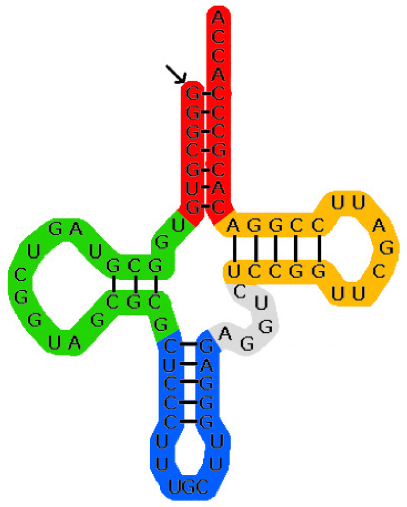
Single-stranded RNA molecules consist of a sequence of nucleotides connected by phosphordiester bonds. Nucleotides only differ by the bases involved, them being adenine, cytosine, guanine and uracil. The sequence of bases is called the primary structure of the molecule and is typically denoted as a word over the alphabet {A, C, G, U}. Additionally pairs of the bases can form hydrogen bonds (Typically adenine pairs with uracil and guanine pairs with cytosine. Other pairs are less stable and hence less common), thus folding the molecule to a complex three-dimensional layout called the tertiary structure. As determining the tertiary structure is computationally complex, it has proven convenient to first search for the secondary structure, for which only a subset of the hydrogen bonds is considered, so that the molecule can be modeled as a planar graph. Additionally so-called pseudoknots are eliminated, that is, there is no subsequence “first base of (hydrogen) bond 1 … first base of (hydrogen) bond 2 … second base of bond 1 … second base of bond 2” when traversing along the primary structure. See Figure 1 for an example of a secondary structure.
When abstracting from the primary structure, secondary structures are often denoted as words over the alphabet Σ = {(,|,)}, where a corresponding pair of parentheses represents a pair of bases connected by a hydrogen bond, while a | stands for an unpaired base. For example when starting transcription at the marked end the structure from Figure 1 would be denoted by the word
The oldest and most commonly used method for computing the secondary structure is to determine the structure with minimum free energy. This was first done by Nussinov et al. who, based on the observation that a high number of paired bases corresponds to a low free energy, used dynamic programming to find the structure with the highest number of paired bases in cubic time ([1]). While the energy models used today are much more sophisticated, taking into account, e.g., the types of bases involved in a pair, the types of bases located next to them, etc., the dynamic programming scheme has remained the same (e.g., [2]). A different approach is based on probabilistic modeling. An (ambiguous) stochastic context-free grammar (SCFG) that generates the primary structures is chosen such that the derivation trees for a given primary structure uniquely correspond to the possible secondary structures. The probabilities of this grammar are then trained either from molecules with known secondary structures or by expectation maximization ([3]). After this training the probabilities on the derivation trees as induced by the trained probabilities will model the probability of the corresponding secondary structures, assuming the training data was representative and the grammar is actually capable of modeling this distribution. Thus the most probable secondary structure (derivation tree) is computed as prediction ([3]). Many other approaches as well as extensions and modifications of the ones mentioned above have been suggested over the years. A recent overview can be found in [4]. With the exception of approaches that simulate the actual physical folding process (e.g., [5]) none of the existing prediction algorithms takes into account that in vivo the molecules grow sequentially and the folding takes place during their development. However it has been shown that this co-transcriptional folding has an effect on the resulting secondary structures (e.g., [6,7]). Since the simulation algorithms have the downside of being computationally expensive, it is desirable to add the effects of co-transcriptional folding into the traditional algorithms. In this paper we present an idea how this can be achieved for the SCFG approach. Due to co-transcriptional folding one would expect that the probability of two bases being paired depends on how far the bases are apart, and the probability of a part of the molecule forming a specific motif depends on how large the part of the molecule is. In SCFGs the distance between two paired bases (resp. the size of a motif) is just the size of the subword that results from the rule application introducing the base pair as first and last symbol (resp. starting building of the motif), assuming such a rule application exists. Thus to model this variability in the probabilities we suggest the concept of length-dependent SCFGs, which extend SCFGs such that rule probabilities now additionally depend on the size of the subword resulting from the rule application. We will present this extension formally in Section 2. In Sections 3 and 4 we show that existing training algorithms can easily be adapted to the new model without significant losses in performance. We have compared the prediction quality of the modified model with the conventional one for different grammars and sets of RNA. The results, presented in detail in Section 5, show that taking the lengths into account yields an improvement in most cases.
2. Formal Definitions
We assume the reader is familiar with basic terms of context-free grammars. An introduction can be found in ([8]).
Definition 1
A stochastic context-free grammar (SCFG) is a 5-tuple G = (I, T, R, S, P), where (I, T, R, S) is a context-free grammar (CFG) and P : R → [0, 1] is a mapping such that each rule r ∈ R is equipped with a probability P(r) satisfying ∀A ∈ I : ΣA → α∈R P(A → α) = 1.
Words are generated as for usual context-free grammars, the product of the probabilities of the production rules used in a parse tree Δ provides its probability P(Δ). The sum of the probabilities of all possible parse trees for a derivation A ⇒* α provides the probability P(A ⇒* α). Finally for a word w ∈ L(G) its probability is given by P(w) = P(S ⇒* w).
G is called consistent iff Σw∈L(G) P(w) = 1, i.e., it defines a probability distribution on L(G). To avoid the confusion of having two names for the same parameters, we will throughout this paper talk of probabilities on words and derivations even for (possibly) inconsistent grammars where there is no (guaranteed) probability distribution and the respective values thus would be more appropriately called weights.
As stated in the introduction we want to include the length of the generated subword in the rule probabilities in order to model that the probability of bases being paired depends on how far they are apart in the primary structure. To do this we first need to define the length of a rule application formally:
Definition 2
Let G = (I, T, R, S) a CFG, Δ a full-parse tree for G and A → α a specific rule application in Δ. The length of A → α is defined as the number of terminal symbols that label the leaves of the subtree rooted at this instance of A or equivalently the length of the subword eventually generated from A → α.
Now the straightforward way to make the rule probabilities depend on the length is to make the mapping P bivariate, the second parameter being the length of the rule application in question, and change the constraint on the probabilities to ∀A ∈ I ∀l ∈ ℕ : ΣA → α∈R P(A → α, l) = 1. We will use this idea, but in order to ensure that our modified versions of the training algorithms provide consistent grammars—like the original versions do for SCFGs—we need some technical additions to this idea.
First we note that that some combinations of rule and length can never occur in a derivation, e.g., a rule A → ∊ with length 1. It is reasonable to set the probability of such combinations to 0, which is what the training algorithms will do. This requires us to relax the condition to ΣA → α∈R P(A → α, l) ∈ {0, 1} in order to cover symbols for which no production can lead to a word of length l.
Further problems arise from the fact that while before P(A → α) expressed the probability that a parse tree with root A starts with rule A → α, now P(A → α, l) expresses the probability that a parse tree with root A starts with rule A → α, given that it generates a word of length l, but our model currently does not include the probabilities that a parse tree generates a word of a given length.
As an example consider the grammar characterised by the rules S → AA, A → aA and A → ∊. Here for each combination of intermediate symbol and length only one rule is applicable, leading to P(r, l) = 1 if r can lead to a word of length l and P(r, l) = 0 if it cannot. Thus for this grammar each parse tree will have “probability” 1 and each word will have a “probability” equal to its degree of ambiguity.
Checking the grammar more closely we find two points where the length of the word generated from an intermediate symbol is not determined when the symbol is introduced during a derivation: At the start of the derivation the length of the generated word is not predetermined and when the rule S → AA is applied to generate a word of length l there are l + 1 possible ways how the length can be distributed amongst the two symbols A.
Both cases can be countered by adding the proper probability distributions to the model. However while the start needs a single probability distribution Pℓ on the natural numbers (or a subset of them, if the grammar can not generate words of arbitrary length), the distribution of the lengths amongst the right side of the rule requires for each length l a set of l + 1 probabilities (generally
 (li−1) for a rule with i intermediate symbols on the right-hand side). Obviously storing these values with the grammar explicitly is not feasible unless we only want to consider short words. Approximating them with easily describable functions seems possible, but would potentially be difficult to automate and would not be covered by the considerations in Section 3. Thus we decided to use uniform distributions here.
Combining the above considerations length-dependent stochastic context-free grammars can be defined:
Definition 3
A length-dependent stochastic context-free grammar (LSCFG) is a 6-tuple G = (I, T, R, S, P, Pℓ), where (I, T, R, S) is a CFG, P : R × ℕ → [0, 1] is a mapping such that each pair of a rule r ∈ R and a length l ∈ ℕ is equipped with a probability P(r, l) satisfying ∀A ∈ I ∀l ∈ ℕ : ΣA → α∈R P(A → α, l) ∈ {0, 1} and Pℓ : ℕ → [0, 1] assigns probabilities to the lengths of words in L(G) such that .
For A → α ∈ R and l ∈ ℕ we define where cα,l is the number of different assignments of lengths to the symbols of α that satisfy:
Terminals are always assigned a length of 1.
Any intermediate symbol B is assigned a length i for which ∃w ∈ Ti : P(B ⇒* w) > 0.
The assigned lengths add up to l.
Words are generated as for usual context-free grammars. The probability P(Δ) of a parse tree Δ is then the product of the probabilities of all rule applications in Δ, each multiplied by pα,l, where α is the right hand side, l is the length of the respective rule application. The sum of the probabilities of all possible parse trees of a derivation A ⇒* α provides the probability P(A ⇒* α). Finally for a word w ∈ L(G) its probability is given by P(w) = Pℓ(|w|) · P(S ⇒* w).
G is called consistent iff Σw∈L(G) P(w) = 1, i.e., it defines a probability distribution on L(G).
This definition allows for the productions to be equipped with arbitrary probabilities as long as for any given pair (premise, length) they represent a probability distribution or are all 0. In the present paper we will however confine ourselves with grouping the lengths together in finitely many intervals, a rule having the same probability for lengths that are in the same interval. This allows for the probabilities to be stored as a vector and be retrieved in the algorithms without further computation. It is however, as we will see, still powerful enough to yield a significant improvement over non-length-dependent SCFGs with respect to the quality of the prediction.
Note 1
Since for bottom up parsing algorithms like CYK (see e.g., [9]) the length of the generated subword is determined by the position in the dynamic programming matrix, these algorithms will need no change other than adding the length as an additional parameter for probability lookup and multiplying the probabilities by pα,l in order to use them for LSCFGs.
For probabilistic Earley parsing ([10]) we have to regard that the length of the generated subword will only be known in the completion step. Thus for LSCFGs we have to multiply in the rule probability (and the factor pα,l) in this step instead of the prediction step, as is usually done.
Neither of these changes influence the run-time significantly. The same holds for the changes to the training algorithms explained at the beginning of the following section.
3. Estimating the Rule Probabilities
When given a set of training data
 of either full-parse trees of the grammar or words from the language generated by it, we want to train the grammar according to the maximum likelihood principle, i.e., choose rule probabilities such that
the grammar is consistent and
the likelihood L(
![Algorithms 04 00223i1]() , P) ≔ ∏t∈
, P) ≔ ∏t∈
![Algorithms 04 00223i2]() P(t) is maximised among all sets of probabilities that satisfy 1.
P(t) is maximised among all sets of probabilities that satisfy 1.
For (non-length-dependent) SCFGs it is well known how this can be achieved [11,12]:
If we are training from full-parse trees the relative frequencies with which the rules occur (among all rules with the same left-hand side) are a maximum-likelihood estimator.
When given a training set of words from L(G), the rule probabilities can be estimated using the inside-outside algorithm. This algorithm roughly works as follows:
Given an initial estimate of the rule probabilities it uses a modified version of the parsing algorithm to determine for each word w in the training set, each subword wi,j of w and each rule r ∈ R the total probability of all full-parse trees for w that derive wi,j in a subtree starting with r. Summing up these probabilities for all subwords it gets expected numbers of rule occurrences from which expected relative frequencies can be computed as in the case of given parse trees. By using these expected relative frequencies as a new estimate for the rule probabilities and iterating the procedure we are guaranteed to converge to a set of rule probabilities that gives a (local) maximum likelihood.
Both algorithms can easily be converted for LSCFGs: Instead of determining the (actual resp. expected) number of occurrences for each rule globally we determine separate counts for each length interval and use these to compute separate (expected) relative frequencies. This works since each occurrence (resp. probability of occurrence) is tied to a specific subword and thus associated a length.
What remains to be shown is that the modified versions of the algorithms still provide rule probabilities that yield consistent grammars and maximize the likelihood.
Our proof is based on the observation that an LSCFG is equivalent to an indexed grammar where each intermediate symbol A is split into a set of indexed symbols Ai and each rule A → α is split into a set of rules Ai → β, where β runs over all possible ways to index the intermediate symbols in α such that the sum of the indices plus the number of terminal symbols in β is i. In this grammar we can derive from each symbol Ai exactly those words that can be derived from A in the original grammar and have length i.
This indexed grammar is not context-free since it contains infinitely many intermediate symbols and rules but it can be converted into an SCFG by removing all symbols and rules with indices larger than some threshold n (thereby losing the possibility to generate words longer than n) and adding a new axiom S′ along with rules S′ → Si with probabilities Pℓ(i) (rescaled so they sum to 1).
For technical reasons the following formal definition will introduce one additional modification: The rules Ai → β are split into two rules Ai → Aα,i with the probability P(A → α, i) and Aα,i → β with the probability pα,i (where α is the unindexed counterpart of β). This reflects the distinction between choosing the symbols on the right-hand side and distributing the length amongst them introduced by our model.
Definition 4
For G = (I, T, R, S, P, Pℓ) a LSCFG and n ∈ ℕ the n-indexed SCFG corresponding to G is the SCFG Gn = (In, T, Rn, S′, Pn), where
,
,
,
Pn(Ai → Aα,i) = P(A → α, i),
Lemma 1
Let w ∈ Tm ∩ L(G), n ≥ m. Then w ∈ L(Gn) and there is a bijection between derivations A ⇒ w in G and derivations Am ⇒ w in Gn such that corresponding derivations have the same probability.
Additionally P(w) = Pn(w) · Σ0≤j≤n Pℓ(j).
Proof
The first claim is shown by structural induction on the derivations using the intuition given before Definition 4. The additional fact follows immediately from the first claim and the definition of the probabilities P(S′ → Si).
Thus the probability distribution on L(G) induced by Gn converges to the one induced by G as n → ∞. Furthermore since our training algorithms will set Pℓ(i) = 0 if the training data contains no word of length i we can consider training G equivalent to training Gn, n > maxt∈
 |t|, with the additional restrictions:
If i and j are in the same length interval Pn(Ai → Aα,i) = Pn(Aj → Aα,j) for each A → α ∈ R.
The second restriction obviously only applies if lengths are to be grouped into intervals as we will do in this paper. However not all such groupings can yield a consistent grammar. The following gives, as we will show afterwards, a sufficient condition that they do.
Definition 5
Let G = (I, T, R, S) a CFG, Q a partitioning of ℕ. We call Q consistent with G if it satisfies ∀q ∈ Q, i, j ∈ q : ∃A → α ∈ R, wi ∈ Ti : α ⇒* wi implies ∃wj ∈ Tj : α ⇒* wj.
Intuitively to satisfy this condition we may not group lengths i and j together if there is a rule that can lead to a word of length i but not to one of length j (or vice versa).
Note that the partitioning into sets of one element each, which corresponds to not grouping lengths into intervals at all is trivially consistent with each CFG G. Thus this case is implicitly included in the following definitions and proofs.
Definition 6
Let G = (I, T, R, S) a CFG, Q a partitioning of ℕ consistent with G and
a set of full-parse trees for G. For r ∈ R, i ∈ ℕ we denote by f(r, i,
) the number of applications of r in
with length i, by f(r,
) the total number of applications of r in
and by f(i,
) how many trees in
derive a word of length i.
A function P : R → [0, 1] is a relative frequency estimator for G on iff
A pair of functions (P : R × ℕ → [0, 1], Pℓ : ℕ → [0, 1]) is a relative frequency estimator for G on and Q iff
Lemma 2
Let G′ =(I, T, R, S) a CFG, Q a partitioning of ℕ consistent with G′,
a set of full-parse trees for G′ and (P, Pℓ) the relative frequency estimator for G′ on
and Q. Then G = (I, T, R, S, P, Pℓ) is consistent.
Proof
For n greater than the length of the longest word derived by a parse tree in
let Gn = (In, T, Rn, S′, Pn) the n-indexed SCFG corresponding to G. We show that
i = 0: Let
′ the images of the parse trees in
under the bijection from Lemma 1,
the relative frequency estimator for (In, T, Rn, S′) on
′ and
. By [12]:
.
By the definition of Gn a derivation A0 → ∊ can only consist of rules of the forms A0 → Aα,0 and Aα,0 → β. For the first kind the construction of the bijection in Lemma 1 guarantees that
. For the second type note that there is at most 1 way to distribute length 0 among the symbols of α ensuring that if Aα,0 occurs in
and if Aα,0 does not occur in
′ then the respective weights contribute to neither a0 nor
.
Thus proving the case i = 0.
i > 0: For each A ∈ I expanding ai along all possibilities for the first 2 derivation steps yields an equation , where each of the β contains at most one symbol Bi contributing a factor of bi along with an arbitrary number of other symbols (terminal or with smaller indices) contributing factors of 0 or 1 by the induction hypothesis.
By Definitions 4 and 6 we find Pn(β ⇒* w) = 0 implies Pn(Ai → Aα,i) · Pn(Aα,i → β) = 0. This allows us to simplify each equation to either ai = 0 or ai =ΣB∈I pi,AB · bi + (1 − ΣB∈I pi,AB), where .
Now let ci ≔ min{ai∣A ∈ I, ai > 0} and di ≔ max{ai∣A ∈ I}. Inserting these we find ci ≥ ΣB∈I pi,CB · ci + (1 − ΣB∈I pi,CB) giving ci ≥ 1 and di ≤ ΣB∈I pi,DB · di + (1 − ΣB∈I pi,DB) giving di ≤ 1, together proving the claim.
Theorem 3
Let G = (I, T, R, S) a CFG, Q a partitioning of ℕ consistent with G,
a set of full-parse trees for G′ and (P, Pℓ) the relative frequency estimator for G on
and Q. Then P is a maximum-likelihood estimator for the length-dependent rule-probabilities on G, R and Q.
Proof
Let P′ an arbitrary set of length-dependent probabilities on R. For each A ∈ I and q ∈ Q we define
On the right hand side of (1) the rightmost product is independent of the probabilities and all the other factors can be maximised independent of each other. Since each of these factors is described by an unrestricted probability distribution on its defining domain, Theorem 1 from [11] applies, stating that relative frequencies are a maximum likelihood estimator for their probabilities.
Thus by the definitions of and the and by Equation (1) the claim follows.
Theorem 4
Let G = (I, T, R, S) a CFG, Q a partitioning of ℕ consistent with G and
a set of full-parse trees for G. Then the inside-outside algorithm will converge to a set of rule probabilities that (locally or globally) maximises the likelihood of observing
.
Proof
From Theorem 11 of [11] and Theorem 3.
4. Determining the Most Probable Derivation
In order to find the most probable derivation for a given primary structure we decided to employ a probabilistic Earley parser, since it allows to use the grammars unmodified while the commonly used CYK algorithm requires the grammars to be transformed into Chomsky normal form.
A (non-probabilistic) Earley parser operates on lists of items (also called dotted productions), representing partial derivations. We will write (i : jX → αβ) if item list i, 0 ≤ i ≤ |w|, w the parsed word, contains the item jX → αβ with semantics: There is a (leftmost) derivation , a production X → αβ and a derivation . The item is considered to represent the partial derivation .
The parser is initialized with (0 : 0S′ → S), S′ a new symbol, S the axiom of the grammar, S′ → S a new production. Then the transitive closure with respect to the following operations is computed:
| Scanner: | If ∃ (i : kX → β1aβ2) and wi+ 1 = a, |
| add (i + 1 : kX → β1aβ2). | |
| Predictor: | If ∃ (i : kX → β1Aβ2) and A → α ∈ R, |
| add (i : iA → .α). | |
| Completer: | If ∃ (i : jY → ν.) and (j : kX → β1Yβ2), |
| add (i : kX → β1Yβ2). |
Intuitively the scanner advances the point past terminal symbols if they match the corresponding symbol of the parsed word, the predictor adds all the productions that might yield a valid extension of the following (nonterminal) symbol and the completer advances the point, if one actually did.
We then have w ∈ (G) ⇔ ∃ (|w| : 0S′ → S).
If we want to determine the most probable derivation of a word with respect to a SCFG (either length-dependent or not) we need to keep track of the probabilities of partial derivations. This can simply be done by adding them to the items as an additional parameter.
The initialisation then adds (0 : 0S′ → S, 1) and the operations change as follows:
| Scanner: | If ∃ (i : kX → β1aβ2, γ) and wi+1 = a, |
| add (i + 1 : kX → β1aβ2, γ). | |
| Predictor: | If ∃(i : kX → β1Aβ2, γ) and A → α ∈ R, |
| add (i : iA → .α, 1). | |
| Completer: | If ∃ (i : jY → ν., γ1), ∃ (j : kX → β1Yβ2, γ2) and |
| ∄ (i : kX → β1Yβ2, γ) | |
| where γ > γ′ ≔ γ1 · γ2 · P(Y → ν, i − j) · pν,i−j, | |
| add (i : kX → β1Yβ2, γ′). |
The modifications of scanner and predictor are straightforward. Since choosing the most probable sequence of steps for each partial derivation will lead to the most probable derivation overall, the completer maximises the overall probability by choosing the most probable alternative, whenever there are multiple possibilities for generating a subword.
If w ∈ (G) we will find (|w| : 0S′ → S, γ), where γ · Pℓ(|w|) is the probability of the most probable derivation of w.
Note 2
For a more detailed introduction of probabilistic Earley parsing as well as a proof of correctness and hints on efficient implementation see ([10]).
Differing from ([10]) we multiply in the rule probabilities P(f, i − j) during completion instead of prediction for the reasons mentioned in Note 1.
5. Application
In order to see if adding length-dependency actually improves the quality of the predictions of RNA secondary structures from stochastic context-free grammars, we used length-dependent and traditional versions of four different grammars to predict two sets of RNA molecules for which the correct secondary structure is already known. Both sets were split into a training set which was used to train the grammars and a benchmark set for which secondary structure were predicted using the trained grammars. We then compared these predicted structures to the structures from the database, computing two commonly used criteria to measure the quality:
Sensitivity (also called recall): The relative frequency of correctly predicted base pairs among base pairs that appear in the correct structure.
Specificity (also called precision): The relative frequency of correctly predicted base pairs among base pairs that have been predicted.
Both frequencies were computed over the complete set (instead of calculating individual scores for each molecule and taking the average of these).
5.1. Data
In [13] Dowell and Eddy compared the prediction quality of several different grammars as well as some commonly used programs that predict RNA secondary structures by minimizing free energy. We decided to use the same data so our results are directly comparable to theirs.
Their training set consists of 139 each large and small subunit rRNAs, the benchmark dataset contains 225 RNase Ps, 81 SRPs and 97 tmRNAs. Both sets are available from http://selab.janelia.org/software/conus/. Since it contains different types of RNA we will refer to this set as the mixed set for the remainder of this article.
Additionally we wanted to see if length-dependent prediction can further improve the prediction quality for tRNA which is already predicted well by conventional SCFGs.
In order to do so we took the tRNA database from [14], filtered out all sequences with unidentified bases and split the remaining data into a training set of 1285 sequences and a benchmark set of 1284 sequences.
5.2. Grammars
We used 4 different grammars for our experiments:
| G1: | S → bS ∣ aSâS ∣ ∊ |
| G2: | S → LS ∣ L |
| L → aLâ ∣ b | |
| F → aFâ ∣ LS | |
| G3: | S → AS ∣ bS ∣ b ∣ A |
| A → aAâ ∣ aRâ | |
| R → bT ∣ AT | |
| T → bT ∣ AT ∣ b ∣ A | |
| G4: | S → CAS ∣ C |
| C → bC ∣ ∊ | |
| A → aLâ | |
| L → aLâ ∣ M ∣ I ∣ bH ∣ aLâBb ∣ bBaLâ | |
| B → bB ∣ ∊ | |
| H → bH ∣ ∊ | |
| I → bJaLâKb | |
| J → bJ ∣ ∊ | |
| K → bK ∣ ∊ | |
| M → UaLâUaLâN | |
| N → UaLâN ∣ U | |
| U → bU ∣ ∊ |
In each of the grammars S is the start symbol, other capital letters denote nonterminal symbols and A → α ∣ β is used as a shorthand for A → α ∈ R and A → β ∈ R.
As we have stated before, the grammars are to generate the primary structures as words and encode the secondary structures in the derivation. Thus we have to distinguish (in the grammar) between terminal symbols representing unpaired bases and terminal symbols being part of a base pair. In the above grammars the former are denoted by the symbol b while the latter are denoted by pairs a, â.
Now simply introducing a rule for each combination of how the symbols a, â and b can be replaced by the terminal symbols would—especially in the case of G4—lead to a significant increase in the number of productions. To counter this the authors of [13] translated the concept of transition and emission probabilities from hidden Markov models to SCFGs. The transition probability then is the probability of choosing e.g. the rule scheme S → bS independent of which terminal symbol is used in place of b. The emission probability then is the probability that a given b is a placeholder, e.g. u independent of the rule which introduced the b.
In order to include this idea without having to extend the theory in Section 3 we left b in the grammar as a nonterminal and replaced all occurrences of aLâ in G4 (or the corresponding substrings in the other grammars) with A, adding rules that generate all (combinations of) terminal symbols a, c, g and u from these nonterminals.
G1 and G2 have been taken from [13], G1 being the simplest grammar in the comparison and G2, which originates from [3], being the grammar which achieved the best results. G2 and G3 both extend G1 based on the observation that a secondary structure will be more stable if it contains longer runs of immediately nested base pairs. They differ in the approach taken to get this into the model.
G4 has been taken from [15]. It models the decomposition that is used for minimum free energy prediction. Since a run of unpaired bases contributes differently to the free energy depending on the context it appears in, these runs are derived from a separate intermediate symbol (B, C, H, I, J or U) depending on the context with the intention of capturing these different contributions in the rule probabilities.
As we stated in Section 2 we implemented length-dependency such that we grouped the lengths into intervals, the rule probabilities changing only from one interval to the other but not within them.
Since the influence a change in length has on the probabilities most likely depends on the relative change rather than the absolute one, we decided to make the intervals longer as the subwords considered get longer. This also helps to keep the estimated probabilities accurate since naturally any training set will contain fewer data points per length as the length increases.
Aside from this consideration and the restrictions implied by Definition 5 (consistency of a set of intervals) there is no obvious criterion that helps with deciding on a set of intervals.
Thus we created several different sets ranging from approximately 10 to approximately 100 intervals, evaluating a subset of the prediction data with each of them. The results corresponded to our expectation that finer intervals would tend to improve the quality of prediction until at some point the amount of data available to estimate each probability would be too sparse and thus the quality would degrade. The following set of intervals yielded the best or close to the best results for all 4 grammars:
Lengths up to 40 were not grouped at all (i.e., for each of these lengths an individual set of probabilities was computed), lengths from 41 to 60 were grouped pairwise, then sets of three lengths up to 84, sets of four up to 100, sets of five up to 140, sets of ten up to 200, twenty lengths per set up to 300, [301; 330], [331; 360], [361; 390], [391; 430], [431; 470], [471; 510] and [511; ∞]. Since all structures in the benchmark sets are shorter than 500 bases the probabilities of the last interval did not influence the predictions.
At first glance it may seem surprising that on G4 the same number of intervals can be used as on the smaller grammars given the greater number of rules and thus greater number of probabilities that have to be trained. However a closer look shows that for all intermediate symbols in G4 except S, L and N there is at most one applicable rule for each length, leaving only 10 probabilities per interval to be actually determined by the training, which is the same number as for G3 and already less than the number of emission probabilities.
5.3. Observations and Dicussion
We did the training and prediction using a length-dependent version of the Earley-style-parser from [16]. The results of the benchmarks are listed in Table 1.
Looking at these results it is immediately apparent that the predictions from G1 are too bad to be of any use either without or with lengths. Additionally the higher complexity of G4 compared to G2 and G3 did not lead to an improvement in prediction quality.
Concerning the other grammars we note that adding length-dependency significantly improved the results on tRNA while they became worse on the mixed set.
A possible explanation for these results could be that the correct parameters for the folding are different for different types of RNA. In order to test this hypothesis we took the three types of RNA in the mixed benchmark set, splitting the molecules of each type into a training set containing 2/3 of them and a benchmark set containing the remaining molecules. On these three sets we again did the training and prediction for the grammars G2 and G3, them being the most likely candidates for future use. The results are listed in Table 2.
For each of the sets G3 with lengths performed best, backing our assumption. Additionally while the non-length-dependent versions of the grammar performed almost equal, the length-dependent version of G2 fell behind G3 significantly, indicating that length-dependent prediction is more sensitive to choice of grammar.
5.4. Runtime
The considerations in Note 1 lead to the assumption that both versions should take about the same time on a given grammar. This was confirmed during our experiments, with none of the versions being consistently faster, i.e., if there is a difference it was overshadowed by effects like system load.
Concerning the different grammars, predictions using G1 were faster than those for G2 by a factor of ∼ 1.5. Between G2 and G3 resp. G3 and G4 the factor was ∼ 2.
6. Conclusions
We introduced an extension to the concept of stochastic context-free grammars that allows the probabilities of the productions to depend on the length of the generated subword.
Furthermore we showed that existing algorithms that work on stochastic context-free grammars like training algorithms or determining the most likely parse-tree can easily be adapted to the new concept without significantly affecting their run-time or memory consumption.
Using the LSCFGs to predict the secondary structure of RNA molecules we found that if training and prediction are done on the same type of RNA, the grammar G3 with lengths always outperformed all of the non-length-dependent grammars we tested.
These results indicate that LSCFGs are indeed capable of giving better predictions than classic SCFGs. However further experiments will be needed to confirm these initial results on other data sets and determine good choices for grammar and length intervals.
6.1. Possible Other Applications
While our extension to the concept of stochastic context-free grammars stemmed from one specific application, it is not application specific. The concepts and methods presented in Sections 2-4 can immediately be applied to any other application where SCFGs are used as a model, e.g., natural language processing. From our limited insight in that field it appears possible that length-dependent grammars can successfully be applied there as well.
6.2. Language Theoretical Considerations
In addition to the applications, extending the concept of context-free grammars also gives rise to interesting questions in the field of formal language theory. The most obvious of these questions is if adding in length-dependencies changes the class of languages that can be generated. We have already been able to show this (For a simple example take the grammar with the productions S → A, A → aA ∣ ∊, with the first production restricted to lengths which are perfect squares. It generates {an2∣n ∈ ℕ} which is not context-free), leading us to the follow-up question what the properties of this new class of languages are. First results from this direction of research have been presented at a workshop ([17]) and a paper presenting more results is currently in preparation.

| Grammar | Mixed Set | tRNA Set | ||
|---|---|---|---|---|
| without | with | without | with | |
| lengths | lengths | |||
| G1 | 2 (2) | 2 (3) | 6 (6) | 6 (20) |
| G2 | 48 (45) | 35 (27) | 80 (80) | 96 (79) |
| G3 | 40 (48) | 40 (41) | 78 (81) | 95 (96) |
| G4 | 39 (47) | 22 (54) | 78 (83) | 84 (95) |
| Grammar | RNaseP Set | SRP Set | tmRNA Set | |||
|---|---|---|---|---|---|---|
| without | with | without | with | without | with | |
| lengths | lengths | lengths | ||||
| G2 | 50 (47) | 46 (36) | 57 (52) | 42 (34) | 39 (36) | 41 (23) |
| G3 | 47 (45) | 52 (53) | 57 (52) | 59 (54) | 38 (36) | 45 (59) |
Acknowledgments
We would like to thank the anonymous referees of the previous revisions for their helpful suggestions.
References
- Nussinov, R.; Pieczenik, G.; R'Griggs, J.; Kleitmann, D.J. Algorithms for loop matchings. SIAM J. Appl. Math. 1978, 35, 68–82. [Google Scholar]
- Zuker, M.; Stiegler, P. Optimal computer folding of large RNA sequences using thermodynamics and auxiliary information. Nucleic Acids Res. 1981, 9, 133–148. [Google Scholar]
- Knudsen, B.; Hein, J. RNA secondary structure prediction using stochastic context-free grammars and evolutionary history. Bioinformatics 1999, 15, 446–454. [Google Scholar]
- Andersen, E.S. Prediction and design of DNA and RNA structures. New Biotechnol. 2010, 27, 184–193. [Google Scholar]
- Xayaphoummine, A.; Bucher, T.; Isambert, H. Kinefold web server for RNA/DNA folding path and structure prediction including pseudoknots and knots. Nucleic Acids Res. 2005, 33, W605–W610. [Google Scholar]
- Boyle, J.; Robillard, G.T.; Kim, S. Sequential Folding of Transfer RNA. A nuclear magnetic resonance study of successively longer tRNA fragments with a common 5′ end. J. Mol. Biol. 1980, 139, 601–625. [Google Scholar]
- Meyer, I.; Miklos, I. Co-transcriptional folding is encoded within RNA genes. BMC Mol. Biol. 2004, 5, 10. [Google Scholar]
- Harrison, M.A. Introduction to Formal Language Theory; Addison-Wesley: Boston, MA, USA, 1978. [Google Scholar]
- Durbin, R.; Eddy, S.R.; Krogh, A.; Mitchison, G. Biological Sequence Analysis; Cambridge University Press: Cambridge, UK, 1998. [Google Scholar]
- Stolcke, A. An Efficient Probabilistic Context-Free Parsing Algorithm that Computes Prefix Probabilities. Comput. Linguist. 1995, 21, 165–201. [Google Scholar]
- Prescher, D. A Tutorial on the Expectation-Maximization Algorithm Including Maximum-Likelihood Estimation and EM Training of Probabilistic Context-Free Grammars. Available online: http://arxiv.org/pdf/cs/0412015 (accessed on 27 July 2011).
- Chi, T.; Geman, S. Estimation of Probabilistic Context-Free Grammars. Comput. Linguist. 1998, 24, 299–305. [Google Scholar]
- Dowell, R.D.; Eddy, S.R. Evaluation of several lightweight stochastic context-free grammars for RNA secondary structure prediction. BMC Bioinforma. 2004, 5, 71. [Google Scholar]
- Sprinzl, M.; Vassilenko, K.S.; Emmerich, J.; Bauer, F. Compilation of tRNA sequences and sequences of tRNA genes. Available online: http://www.uni-bayreuth.de/departments/biochemie/trna/ (accessed on 21 October 2011).
- Nebel, M.E. Identifying Good Predictions of RNA Secondary Structure. Proceedings of the Pacific Symposium on Biocomputing, Big Island, HI, USA, 6–10 January 2004.
- Wild, S. An Earley-style Parser for Solving the RNA-RNA Interaction Problem. B.Sc. Thesis, Kaiserslautern, Germany, 2010. [Google Scholar]
- Weinberg, F. Position-and-Length-Dependent Context-free Grammars. In Theorietag Automaten und Formale Sprachen 2009; Joran, M., Ludwig, S., Renate, W., Eds.; University Halle-Wittenberg: Halle, Germany, 2009. [Google Scholar]
© 2011 by the authors; licensee MDPI, Basel, Switzerland. This article is an open access article distributed under the terms and conditions of the Creative Commons Attribution license (http://creativecommons.org/licenses/by/3.0/.)
Share and Cite
Weinberg, F.; Nebel, M.E. Applying Length-Dependent Stochastic Context-Free Grammars to RNA Secondary Structure Prediction. Algorithms 2011, 4, 223-238. https://doi.org/10.3390/a4040223
Weinberg F, Nebel ME. Applying Length-Dependent Stochastic Context-Free Grammars to RNA Secondary Structure Prediction. Algorithms. 2011; 4(4):223-238. https://doi.org/10.3390/a4040223
Chicago/Turabian StyleWeinberg, Frank, and Markus E. Nebel. 2011. "Applying Length-Dependent Stochastic Context-Free Grammars to RNA Secondary Structure Prediction" Algorithms 4, no. 4: 223-238. https://doi.org/10.3390/a4040223