Goodness-of-Fit Tests For Elliptical and Independent Copulas through Projection Pursuit

Abstract
: Two goodness-of-fit tests for copulas are being investigated. The first one deals with the case of elliptical copulas and the second one deals with independent copulas. These tests result from the expansion of the projection pursuit methodology that we will introduce in the present article. This method enables us to determine on which axis system these copulas lie as well as the exact value of these very copulas in the basis formed by the axes previously determined irrespective of their value in their canonical basis. Simulations are also presented as well as an application to real datasets.1. Introduction
The need to describe the dependency between two or more random variables triggered the concept of copulas. We consider a joint cumulative distribution function (cdf) F on ℝd and its cdf margins F1, F2, …,Fd. A copula C is a function such that F = C(F1, F2, …, Fd). Sklar [1] is the first to lay the foundations of this new theory. Several parametric families of copulas have been defined, namely elliptical, archimedean, periodic copulas etc., see Joe [2] and Nelsen [3] as well as Appendix A for an overview of these families. Finding criteria to determine the best copula for a given problem can only be achieved through a goodness-of-fit (GOF) approach. So far several GOF copula approaches have been proposed in the literature, e.g., Carriere [4], Genest and Rémillard [5], Fermanian [6], Genest Quessy and Rémillard [7], Michiels and De Schepper [8], Genest Favre Béliveau and Jacques [9], Mesfioui Quessy and Toupin [10], Genest Rémillard and Beaudoin [11], Berg [12], Bücher and Dette [13], among others. However, the field is still at an embryonic stage which explains the current shortage in recommendations. In univariate distributions, the GOF assessment can be performed using for instance the well-known Kolmogorov test. In the multivariate field, there are fewer alternatives. A simple way to build GOF approaches for multivariate random variables is to consider multi-dimensional chi-square approaches, as in for example Broniatowski [14]. However, these approaches present feasibility issues for high dimensional problems due to the curse of dimensionality. In order to solve this, we recall some facts from the theory of projection pursuit.
The objective of projection pursuit is to generate one or several projections providing as much information as possible about the structure of the dataset regardless of its size. Once a structure has been isolated, the corresponding data are transformed through a Gaussianization. Through a recursive approach, this process is iterated to find another structure in the remaining data, until no further structure can be evidenced in the data left at the end. Friedman [15] and Huber [16] count among the first authors who introduced this type of approaches for evidencing structures. They each describe, with many examples, how to evidence such a structure and consequently how to estimate the density of such data through two different methodologies each. Their work is based on maximizing Kullback-Leibler divergence. In the present article, we will introduce a new projection pursuit methodology based on the minimisation of any ϕ-divergence greater than the L1-distance (ϕ-PP). We will show that this algorithm presents the extra advantage of being robust and fast from a numerical standpoint. Its key rationale lies in the fact that it allows not only to carry out GOF tests for elliptical and independent copulas but also to determine the axis system upon which these very copulas are based. The exact expression of these copulas in the basis constituted by these axes can therefore be derived.
This paper is organised as follows: Section 2 contains preliminary definitions and properties. In Section 3, we present in details the ϕ-projection pursuit algorithm. In Section 4, we present our first results. In Section 5, we introduce our tests. In Section 6, we provide three simulations pertaining to the two major situations described herein and we will study a real case.
2. Basic theory
2.1. An Introduction to Copulas
In this section, we recall the concept of copula. We will also define the family of elliptical copulas through a brief reminder of elliptical distributions—see Appendix A for an overview of other families.
Sklar's Theorem
First, let us define a copula in ℝd.
Definition 2.1
A d-dimensional copula is a joint cumulative distribution function C defined on [0, 1]d, with uniform margins.
The following theorem explains in what extent a copula does describe the dependency between two or more random variables.
Theorem 2.1 (Sklar [1])
Let F be a joint multivariate distribution with margins F1, …, Fd, then, there exists a copula C such that
If marginal cumulative distributions are continuous, then the copula is unique. Otherwise, the copula is unique on the range of values of the marginal cumulative distributions.
Remark 2.1
First, for any copula C and any ui in [0, 1], 1 ≤ i ≤ d, we have
We set the independent copula Π as , for any ui in [0, 1], 1 ≤ i ≤ d.
Moreover, we define the density of a copula as the density associated with the cdf C, which we will name as c:
Definition 2.2
Whenever there exists, the density of C is defined by , for any ui in [0, 1], 1 ≤ i ≤ d.
Finally, let us present several examples of copulas (see also Appendix A to find an overview).
Example 2.1
The Gaussian copula Cρ (in ℝ2):
Defining Ψρ as the standard bivariate normal cumulative distribution function with ρ correlation, the Gaussian copula function is
The Student copula Cρ (in ℝ2):
Defining Tρ,k as the standard bivariate student cumulative distribution function with ρ as the correlation coefficient and with k as the degree of freedom of the distribution, the Student copula function is
The Elliptical copula :
Similarly as above, elliptical copulas are the copulas of elliptical distributions (an overview is provided in Appendix A).
2.2. Brief Introduction to the ϕ-Projection Pursuit Methodology (ϕ-PP)
Let us first introduce the concept of ϕ-divergence.
The Concept of ϕ-Divergence
Let φ be a strictly convex function defined by , and such that φ(1) = 0. We define a ϕ-divergence of P from Q, where P and Q are two probability distributions over a space Ω such that Q is absolutely continuous with respect to P-by
Throughout this article, we will also assume that φ(0) < ∞, that φ′ is continuous and that this divergence is greater than the L1 distance—see also Appendix B page 109.
Functioning of the Algorithm
Let f be a density on ℝd. We consider an instrumental density g with the same mean and variance as f. We start with performing the Dϕ(g, f) = 0 test; should this test turn out to be positive, then f = g and the algorithm stops, otherwise, the first step of our algorithm consists in defining a vector a1 and a density g(1) by
In our second step, we replace g with g(1) and we repeat the first step, and so on. By iterating this process, we end up obtaining a sequence (a1, a2, …) of vectors in and a sequence of densities g(i).
Remark 2.2
First, to obtain an approximation of f, we stop our algorithm when the divergence equals zero, i.e., we stop when Dϕ(g(j), f) = 0 since it implies g(j) = f with j ≤ d, or when our algorithm reaches the dth iteration, i.e., we approximate f with g(d).
Second, we get Dϕ(g(0), f) ≥ Dϕ(g(1), f) ≥ …‥ ≥ 0 with g(0) = g.
Finally, the specific form of the relationship (2.2) implies that we deal with M-estimation. We can therefore state that our method is robust—see Sections 6, Yohai [19], Toma [20] as well as Huber [21].
The main steps of the present algorithm have been summarized in Table 1.
At present, let us study the following example:
Example 2.2
Let f be a density defined on ℝ3 by f(x1, x2, x3) = n(x1, x2)h(x3), with n being a bi-dimensional Gaussian density, and h being a non-Gaussian density. Let us also consider g, a Gaussian density with the same mean and variance as f.
Since g(x1, x2/x3) = n(x1, x2), we have as f3 = h, i.e., the function reaches zero for e3 = (0, 0, 1)′, where f3 and g3 are the third marginal densities of f and g respectively. We therefore obtain g(x1, x2/x3) = f(x1, x2/x3).
To recapitulate our method, if Dϕ(g, f) = 0, we derive f from the relationship f = g; whenever a sequence (ai)i=1,…j, j < d, of vectors in defining g(j) and such that Dϕ(g(j), f) = 0 exists, then i.e., f coincides with g on the complement of the vector subspace generated by the family {ai}i=1,…,j—see also Section 3 for a more detailed explanation.
In the remaining of our study of the algorithm, after having clarified the choice of g, we will consider the statistical solution to the representation problem, assuming that f is unknown and that X1, X2,…Xm are i.i.d. with density f. We will provide asymptotic results pertaining to the family of optimizing vectors ak,m—which we will define more precisely below—as m goes to infinity. Our results also prove that the empirical representation scheme converges towards the theoretical one.
3. The Algorithm
3.1. The Model
Let f be a density on ℝd. We assume there exists d non-null linearly independent vectors aj, with 1 ≤ j ≤ d, of ℝd, such that
We define g as an elliptical distribution with the same mean and variance as f.
For simplicity, let us assume that the family {aj}1≤j≤d is the canonical basis of ℝd:
The very definition of f implies that (Xj+1, …, Xd) is independent from (X1, …, Xj). Hence, the density of (Xj+1, …, Xd) given (X1, …, Xj) is n.
Let us assume that Dϕ(g(j), f) = 0, for some j ≤ d. We then get , since, by induction, we have .
Consequently, lemma C.1 and the fact that the conditional densities with elliptical distributions are also elliptical, as well as the above relationship, lead us to infer that . In other words, f coincides with g on the complement of the vector subspace generated by the family {ai}i=1,…,j.
Now, if the family {aj}1≤j≤d is no longer the canonical basis of ℝd, then this family is again a basis of ℝd. Hence, lemma C.2 implies that
The end of our algorithm implies that f coincides with g on the complement of the vector subspace generated by the family {ai}i=1,…,j. Therefore, the nullity of the ϕ-divergence provides us with information on the density structure.
In summary, the following proposition clarifies our choice of g which depends on the family of distribution one wants to find in f :
Proposition 3.1
With the above notations, Dϕ(g(j), f) = 0 is equivalent to
More generally, the above proposition defines the co-support of f as the vector space generated by the vectors a1, …, aj.
Definition 3.1
Let f be a density on ℝd. We define the co-vectors of f as the sequence of vectors a1, …, aj which solves the problem Dϕ(g(j), f) = 0 where g is an elliptical distribution with the same mean and variance as f. We define the co-support of f as the vector space generated by the vectors a1, …, aj.
Remark 3.1
Any (ai) family defining f as in (3.1) is an orthogonal basis of ℝd—see lemma C.3
3.2. Stochastic Outline of Our Algorithm
Let X1, X2,‥,Xm (resp. Y1, Y2,‥,Ym) be a sequence of m independent random vectors with the same density f (resp. g). As customary in nonparametric ϕ-divergence optimizations, all estimates of f and fa, as well as all uses of Monte Carlo methods are being performed using subsamples X1, X2,‥,Xn and Y1, Y2,‥,Yn—extracted respectively from X1, X2,‥,Xm and Y1, Y2,‥,Ym—since the estimates are bounded below by some positive deterministic sequence θm—see Appendix D.
Let ℙn be the empirical measure based on the subsample X1, X2,.,Xn. Let fn (resp. fa,n for any a in be the kernel estimate of f (resp. fa), which is built from X1, X2,‥,Xn (resp. a⊤X1, a⊤X2,‥,a⊤Xn).
As defined in Section 2.2, we consider the following sequences (ak)k≥1 and (g(k))k≥1 such that
The stochastic setting up of the algorithm uses fn and instead of f and g(0) = g—since g is known. Thus, at the first step, we build the vector ǎ1 which minimizes the ϕ-divergence between fn and and which estimates a1. First, since proposition D.1 and lemma C.4 show how the infimum of the criteria (or index)
Now, from the second step and as defined in Section 2.2, we derive the fact that the density g(2–1) is unknown. Consequently, once again, the samples have to be truncated.
All estimates of f and fa (resp. g(1) and ) are being performed using a subsample X1, X2,…,Xn (resp. ) extracted from X1, X2,…,Xm (resp. , which is a sequence of m independent random vectors with same density g(1)) such that the estimates are bounded below by some positive deterministic sequence θm—see Appendix D.
Let ℙn be the empirical measure of the subsample X1, X2,…,Xn. Let fn (resp. for any a in ) be the kernel estimate of f (resp. g(1) and fa as well as ) which is built from X1, X2,…,Xn (resp. and a⊤X1, a⊤X2,…,a⊤Xn as well as ).
The stochastic setting up of the algorithm uses fn and instead of f and g(1). Thus, we build the vector ǎ2, which minimizes the ϕ-divergence between fn and , since g(1) and are unknown—and which estimates a2. First, since proposition D.1 and lemma C.4 show how the infimum of the criteria (or index)
And so on, we end up obtaining a sequence (ǎ1, ǎ2, …) of vectors in estimating the co-vectors of f and a sequence of densities such that estimates g(k) through theorem 4.1.
Let us now summarize the main steps of the stochastic implementation of our algorithm (the dual representation of the estimators will be further detailed in Table 2 below).
4. Results
4.1. Hypotheses on f
In this paragraph, we define the set of hypotheses on f which could possibly be of use in our work. Discussion on several of these hypotheses can be found in Appendix E.
In the remaining of this section, for legibility reasons, we replace g with g(k−1). Let
Similarly as in chapter V of Van der Vaart [22], let us define :
(A1) : For all ε > 0, there is η > 0, such that for all c ∈ ΘDϕ verifying ‖c − ak‖ ≥ ε, we have PM(c, a) − η > PM(ak, a), with a ∈ Θ.
(A2) : ∃ Z < 0, n0 > 0 such that (n ≥ n0 ⇒ supa∈Θ supc∈{ΘDϕ}c ℙnM(c, a) < Z)
(A3) : There exists V, a neighbourhood of ak, and H, a positive function, such that, for all c ∈ V, we have |M(c, ak, x)| ≤ H(x)(P − a.s.) with PH < ∞,
(A4) : There exists V, a neighbourhood of ak, such that for all ε, there exists a η such that for all c ∈ V and a ∈ Θ, verifying ‖a − ak‖ ≥ ε, we have PM(c, ak) < PM(c, a) − η.
Putting , let us consider now four new hypotheses:
(A5) : and are finite and the expressions and Iak exist and are invertible.
(A6) : There exists k such that PM(ak, ak) = 0.
(A7) : (VarP(M(ak, ak)))1/2 exists and is invertible.
(A0) : f and g are assumed to be positive and bounded and such that K(g, f) ≥ ∫ |f(x) − g(x)|dx where K is the Kullback-Leibler divergence.
Estimation of the First Co-Vector of f
Let be the class of all positive functions r defined on ℝ and such that g(x)r(a⊤x) is a density on ℝd for all a belonging to . The following proposition shows that there exists a vector a such that minimizes Dϕ(gr, f) in r:
Proposition 4.1
There exists a vector a belonging to such that
Following Broniatowski [33], let us introduce the estimate of , through .
Proposition 4.2
Let ǎ be such that .
Then, ǎ is a strongly convergent estimate of a, as defined in proposition 4.1.
Let us also introduce the following sequences (ǎk)k≥1 and , for any given n—see Section 3.2—such that
ǎk is an estimate of ak as defined in proposition 4.2 with instead of g, is defined by , , i.e., .
We also note that is a density.
Convergence Study at the kth Step of the Algorithm:
In this paragraph, we show that the sequence (ǎk)n converges towards ak and that the sequence converges towards g(k).
Let čn(a)= arg supc∈Θ ℙnM(c, a), with a ∈ Θ, and γ̌n = arg infa∈Θ supc∈Θ ℙnM(c, a). We state
Proposition 4.3
Both supa∈Θ ‖čn(a) – ak‖ and γ̌n converge toward ak a.s.
Finally, the following theorem shows that converges almost everywhere towards g(k):
Theorem 4.1
It holds a.s.
Testing of the Criteria
In this paragraph, through a test of our criteria, namely , we build a stopping rule for this procedure. First, the next theorem enables us to derive the law of our criteria:
Theorem 4.2
For a fixed k, we have , where k represents the kth step of our algorithm and where I is the identity matrix in ℝd.
Note that k is fixed in theorem 4.2 since γ̌n = arg inf a∈Θ supc∈Θ ℙnM(c, a) where M is a known function of k—see Section 4.1. Thus, in the case when , we obtain
Corollary 4.1
We have .
Hence, we propose the test of the null hypothesis
versus the alternative .
Based on this result, we stop the algorithm, then, defining ak as the last vector generated, we derive from corollary 4.1 a α-level confidence ellipsoid around ak, namely , where is the quantile of a α-level reduced centered normal distribution and where ℙn is the empirical measure arising from a realization of the sequences (X1, …, Xn) and (Y1, …, Yn).
Consequently, the following corollary provides us with a confidence region for the above test:
Corollary 4.2
k is a confidence region for the test of the null hypothesis (H0) versus (H1).
5. Goodness-of-Fit Tests
5.1. The Basic Idea
Let f be a density defined on ℝ2. Let us also consider g, a known elliptical density with the same mean and variance as f. Let us also assume that the family (ai) is the canonical basis of ℝ2 and that Dϕ(g(2), f) = 0.
Hence, since lemma C.1 page 110 implies that if j ≤ d, we then have . Moreover, we get f with g(2) = f, as derived from property B.1 page 110.
Consequently, , i.e., , and then where Cf (resp. Cg) is the copula of f (resp. g).
More generally, if f is defined on ℝd, then the family (ai) is once again free (see lemma C.5), i.e., the family (ai) is once again a basis of ℝd. The relationship Dϕ(g(d), f) = 0 therefore implies that g(d) = f, i.e., for any x ∈ ℝd, since lemma C.1 page 110 implies that if k ≤ d. In other words, for any x ∈ ℝd, it holds
Finally, putting A = (a1, …, ad) and defining vector y (resp. density f̃, copula C̃f of f̃, density g̃, copula C̃g of g̃) as the expression of vector x (resp. density f, copula Cf of f, density g, copula Cg of g) in basis A, then, the following proposition provides us with the density associated with the copula of f as being equal to the density associated with the copula of g in basis A :
Proposition 5.1
With the above notations, should a sequence (ai)i=1,…d of not null vectors in defining g(d) and such that Dϕ(g(d), f) = 0 exist, then .
5.2. With the Elliptical Copula
Let f be an unknown density defined on ℝd. The objective of the present section is to determine whether the copula of f is elliptical. We thus define an instrumental elliptical density g with the same mean and variance as f, and we follow the procedure of Section 3.2. As explained in Section 5.1, we infer from proposition 5.1 that the copula of f equals the copula of g when Dϕ(g(d), f) = 0, i.e., when ad is the last vector generated from the algorithm and when (ai) is the canonical basis of ℝd. Thus, in order to verify this assertion, corollary 4.1 page 96 provides us with a α-level confidence ellipsoid around this vector, namely
Consequently, keeping the notations introduced in Section 5.1, we perform a statistical test of the null hypothesis
Since, under (H0), we have Dϕ(g(d), f) = 0, then the following theorem provides us with a confidence region for this test.
Theorem 5.1
The set d is a confidence region for the test of the null hypothesis (H0) versus the alternative (H1).
Remark 5.1
1/If Dϕ(g(k), f) = 0, for k < d, then we reiterate the algorithm until g(d) is created in order to obtain a relationship for the copula of f.
2/If the ai do not constitute the canonical basis, then keeping the notations introduced in Section 5.1, our algorithm meets the test:
5.3. With the Independent Copulas
Let f be a density on ℝd and let X be a random vector with f as density. The objective of this section is to determine whether f is the product of its margins, i.e., whether the copula of f is the independent copula. Let g be an instrumental product of univariate Gaussian density—with diag(Var(X1),…, Var(Xd)) as covariance matrix and with the same mean as f. As explained at Section 5.2, we follow the procedure described at Section 3.2, i.e., proposition 5.1 infers that the copula of f is the independent copula when Dϕ(g(d), f) = 0, we then perform a statistical test of the null hypothesis:
Since, under (H0), we have Dϕ(g(d), f) = 0, the following theorem provides us with a confidence region for our test.
Theorem 5.2
Keeping the notations of Section 5.2, the set d is a confidence region for the test of the null hypothesis (H0) versus the alternative (H1).
Remark 5.2
(1) As explained in Section 5.2, if Dϕ(g(k), f) = 0, for k < d, we reiterate the algorithm until g(d) is created in order to derive a relationship for the copula of f.
(2) If the ai do not constitute the canonical basis, then keeping the notations of Section 5.1, our algorithm meets the test:
Thus, our method enables us to determine if the copula of f is the independent copula in the (a1, …, ad) basis.
5.4. Study of the Subsequence (g(k′)) Defined by Dϕ(g(k′), f) = 0 for Any k′
Let
 be the set of non-negative integers defined by
, where q—such that q ≤ d—is its cardinal. In the present section, our goal is to study the subsequence (g(k′)) of the sequence (g(k))k=1‥d defined by Dϕ(g(k′), f) = 0 for any k′ belonging to
.
be the set of non-negative integers defined by
, where q—such that q ≤ d—is its cardinal. In the present section, our goal is to study the subsequence (g(k′)) of the sequence (g(k))k=1‥d defined by Dϕ(g(k′), f) = 0 for any k′ belonging to
.
First, we have:
Dϕ(g(d), f) = 0 ⇔ g(d) = f, through property B.1
, as explained in Section 5.2
, which amounts to the previous relationship written in the A = (a1, …, ad) basis with the notations introduced in Section 5.2.
Moreover, defining as the previous integer , in the space {1, …, d}, with i > 1, and as explained in Section 3.1, the relationship Dϕ(g(k′), f) = 0 implies that
Hence, we can infer that
The following theorem explicitly describes the form of the f copula in the A = (a1, …, ad) basis:
Theorem 5.3
Defining C̃fi,j as the copula of f̃i,j and keeping the notations introduced in Sections 5.1 and 5.4, it holds
Remark 5.3
If there exists i such that i < d and , then the notation means . Thus, if, for any k, we have Dϕ(g(k), f) = 0, then, for any i < d, we have , i.e., we have , where f̃k is the kth marginal density of f̃.
At present, using relationship 5.2 and remark 5.3, the following corollary gives us the copula of f as equals to 1 in the {a1, …, ad} basis when, for any k, Dϕ(g(k′), f) = 0:
Corollary 5.1
In the case where, for any k, Dϕ(g(k), f) = 0, it holds:
6. Simulations
Let us examine three simulations and an application to real datasets. The first simulation studies the elliptical copula and the second studies the independent copula. In each simulation, our program will aim at creating a sequence of densities (g(j)), j = 1,‥,d such that g(0) = g, g(j) = g(j−1)faj/[g(j−1)]aj and Dϕ(g(d), f) = 0, where Dϕ is a divergence—see Appendix B for its definition—and , for all j = 1, …, d. We will therefore perform the tests introduced at theorems 5.1 and 5.2. Finally, the third simulation compares the optimisations obtained, when we execute the process with, each time, a new ϕ-divergence.
Simulation 6.1
We are in dimension 2(=d), and we use the χ2 divergence to perform our optimisations. Let us consider a sample of 50(=n) values of a random variable X with a density law f defined by :
Let us generate then a Gaussian random variable Y with a density—that we will name as g—presenting the same mean and variance as f.
We theoretically obtain k = 2 and (a1, a2) = ((1, 0), (0, 1)).
To get this result, we perform the following test:
Then, theorem 5.1 enables us to verify (H0) by the following 0.9(=α) level confidence ellipsoid
Results of this optimisation can be found in Table 3 and Figure 1.
Therefore, we can conclude that H0 is verified.
Simulation 6.2
We are in dimension 2(=d), and we use the χ2 divergence to perform our optimisations.
Let us consider a sample of 50(=n) values of a random variable X with a density law f defined by
Let g be an instrumental product of univariate Gaussian densities with diag(V ar(X1), …, V ar(Xd)) as covariance matrix and with the same mean as f.
We theoretically obtain k = 2 and (a1, a2) = ((1, 0), (0, 1)). To get this result, we perform the following test:
Then, theorem 5.2 enables us to verify (H0) by the following 0.9(=α) level confidence ellipsoid
Results of this optimisation can be found in Table 4 and Figure 2.
Therefore, we can conclude that .
Simulation 6.3
(On the choice of a ϕ-divergence). In this paragraph, we perform our algorithm several times. We first use several ϕ-divergences (see Appendix B for their definitions and their notations). We then perform a sensitivity analysis by varying the number n of simulated variables. Finally we introduce outliers.
At present, we consider a sample of n values of a random variable X with a density f defined by f(x) = Laplace(x1).Gumbel(x0),
where the Gumbel distribution parameters are (1, 2) and where the Laplace distribution parameters are 4 and 3. In theory, we get a1 = (0, 1) and a2 = (1, 0). Then, following the procedure of the first simulation, we get

| n = 50 | Outliers = 0 | Time | Outliers = 2 | Time |
|---|---|---|---|---|
| Relative Entropy | (0.10, 0.83) (1.13, 0.11) | 30 mn | (0.1, 0.8) (0.80, 0.024) | 43 mn |
| χ2-divergence | (0, 0.8) (1.021, 0.09) | 22 mn | (0.12, 0.79) (0.867, −0.104) | 31 mn |
| Hellinger distance | (0.1, 0.9) (0.91, 0.15) | 35 mn | (0.1, 0.85) (0.81, 0.14) | 46 mn |
| n = 100 | Outliers = 0 | Time | Outliers = 5 | Time |
|---|---|---|---|---|
| Relative Entropy | (0.09, 0.89) (1.102, 0.089) | 50 mn | (0.1, 0.88) (1.15, 0.144) | 60 mn |
| χ2-divergence | (0, 0.9) (0.97, −0.1) | 43 mn | (−0.1, 0.9) (0.87, 0.201) | 52 mn |
| Hellinger distance | (0.1, 0.91) (0.93, −0.11) | 57 mn | (−0.05, 1.1) (0.79, 0.122) | 62 mn |
| n = 500 | Outliers = 0 | Time | Outliers = 25 | Time |
|---|---|---|---|---|
| Relative Entropy | (0, 1.07) (1.1, −0.05) | 107 mn | (0.13, 0.75) (0.79, 0.122) | 121 mn |
| χ2-divergence | (0, 0.95) (1.12, −0.02) | 91 mn | (0.15, 0.814 (0.922, 0.147) | 103 mn |
| Hellinger distance | (−0.01, 0.95) (1.01, −0.073) | 100 mn | (−0.17, 1.3) (0.973, 0.206) | 126 mn |
Remark 6.1
We have worked with a calculator presenting the following characteristics :
- -
Processor : Mobile AMD 3000+,
- -
Memory RAM : 512 DDR,
- -
Windows XP.
Our method, which uses the χ2 as ϕ-divergence, is faster and its performance is as good if not better than any other divergence method.
This results from the fact that the projection index (or criteria) of χ2 is a second degree polynomial. It is consequently easier and faster to assess. Moreover, these simulations illustrate the robustness of our method.
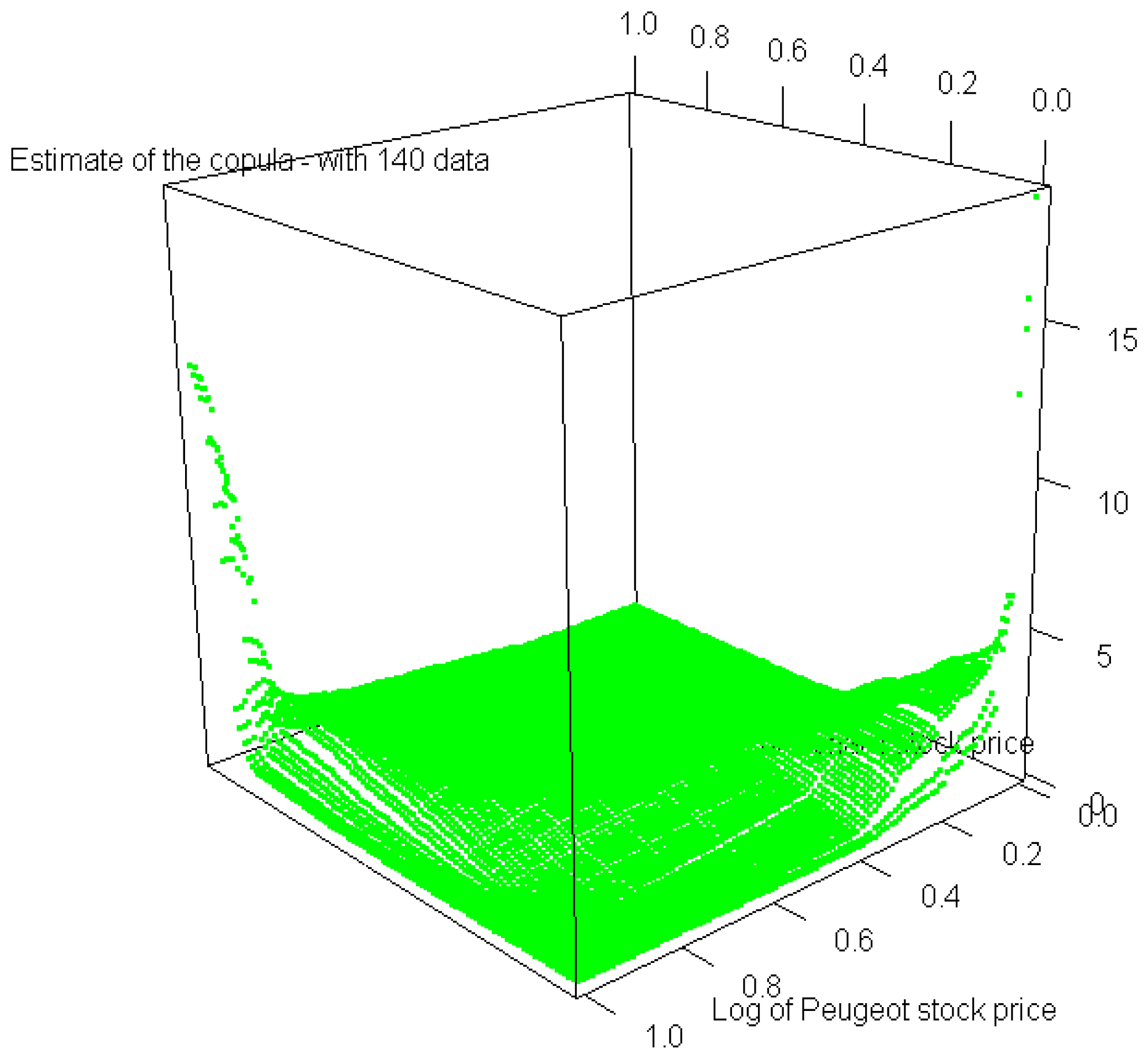
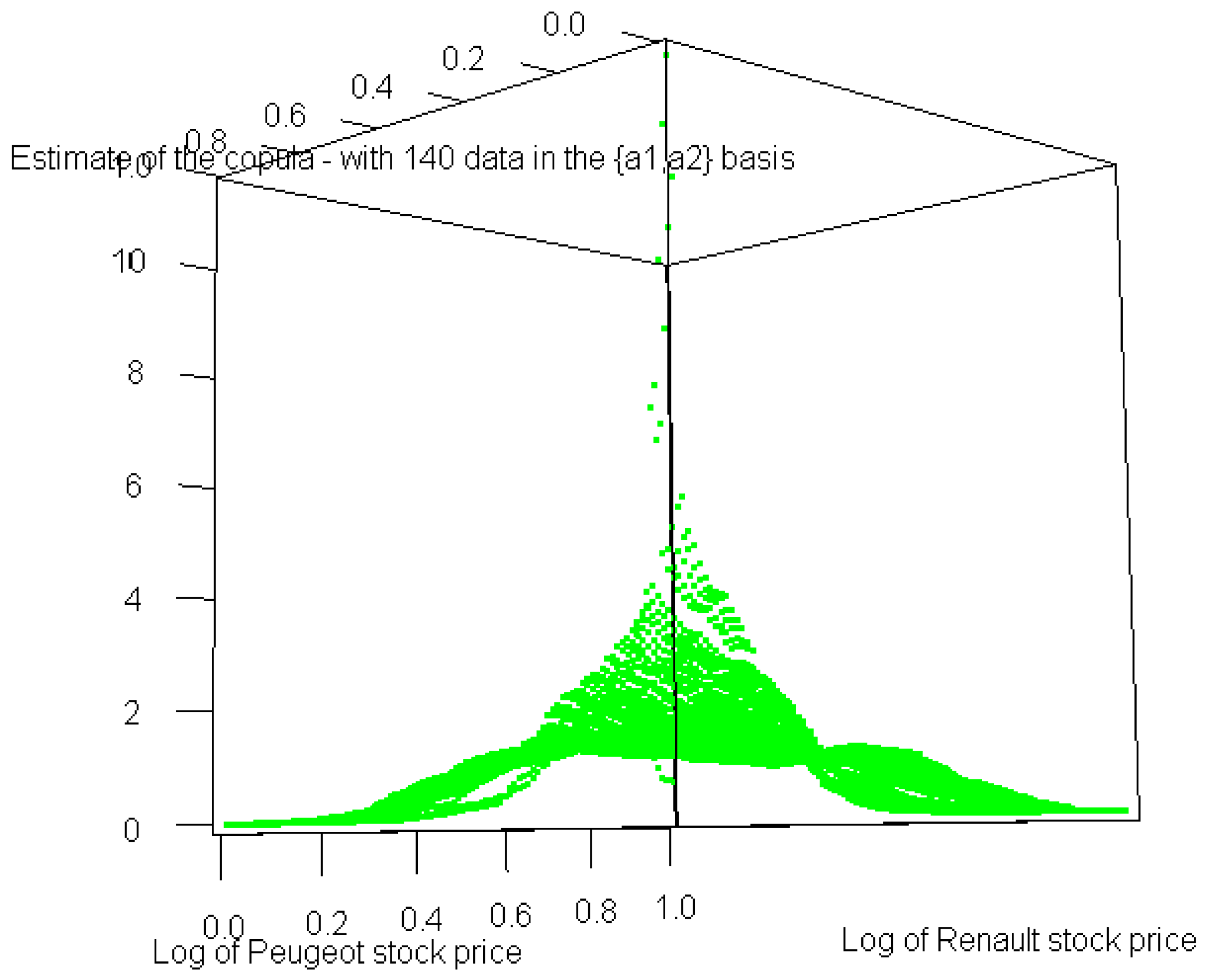
6.1. Application to Real Datasets
Let us for instance study the moves in the stock prices of Renault and Peugeot from January 4, 2010 to July 25, 2010. We thus gather 140(=n) data from these stock prices, see Table 7 and Table 8 below.
Let us also consider X1 (resp. X2) the random variable defining the stock price of Renault (resp. Peugeot). We will assume—as it is commonly done in mathematical finance—that the stock market abides by the classical hypotheses of the Black-Scholes model—see Black and Scholes [34].
Consequently, X1 and X2 each present a log-normal distribution as probability distribution.
Let f be the density of vector (ln(X1), ln(X2)), let us now apply our algorithm to f with the Kullback-Leibler divergence as ϕ-divergence. Let us generate then a Gaussian random variable Y with a density—that we will name as g—presenting the same mean and variance as f.
We first assume that there exists a vector a such that .
In order to verify this hypothesis, our reasoning will be the same as in Simulation 6.1. Indeed, we assume that this vector is a co-factor of f. Consequently, corollary 4.2 enables us to estimate a by the following 0.9(=α) level confidence ellipsoid
Numerical results of the first projection are summarized in Table 5.
Therefore, our first hypothesis is confirmed.
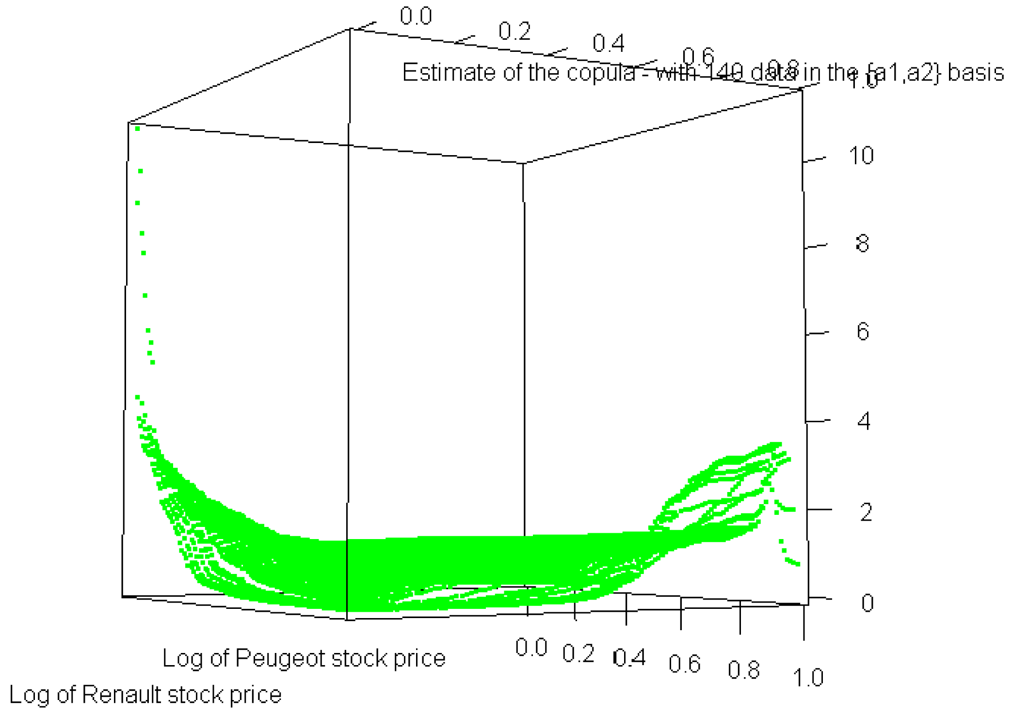
However, our goal is to study the copula of (ln(X1), ln(X2)). Then, as explained in Section 5.4, we formulate another hypothesis assuming that there exists a vector a such that .
In order to verify this hypothesis, we use the same reasoning as above. Indeed, we assume that this vector is a co-factor of f. Consequently, corollary 4.2 enables us to estimate a by the following 0.9(=α) level confidence ellipsoid . Numerical results of the second projection are summarized in Table 6.
Therefore, our second hypothesis is confirmed.
In conclusion, as explained in corollary 5.1, the copula of f is equal to 1 in the {a1, a2} basis.
6.2. Critics of the Simulations
In the case where f is unknown, we will never be sure to have reached the minimum of the ϕ-divergence: the simulated annealing method has been used to solve our optimisation problem, and therefore it is only when the number of random jumps tends in theory towards infinity that the probability to get the minimum tends to 1. We also note that no theory on the optimal number of jumps to implement does exist, as this number depends on the specificities of each particular problem.
Moreover, we choose the for the AMISE of the two simulations. This choice leads us to simulate 50 random variables—see Scott [23] page 151, none of which have been discarded to obtain the truncated sample.
This has also been the case in our application to real datasets.
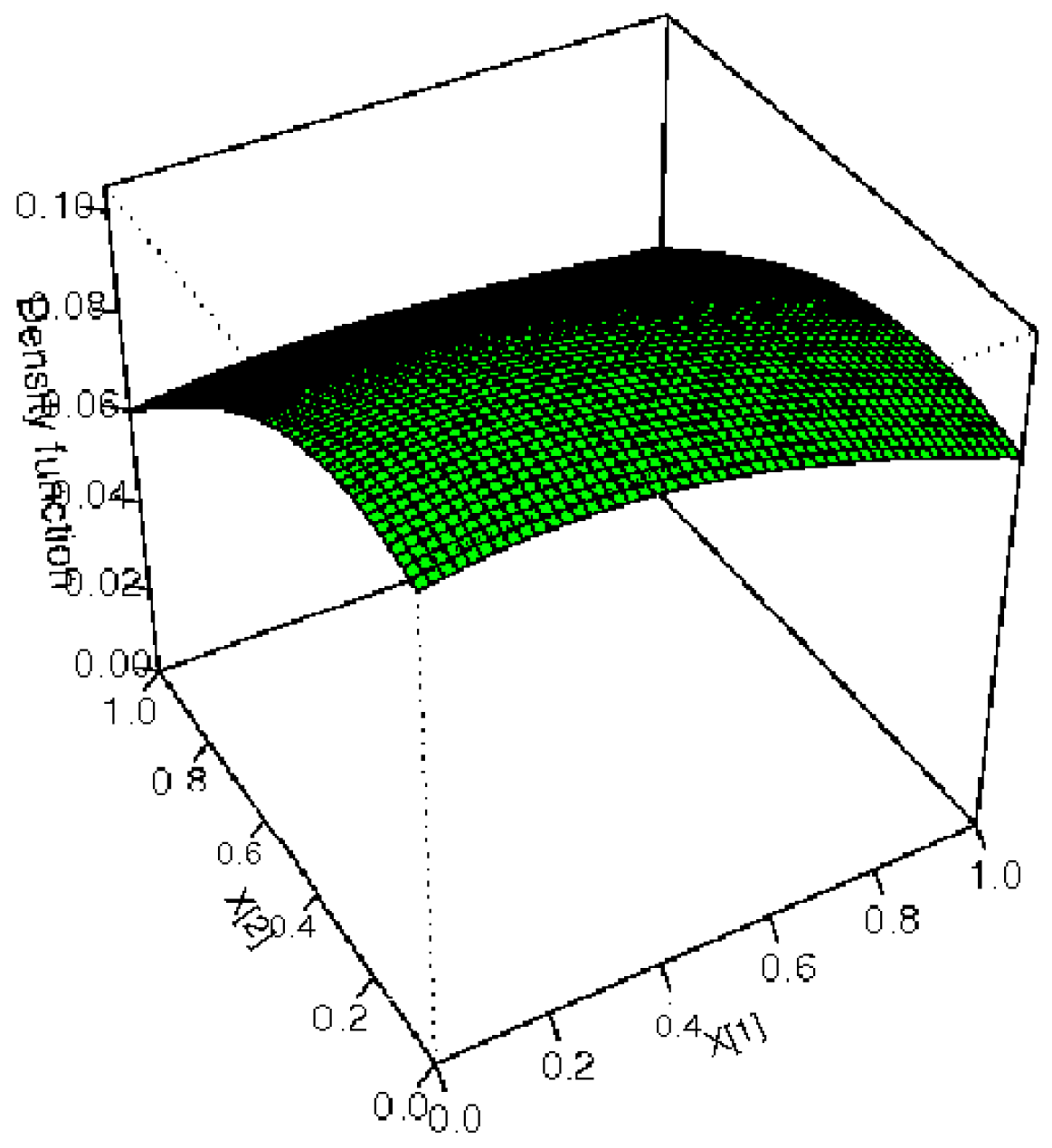
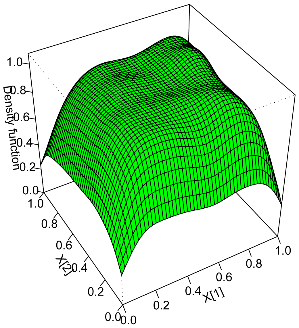
Finally, the shape of the copula in the case of real datasets in the {a1, a2} basis is also noteworthy.
Figure 4 shows that the curve reaches a quite wide plateau around 1, whereas Figure 5 shows that this plateau prevails on almost the entire [0, 1]2 set. We can therefore conclude that the theoretical analysis is indeed confirmed by the above simulation.
6.3. Conclusions
Projection pursuit is useful in evidencing characteristic structures as well as one-dimensional projections and their associated distribution in multivariate data. This article clearly demonstrates the efficiency of the φ-projection pursuit methodology for goodness-of-fit tests for copulas. Indeed, the robustness as well as the convergence results that we achieved convincingly fulfilled our expectations regarding the methodology used.


| 0. | We define g, a density with same mean and variance as f and we set g(0) = g. |
| i − 1. | We perform the goodness-of-fit test Dϕ(g(i−1), f) = 0: |
| • Should this test be passed, we derive f from | |
| And the algorithm stops. | |
| • Should this test not be verified, and should we look to approximate f, when we get to the dth iteration of the algorithm, we derive f from | |
| Otherwise, let us define a vector ai and a density g(i) by | |
| i. | Then we replace g(i−1) with g(i) and go back to i − 1. |
| 0. | We define g, a density with same mean and variance as f and we set g(0) = g. |
| i − 1. | Given , find ǎi such that the index is minimized, where fa,n is a marginal density estimate based on a⊤X1, a⊤X2,…,a⊤Xn, and where is a density estimate based on the projection to a of a Monte Carlo random sample from . |
| And we set | |
| i | Then we replace with and go back to i − 1 until the criteria reaches the stopping rule of this procedure (see below). |
| Our Algorithm | |
|---|---|
| Projection Study 0: | minimum : 0.445199 |
| at point : (1.0171,0.0055) | |
| P-Value : 0.94579 | |
| Test: | H1 : a1 ∉ 1 : True |
| Projection Study 1: | minimum : 0.009628 |
| at point : (0.0048,0.9197) | |
| P-Value : 0.99801 | |
| Test: | H0 : a2 ∈ 2 : True |
| χ2(Kernel Estimation of g(2), g(2)) | 3.57809 |
| Our Algorithm | |
|---|---|
| Projection Study 0 : | minimum : 0.057833 |
| at point : (0.9890,0.1009) | |
| P-Value : 0.955651 | |
| Test : | H1 : a1 ∉ 1 : True |
| Projection Study 1 : | minimum : 0.02611 |
| at point : (−0.1105,0.9290) | |
| P-Value : 0.921101 | |
| Test : | H0 : a2∈ 2 : True |
| χ2(Kernel Estimation of g(2), g(2)) | 1.25945 |
| Our Algorithm | |
|---|---|
| Projection Study 0: | minimum : 0.02087685 |
| at point : a1=(19.1,-12.3) | |
| P-Value : 0.748765 | |
| Test: | H0 : a1 ∈ 1 : True |
| K(Kernel Estimation of g(1), g(1) | 4.3428735 |
| Our Algorithm | |
|---|---|
| Projection Study 1: | minimum : 0.0198753 |
| at point : a2=(8.1,3.9) | |
| P-Value : 0.8743401 | |
| Test: | H0 : a2 ∈ 2 : True |
| K(Kernel Estimation of g(2), g(2)) | 4.38475324 |
| Date | Renault | Peugeot | Date | Renault | Peugeot | Date | Renault | Peugeot |
|---|---|---|---|---|---|---|---|---|
| 23/07/10 | 34.9 | 24.2 | 22/07/10 | 34.26 | 24.01 | 21/07/10 | 33.15 | 23.3 |
| 20/07/10 | 32.69 | 22.78 | 19/07/10 | 33.24 | 23.36 | 16/07/10 | 33.92 | 23.77 |
| 15/07/10 | 34.44 | 23.71 | 14/07/10 | 35.08 | 24.36 | 13/07/10 | 35.28 | 24.37 |
| 12/07/10 | 33.84 | 23.16 | 09/07/10 | 33.46 | 23.13 | 08/07/10 | 33.08 | 22.65 |
| 07/07/10 | 32.15 | 22.19 | 06/07/10 | 31.12 | 21.56 | 05/07/10 | 30.02 | 20.81 |
| 02/07/10 | 30.17 | 20.85 | 01/07/10 | 29.56 | 20.05 | 30/06/10 | 30.78 | 21.07 |
| 29/06/10 | 30.55 | 20.97 | 28/06/10 | 32.34 | 22.3 | 25/06/10 | 31.35 | 21.68 |
| 24/06/10 | 32.29 | 22.25 | 23/06/10 | 33.58 | 22.47 | 22/06/10 | 33.84 | 22.77 |
| 21/06/10 | 34.06 | 23.25 | 18/06/10 | 32.89 | 22.7 | 17/06/10 | 32.08 | 22.31 |
| 16/06/10 | 31.87 | 21.92 | 15/06/10 | 32.03 | 22.12 | 14/06/10 | 31.45 | 22.2 |
| 11/06/10 | 30.62 | 21.42 | 10/06/10 | 30.42 | 20.93 | 09/06/10 | 29.27 | 20.34 |
| 08/06/10 | 28.48 | 19.73 | 07/06/10 | 28.92 | 20.15 | 04/06/10 | 29.19 | 20.27 |
| 03/06/10 | 30.35 | 20.46 | 02/06/10 | 29.33 | 19.53 | 01/06/10 | 28.87 | 19.45 |
| 31/05/10 | 29.39 | 19.54 | 28/05/10 | 29.16 | 19.55 | 27/05/10 | 29.18 | 19.81 |
| 26/05/10 | 27.5 | 18.5 | 25/05/10 | 26.76 | 18.08 | 24/05/10 | 28.75 | 18.81 |
| 21/05/10 | 28.78 | 18.82 | 20/05/10 | 28.53 | 18.84 | 19/05/10 | 29.49 | 19.25 |
| 18/05/10 | 30.95 | 19.76 | 17/05/10 | 30.92 | 19.35 | 14/05/10 | 31.35 | 19.34 |
| 13/05/10 | 33.65 | 20.76 | 12/05/10 | 33.63 | 20.52 | 11/05/10 | 33.38 | 20.34 |
| 10/05/10 | 33.28 | 20.3 | 07/05/10 | 31 | 19.24 | 06/05/10 | 32.4 | 20.22 |
| 05/05/10 | 32.95 | 20.45 | 04/05/10 | 33.3 | 21.03 | 03/05/10 | 35.58 | 22.63 |
| 30/04/10 | 35.41 | 22.45 | 29/04/10 | 35.53 | 22.36 | 28/04/10 | 34.75 | 22.33 |
| Date | Renault | Peugeot | Date | Renault | Peugeot | Date | Renault | Peugeot |
|---|---|---|---|---|---|---|---|---|
| 27/04/10 | 36.2 | 22.9 | 26/04/10 | 37.65 | 23.73 | 23/04/10 | 36.72 | 23.5 |
| 22/04/10 | 34.36 | 22.72 | 21/04/10 | 35.01 | 22.86 | 20/04/10 | 35.62 | 22.88 |
| 19/04/10 | 34.08 | 21.77 | 16/04/10 | 34.46 | 21.71 | 15/04/10 | 35.16 | 22.22 |
| 14/04/10 | 35.1 | 22.22 | 13/04/10 | 35.28 | 22.45 | 12/04/10 | 35.17 | 21.85 |
| 09/04/10 | 35.76 | 21.9 | 08/04/10 | 35.67 | 21.67 | 07/04/10 | 36.5 | 21.89 |
| 06/04/10 | 36.87 | 22 | 01/04/10 | 35.5 | 21.97 | 31/03/10 | 34.7 | 21.8 |
| 30/03/10 | 34.8 | 22.24 | 29/03/10 | 35.7 | 22.73 | 26/03/10 | 35.54 | 22.58 |
| 25/03/10 | 35.53 | 22.73 | 24/03/10 | 33.8 | 21.82 | 23/03/10 | 34.1 | 21.58 |
| 22/03/10 | 33.73 | 21.64 | 19/03/10 | 34.12 | 21.68 | 18/03/10 | 34.44 | 21.75 |
| 17/03/10 | 34.68 | 21.98 | 16/03/10 | 34.33 | 21.88 | 15/03/10 | 33.57 | 21.53 |
| 12/03/10 | 33.9 | 21.86 | 11/03/10 | 33.27 | 21.58 | 10/03/10 | 33.12 | 21.47 |
| 09/03/10 | 32.69 | 21.54 | 08/03/10 | 32.99 | 21.66 | 05/03/10 | 32.89 | 21.85 |
| 04/03/10 | 31.64 | 21.26 | 03/03/10 | 31.65 | 20.7 | 02/03/10 | 31.05 | 20.2 |
| 01/03/10 | 30.26 | 19.54 | 26/02/10 | 30.2 | 19.39 | 25/02/10 | 29.42 | 18.98 |
| 24/02/10 | 30.9 | 19.49 | 23/02/10 | 30.54 | 19.74 | 22/02/10 | 31.89 | 20.06 |
| 19/02/10 | 32.29 | 20.67 | 18/02/10 | 32.26 | 20.41 | 17/02/10 | 31.69 | 20.31 |
| 16/02/10 | 31.08 | 19.8 | 15/02/10 | 30.25 | 19.66 | 12/02/10 | 29.56 | 19.57 |
| 11/02/10 | 31 | 20.4 | 10/02/10 | 32.78 | 21.21 | 09/02/10 | 33.31 | 22.31 |
| 08/02/10 | 32.63 | 21.95 | 05/02/10 | 32.15 | 22.33 | 04/02/10 | 33.72 | 22.86 |
| 03/02/10 | 35.32 | 23.93 | 02/02/10 | 35.29 | 23.8 | 01/02/10 | 35.31 | 24.05 |
| 29/01/10 | 34.26 | 23.64 | 28/01/10 | 33.94 | 23.31 | 27/01/10 | 33.85 | 23.88 |
| 26/01/10 | 34.97 | 24.86 | 25/01/10 | 35.06 | 24.35 | 22/01/10 | 35.7 | 24.95 |
| 21/01/10 | 36.1 | 25 | 20/01/10 | 36.92 | 25.35 | 19/01/10 | 38.4 | 25.81 |
| 18/01/10 | 39.28 | 25.95 | 15/01/10 | 38.6 | 25.7 | 14/01/10 | 39.56 | 26.67 |
| 13/01/10 | 39.49 | 26.13 | 12/01/10 | 38.36 | 25.98 | 11/01/10 | 39.21 | 26.65 |
| 08/01/10 | 39.38 | 26.5 | 07/01/10 | 39.69 | 26.7 | 06/01/10 | 39.25 | 26.32 |
| 05/01/10 | 38.31 | 24.74 | 04/01/10 | 38.2 | 24.52 |
Appendix
All the demonstrations of this article have been gathered in the Technical Report [24].
A. On the Different Families of Copula
There exists many copula families. Let us here present the most important amongst them.
A.1. Elliptical Copulas
The Gaussian Copula
The Gaussian copula can be used in several fields. For example, many credit models are built from this copula, which also presents the property to make extreme values (minimal or maximal) independent in the limit; see Joe [2] for more details. For example, in ℝ2, it is derived from the bivariate normal distribution and from Sklar's theorem. Defining Ψρ as the standard bivariate normal cumulative distribution function with ρ correlation, the Gaussian copula function is Cρ(u, v) = Ψρ (Ψ−1(u), Ψ−1(v)) where u, v ∈ [0, 1] and where Ψ is the standard normal cumulative distribution function. Then, the copula density function is :
The Elliptical Copula
Let us begin with defining the class of elliptical distributions and its properties—see also Cambanis [17], Landsman [18]:
Definition A.1
X is said to abide by a multivariate elliptical distribution, denoted X ∼ Ed(μ, Σ, ξd), if X has the following density, for any x in ℝd:
where ξd is referred as the “density generator”,
where αd is a normalisation constant, such that ,
with .
Property A.1
(1) For any X ∼ Ed(μ, Σ, ξd), for any m × d matrix with rank m ≤ d, A, and for any m-dimensional vector b, we have AX + b ∼ Em(Aμ + b, AΣA′, ξm).
Therefore, any marginal density of multivariate elliptical distribution is elliptical, i.e., , 1 ≤ i ≤ d, with . (2) Corollary 5 of Cambanis [17] states that conditional densities with elliptical distributions are also elliptical. Indeed, if X = (X1, X2)′ ∼ Ed(μ, Σ, ξd), with X1 (resp. X2) of size d1 < d (resp. d2 < d), then X1/(X2 = a) ∼ Ed1(μ′, Σ′, ξd1) with and , with μ = (μ1, μ2) and Σ = (Σij)1≤i,j≤2.
Remark A.1
Landsman [18] shows that multivariate Gaussian distributions derive from ξd(x) = e−x and that if X = (X1, …, Xd) has an elliptical density such that its marginals verify E(Xi) < ∞ and for 1 ≤ i ≤ d, then μ is the mean of X and Σ is a multiple of the covariance matrix of X. Consequently, from now on, we will assume this is indeed the case.
Definition A.2
Let t be an elliptical density on ℝk and let q be an elliptical density on ℝk′. The elliptical densities t and q are said to belong to the same family of elliptical densities, if their generating densities are ξk and ξk′ respectively, which belong to a common given family of densities.
Example A.1
Consider two Gaussian densities
 (0, 1) and
((0, 0), Id2). They are said to belong to the same elliptical family as they both present x ↦ e−x as generating density.
(0, 1) and
((0, 0), Id2). They are said to belong to the same elliptical family as they both present x ↦ e−x as generating density.
Finally, let us introduce the definition of an elliptical copula which generalizes the above overview of the Gaussian copula:
Definition A.3
Elliptical copulas are the copulas of elliptical distributions.
A.2. Archimedean Copulas
These copulas exhibit a simple form as well as properties such as associativity. They also present a variety of dependent structures. They can generally be defined under the following form
Let us now present several examples:
Clayton copula:
The Clayton copula is an asymmetric Archimedean copula, displaying greater dependency in the negative tail than in the positive tail. Let us define X (resp. Y) as the random vector having F (resp G) as cumulative distribution function (CDF). Assuming that the vector (X, Y) has a Clayton copula, then this copula is given by:
And its generator is:
For θ = 0, the random variables are independent.
Gumbel copula:
The Gumbel copula (Gumbel-Hougard copula) is an asymmetric Archimedean copula, presenting greater dependency in the positive tail than in the negative tail. This copula is given by:
Frank copula:
The Frank copula is a symmetric Archimedean copula given by:
A.3. Periodic Copula
In 2005, Alfonsi and Brigo [25] derived a new way of generating copulas based on periodic functions. Defining h (resp.
 ) as a 1-periodic non-negative function that integrates to 1 over [0, 1] (resp. as a double primitive of h), then both
B. ϕ-Divergence
Let us call ha the density of a⊤Z if h is the density of Z. Let φ be a strictly convex function defined by , and such that φ(1) = 0.
Definition B.1
We define a ϕ-divergence of P from Q, where P and Q are two probability distributions over a space Ω such that Q is absolutely continuous with respect to P, by
The most used distances (Kullback, Hellinger or χ2) belong to the Cressie-Read family (see Cressie-Read [26], Csiszár I. [27] and the books of Friedrich and Igor [28], Pardo Leandro [29] and Zografos K. [30]). They are defined by a specific φ. Indeed,
- -
with the Kullback-Leibler divergence, we associate φ(x) = K(x) = xln(x) − x + 1
- -
with the Hellinger distance, we associate
- -
with the χ2 distance, we associate
- -
more generally, with power divergences, we associate , where γ ∈ ℝ \ (0, 1)
- -
and, finally, with the L1 norm, which is also a divergence, we associate φ(x) = |x − 1|.
Let us now expose some well-known properties of divergences.
Property B.1
We have Dϕ(P, Q) = 0 ⇔ P = Q.
Property B.2
The divergence function Q ↦ Dϕ(Q, P) is convex and lower semi-continuous for the topology that makes all the applications of the form Q ↦ ∫ fdQ continuous (where f is bounded and continuous), and lower semi-continuous for the topology of the uniform convergence.
Finally, we will also use the following property derived from the first part of corollary (1.29) page 19 of Friedrich and Igor [28],
Property B.3
If T : (X, A) → (Y, B) is measurable and if Dϕ(P, Q) < ∞, then Dϕ(P, Q) ≥ Dϕ(PT−1, QT−1) with equality being reached when T is surjective for (P, Q).
C. Miscellaneous
Lemma C.1
For any p ≤ d, we have .
Lemma C.2
We have .
Lemma C3
Should there exist a family (ai)i=1…d such that , with j < d, with f, n and h being densities, then this family is an orthogonal basis of ℝd.
Lemma C.4
is reached when the ϕ-divergence is greater than the L1 distance as well as the L2 distance.
Lemma C.5
Whenever there exists p, p ≤ d, such that Dϕ(g(p), f) = 0, then the family of (ai)i=1,…,p is free and is orthogonal.
Lemma C.6
For any continuous density f, we have .
D. Study of the Sample
Let X1, X2,‥,Xm be a sequence of independent random vectors with the same density f. Let Y1, Y2,‥,Ym be a sequence of independent random vectors with the same density g. Then, the kernel estimators fm, gm, fa,m and ga,m of f, g, fa and ga, for all , almost surely and uniformly converge since we assume that the bandwidth hm of these estimators meets the following conditions (see Bosq [32]):
Let us consider
Our objective is to estimate the minimum of . To achieve this, samples have to be truncated:
Let us consider now a positive sequence θm such that θm → 0, , where ym is the almost sure convergence rate of the kernel density estimator— , see lemma C.6— , where is defined by
We then generate fm, gm and gb,m from the starting sample and we select the Xi and Yi vectors such that fm(Xi) ≥ θm and gb,m(b⊤Yi) ≥ θm, for all i and for all .
The vectors meeting these conditions will be called X1, X2, …, Xn and Y1, Y2, …, Yn.
Consequently, the next proposition provides us with the condition required to derive our estimates:
Proposition D.1
Using the notations introduced in Broniatowski [33] and in Section 4.1, it holds .
Remark D.1
With the Kullback-Leibler divergence, we can take for θm the expression m−ν, with .
E. Hypotheses' Discussion
Not all hypotheses will be used simultaneously.
Hypotheses (A1) and (A4) lead us to assume we deal with a saddle point: being used to demonstrate the convergence of čn(a) and γk towards ak, they make it easier to use the dual form of the divergence. Moreover, since our criteria is differentiable on and continuously differentiable on ℝd, these hypotheses can be easily obtained. However, if other discontinuities, for which the criteria can not be extended by continuity, do exist, then the above hypotheses would be very difficult to verify even in very favorable cases.
As shown by the below subsection for relative entropy, hypothesis (A2) generally holds.
Hypotheses (A5) and (A7) are classical hypotheses from which a limit distribution for the criteria can be derived. Yet these hypotheses are difficult to obtain when the criteria admits discontinuities—close to the co-vectors of f—for which it can not be continuously differentiable.
Hypothesis (A6) thus enables to create a stopping rule for the process since this hypothesis is equivalent to the nullity of the application in ak.
Hypothesis (A0) constitutes an alternative to the starting hypothesis according to which the divergence should be greater than the L1 distance. Although weaker, this hypothesis also requires that for all i, we have K (g(i), f) ≥ ∫ |f(x) − g(i)(x)|dx at each iteration of the algorithm.
E.1. Discussion of (A2)
Let us work with the Kullback-Leibler divergence and with g and a1.
For all , we have , since, for any b in , the function is a density. The complement of ΘDϕ in is ∅ and then the supremum looked for in ℝ̅ is −∞. We can therefore conclude. It is interesting to note that we obtain the same verification with f, g(k−1) and ak.
E.2. Discussion of (A3)
This hypothesis consists in the following assumptions:
(0) We work with the Kullback-Leibler divergence,
(1) We have , i.e., —we could also derive the same proof with f, g(k−1) and ak
Preliminary (A)
Shows that through a reductio ad absurdum, i.e., if we assume A ≠ ∅.
Thus, our hypothesis enables us to derive
Preliminary (B)
Shows that through a reductio ad absurdum, i.e., if we assume B ≠ ∅.
Thus, our hypothesis enables us to derive
We can consequently conclude as above.
Let us now verify (A3):
We have . Moreover, the logarithm ln is negative on and is positive on .
Thus, the preliminary studies (A) and (B) show that and always present a negative product. We can therefore conclude, since (c, a) ↦ PM(c, a1) − PM(c, a) is not null for all c and for all a, with a ≠ a1.
References
- Sklar, M. Fonctions de répartition à n dimensions et leurs marges. Publ. Inst. Stat. Univ. 1959, 8, 229–231. [Google Scholar]
- Joe, H. Multivariate Models and Dependence Concepts. Monographs on Statistics and Applied Probability, 1st ed.; Chapman and Hall/CRC: London, UK, 1997. [Google Scholar]
- Nelsen, R.B. An introduction to Copulas. Springer Series in Statistics, 2nd ed.; Springer: New York, NY, USA, 2006. [Google Scholar]
- Carriere, J.F. A large sample test for one-parameter families of Copulas. Comm. Stat. Theor. Meth. 1994, 23, 1311–1317. [Google Scholar]
- Genest, C.; Rémillard, B. Tests of independence and randomness based on the empirical Copula process. Test 2004, 13, 335–370. [Google Scholar]
- Fermanian, J.D. Goodness of fit tests for copulas. J. Multivariate Anal. 2005, 95, 119–152. [Google Scholar]
- Genest, C.; Quessy, J.F.; Rémillard, B. Goodness-of-fit procedures for copula models based on the probability integral transformation. Scand. J. Stat. 2006, 33, 337–366. [Google Scholar]
- Michiels, F.; De Schepper, A. A Copula Test Space Model—How to Avoid the Wrong Copula Choice. Kybernetika 2008, 44, 864–878. [Google Scholar]
- Genest, C. Metaelliptical copulas and their use in frequency analysis of multivariate hydrological data. Water Resour. Res. 2009, 43, W09401:1–W09401:12. [Google Scholar]
- Mesfioui, M.; Quessy, J.F.; Toupin, M.H. On a new goodness-of-fit process for families of copulas. La Revue Canadienne de Statistique 2009, 37, 80–101. [Google Scholar]
- Genest, C.; Rémillard, B. Goodness-of-fit tests for copulas: A review and a power study. Insurance: Math. Econ. 2009, 44, 199–213. [Google Scholar]
- Berg, D. Copula goodness-of-fit testing: An overview and power comparison. Eur. J. Finance 2009, 15, 675–701. [Google Scholar]
- Bücher, A.; Dette, H. Some comments on goodness-of-fit tests for the parametric form of the copula based on L2-distances. J. Multivar. Anal. 2010, 101, 749–763. [Google Scholar]
- Broniatowski, M.; Leorato, S. An estimation method for the Neyman chi-square divergence with application to test of hypotheses. J. Multivar. Anal. 2006, 97, 1409–1436. [Google Scholar]
- Friedman, J.H.; Stuetzle, W.; Schroeder, A. Projection pursuit density estimation. J. Am. Statist. Assoc. 1984, 79, 599–608. [Google Scholar]
- Huber, P.J. Projection pursuit. Ann. Stat. 1985, 13, 435–525. [Google Scholar]
- Cambanis, S.; Huang, S.; Simons, G. On the theory of elliptically contoured distributions. J. Multivar. Anal. 1981, 11, 368–385. [Google Scholar]
- Landsman, Z.M.; Valdez, E.A. Tail conditional expectations for elliptical distributions. N. Am. Actuar. J. 2003, 7, 55–71. [Google Scholar]
- Yohai, V.J. Optimal robust estimates using the Kullback-Leibler divergence. Stat. Probab. Lett. 2008, 78, 1811–1816. [Google Scholar]
- Toma, A. Optimal robust M-estimators using divergences. Stat. Probab. Lett. 2009, 79, 1–5. [Google Scholar]
- Huber, P.J. Robust Statistics; Wiley: New York, NY, USA, 1981; (republished in paperback, 2004). [Google Scholar]
- van der Vaart, A.W. Asymptotic statistics. Cambridge Series in Statistical and Probabilistic Mathematics; Cambridge University Press: Cambridge, UK, 1998. [Google Scholar]
- Scott, D.W. Multivariate Density Estimation. Theory, Practice, and Visualization. Wiley Series in Probability and Mathematical Statistics: Applied Probability and Statistics; A Wiley-Interscience Publication. John Wiley and Sons, Inc.: New York, NY, USA, 1992. [Google Scholar]
- Touboul, J. Goodness-of-fit Tests For Elliptical And Independent Copulas Through Projection Pursuit. arXiv. Statistics Theory 2011. arXiv: 1103.0498. [Google Scholar]
- Aurélien, A.; Damiano, B. New families of Copulas based on periodic functions. Commun. Stat. Theor. Meth. 2005, 34, 1437–1447. [Google Scholar]
- Cressie, N.; Read, T.R.C. Multinomial goodness-of-fit tests. J. R. Stat. Soc. Series B 1984, 46, 440–464. [Google Scholar]
- Csiszár, I. On topology properties of f-divergences. Studia Sci. Math. Hungar. 1967, 2, 329–339. [Google Scholar]
- Liese, F.; Vajda, I. Convex Statistical Distances; BSB B. G. Teubner Verlagsgesellschaft: Leipzig, Germany, 1987. [Google Scholar]
- Pardo, L. Statistical Inference Based on Divergence Measures. Statistics: Textbooks and Monographs; Chapman & Hall/CRC: Boca Raton, FL, USA, 2006. [Google Scholar]
- Zografos, K.; Ferentinos, K.; Papaioannou, T. φ-divergence statistics: sampling properties and multinomial goodness of fit and divergence tests. Commun. Stat. Theor. Meth. 1990, 19, 1785–1802. [Google Scholar]
- Azé, D. Eléments D'analyse Convexe et Variationnelle, Ellipses; Dunod: Paris, French, 1997. [Google Scholar]
- Bosq, D.; Lecoutre, J.P. Livre-Theorie De L'Estimation Fonctionnelle; Economica, 1999. [Google Scholar]
- Broniatowski, M.; Keziou, A. Parametric estimation and tests through divergences and the duality technique. J. Multivar. Anal. 2009, 100, 16–36. [Google Scholar]
- Black and Scholes. The pricing of options and corporate liabilities. J. Polit. Econ. 1973, 81, 635–654. [Google Scholar]
- Classification: MSC 62H05 62H15 62H40 62G15
© 2011 by the author; licensee MDPI, Basel, Switzerland. This article is an open access article distributed under the terms and conditions of the Creative Commons Attribution license (http://creativecommons.org/licenses/by/3.0/.)
Share and Cite
Touboul, J. Goodness-of-Fit Tests For Elliptical and Independent Copulas through Projection Pursuit. Algorithms 2011, 4, 87-114. https://doi.org/10.3390/a4020087
Touboul J. Goodness-of-Fit Tests For Elliptical and Independent Copulas through Projection Pursuit. Algorithms. 2011; 4(2):87-114. https://doi.org/10.3390/a4020087
Chicago/Turabian StyleTouboul, Jacques. 2011. "Goodness-of-Fit Tests For Elliptical and Independent Copulas through Projection Pursuit" Algorithms 4, no. 2: 87-114. https://doi.org/10.3390/a4020087