A Novel Algorithm for Macromolecular Epitope Matching

Abstract

Many macromolecules, namely proteins, show functional substructures or epitopes defined by characteristic spatial arrangements of groups of specific atoms or residues. The identification of such substructures in a set of macromolecular 3D-structures solves an important problem in molecular biology as it allows the assignment of functions to molecular moieties and thus opens the possibility of a mechanistic understanding of molecular function. We have devised an algorithm that models a functional epitope formed by a group of atoms or residues as set of points in cartesian space with associated functional properties. The algorithm searches for similar epitopes in a database of structures by an efficient multi-stage comparison of distance sets in the epitope and in the structures from the database. The search results in a list of optimal matches and corresponding optimal superpositions of query epitope and matching epitopes from the database. The algorithm is discussed against the background of related approaches, and it is successfully tested in three application scenarios: global match of two homologous proteins, search for an epitope on a homologous protein, and finding matching epitopes in a protein database.

1. Introduction

Biological macromolecules usually have specific three-dimensional sub-structures that allow them to exert their special functions (henceforth we will call these three-dimensional sub-structures “epitopes”, a term that originally had been used for sub-structures recognized by antibodies). For instance, enzymes have binding pockets that fit the three-dimensional structures of their substrates or co-factors, proteins in signal transduction have characteristic surface patches fitting those of binding partners along the respective signal cascade, strands of DNA hybridize with structurally complementary strands, etc. Evolution has re-used many of these functions, and, consequently, we find the same or similar epitopes packed into different molecules. This fact can be exploited to address central problems in molecular biology; e.g. it is possible to use structurally characterized epitopes of known function on a certain molecular three-dimensional structure to search for similar epitopes on other molecules and in this way elucidate the function of the latter molecules. The quickly growing number of structures in the Protein Data Bank [1] and other molecular databases opens the possibility for this type of studies, but it also necessitates efficient search algorithms for finding similar epitopes. Another application that is of particular interest to us lies in protein engineering where the goal is to mutate proteins in such a way that they carry a particular functional epitope; in this case an algorithm for epitope matching and comparison can be used in a procedure for optimizing proteins by finding the best mutants [2].

These algorithms should solve a matching problem that can be described as finding sets of atoms in the database that, after optimal superposition, closely match the coordinates of atoms in the epitope, with each matching pair of atoms being of the same type. For instance, we may search for an epitope given by four atoms, namely three oxygen atoms in carboxylate groups with Cartesian coordinates o₁, o₂, o₃, respectively, and a calcium ion with Cartesian coordinates $\mathbf{ca}$. In this case we have solved the matching problem if we identify in a database of molecular three-dimensional structures one or several sub-structures of three carboxylate-oxygens and a calcium ion with Cartesian coordinates O₁, O₂, O₃ and Ca, respectively, so that the root-mean-square-deviation (RMSD) R between the groups is minimal, i.e. $R=\sqrt{\frac{1}{4}\left({\left(\mathbf{Ca}-\mathbf{ca}\right)}^2+{\sum }_{i=1}^3{\left({\mathbf{O}}_i-{\mathbf{o}}_i\right)}^2\right)}\stackrel{!}{=}min$. It is noteworthy that there are three atoms of the same type (oxygen) in both sets. This means that the matching problem has two aspects: one has to find not only a matching set of atoms but also the permutation that leads to the minimal R. Further, it should be noted that we imply a simple model that is frequently used in which molecules are sets of point-like atoms, or pseudo-atoms representing building-blocks such as amino-acids in proteins; each atom or pseudo-atom is given by its Cartesian coordinates and a nominal type descriptor.

Several approaches have been applied to the solution of this and related 3D-matching problems (for reviews see e.g. Ref. [3,4]). For the important macromolecular class of proteins, several efficient matching algorithms such as Dali [5] or Ssap [6] have been devised that make explicit use of special properties of proteins as the sequential and spatial arrangement of their secondary structures and that therefore are very fast. More generally applicable is the geometric hashing approach: one first prepares a large hash table encoding all structures in the database, then the query is very efficiently compared to the entries of the table [7]. The matching problem can be formulated elegantly in terms of graph theory with vertices corresponding to (pseudo-)atoms and edges corresponding to Cartesian distances or chemical bonds. Consequently, many algorithms have been invented to solve the matching problem in the form of a search for isomorphic subgraphs, especially maximum common subgraphs (MCS) of two graphs (for review see [8]); a well-known member of this family is the algorithm by Ullmann [15] that has been adapted for molecular matching problems in Assam [9]. The Ullmann algorithm represents the graphs to be matched by adjacency matrices with elements 1 symbolizing neighborhood and 0 otherwise. The matching could then be carried out by brute-force comparison; however, Ullmann reduces the search space by a refinement procedure that early on eliminates 1-elements that violate conditions that have to be fulfilled by isomorphic graphs.

We propose an approach for the solution of the matching problem that does not take into account the sequential nature or secondary structures of proteins. Instead, our EpitopeMatch algorithm identifies epitopes that are similar to a query epitope comprising an arbitrary set of atoms given by their types and Cartesian coordinates. The algorithm thus is applicable to general macromolecules without adaptation. Further, the proposed algorithm is a one-pass method that operates directly on the macromolecular structure sets, e.g. in the form of the widely used files from the Protein Data Bank without preparatory steps. This feature is important for us since we apply the method also in the process of protein engineering for on-the-fly comparisons of many novel structures generated in silico. In terms of graph theory our method is a heuristic to identify common, connected, approximately maximal subgraphs of two graphs. Unlike the Ullmann algorithm EpitopeMatch does not operate on adjacency matrices but first tries to find small and accurately matching subgraphs and then iteratively extends and joins these matches to larger and less accurately matching subgraphs. The iterative nature makes EpitopeMatch superficially similar to the Maxsubalgorithm [10], though the latter algorithm has been formulated for chemical 2D-graphs. Although EpitopeMatch makes use of cliques, it does not aim at finding all cliques as e.g. the Bron-Kerbosch algorithm [11]. Two of the features of EpitopeMatch that we have not seen in other algorithms is, firstly, a probability-like score for each pair of matching atoms indicating the certainty of this match, and, secondly, the generation of a Pareto-optimal set of matches in terms of the objective dimensions number of matching pairs and RMSD. In the following we will characterize the problem to be solved more quantitatively, describe the EpitopeMatch algorithm, and present non-trivial applications on proteins.

2. Results and Discussion

2.1. Description of problem and assessment of problem size

We are looking for matches between the query set of atomic Cartesian coordinates ${\mathbf{x}}_i,i=1,\dots ,m$ and atom types $s_i$, with corresponding structures in a database of three-dimensional molecular structures numbered $j=1,\dots ,N$, where the jth molecular structure in the database has atomic Cartesian coordinates ${\mathbf{y}}_{jk},k=1,\dots ,n_j$ and atom types $t_{jk}$. The number τ of atom types is limited, e.g. “atoms” may be centers of amino-acid residues of 20 types, or real atoms with types corresponding to chemical elements, or atoms with certain property types (charged, polar, neutral, etc.).

A full match, or, for brevity, a match of the query in molecule j is defined as an assignment of all m coordinates ${\mathbf{x}}_i$ of the query to m coordinates ${\mathbf{y}}_{ji}$ of molecule j so that $\forall i\in \{1,\dots ,m\}:s_i=t_{ji}$ (if needed the $t_i$ are renumbered). It is possible that several matches exist in the same molecule and it is likely that many matches can be found in the database. An optimal match is defined as a match for which the RMSD $R=\sqrt{\frac{1}{m}{\sum }_{i=1}^m{\left({\mathbf{x}}_i-{\mathbf{y}}_{ji}\right)}^2}$ is minimal. We are interested mainly in optimal or near-optimal matches because in these cases the physico-chemical properties of the query and the matching epitope promise to be similar.

For the estimation of the problem complexity it is realistic to assume that the number of atoms $q_i$ of any type $i=1,\dots ,\tau$ in the query is smaller than the number of atoms $M_i$ of the corresponding types $i=1,\dots ,\tau$, since epitopes typically contain much less atoms than the molecules in the database. The theoretical number Θ of matches of a query in a database of N molecules is then

$$\Theta =\sum _{j=1}^N\prod _{i=1}^{\tau }\frac{M_{ji}!}{(M_{ji}-q_i)!}.$$

(1)

To assess a realistic size of Θ we take the medium sized protein molecule human hemoglobin as a database representative. As atoms we use $C_{\alpha }$ atoms, and atoms may have one type out of $\tau =4$, namely hydrophobic, polar, positive, or negative, depending on electric charge and solubility in water. As an example for a query epitope we use the heme binding pocket, also in human hemoglobin, formed by 16 residues, including $q_1=12$ hydrophobic, $q_2=3$ polar, $q_3=1$ positive, and $q_4=0$ negative residues. Since it is known that there are four similar heme binding pockets in hemoglobin, the search for optimal and near-optimal matches with the query pocket should result in four matches. The whole human hemoglobin molecule contains 574 amino acid residues, including $M_1=276$ hydrophobic, $M_2=188$ polar, $M_3=56$ positive, and $M_4=54$ negative residues. The product in Equation 1 then amounts to about ${10}^{38}$, which means that taking into account the structure of human hemoglobin alone, the four optimal and near-optimal matches form a minute fraction of all theoretical matches. Moreover, with the number N of relevant molecules in the Protein Data Bank being of the order of ${10}^4$, we have $\Theta \approx {10}^{42}$. This number makes it clear that a complete enumeration of all possible matches in search for optimal matches is not feasible. We therefore have devised the following EpitopeMatch algorithm.

2.2. Algorithm

Rationale

The core of the problem is to find a match of a query atom set A in a larger atom set B, where $A=\left\{a_1,\dots ,a_m\right\}$ with each atom $a_i=\left({\mathbf{x}}_i,s_i\right)$ given by its Cartesian co-ordinates ${\mathbf{x}}_i$ and atom type $s_i$, and analogously $B=\left\{b_1,\dots ,b_n\right\}$ with $b_j=\left({\mathbf{y}}_j,t_j\right)$. In the language of graph theory, the distance matrix $D_A$ of A defines a complete graph on A with nodes standing for atoms and being attributed by atom types $s_i$ and edges standing for distances $\left|{\mathbf{x}}_i-{\mathbf{x}}_j\right|$ between atoms. The distance matrix $D_B$ defines a complete graph on B in an analogous way with nodes attributed by types $t_i$ and edges by distances $\left|{\mathbf{y}}_i-{\mathbf{y}}_j\right|$. In the following we use the terms “atom”, “node”, and “vertex” synonymously. To keep the presentation simple, we assume that all atoms are of the same type, i.e. $s_i=t_j\forall i,j:i\in \left\{1,\dots ,m\right\},j\in \left\{1,\dots ,n\right\}$; the actual implementation of the algorithm does not have this restriction, as shown in the applications section.

The essential assumption underlying EpitopeMatchis that the query epitope and its cognate optimal matches differ not too much, i.e. if $a_i$ is matched with $b_k$ and $a_j$ with $b_l$, then the distance difference $d_{ijkl}=\left|\left|{\mathbf{x}}_i-{\mathbf{x}}_j\right|-\left|{\mathbf{y}}_k-{\mathbf{y}}_l\right|\right|$ should be small. The assumption is justified by the purpose for which EpitopeMatch has been developed, namely to identify patterns that as a whole have similar physico-chemical properties. This similarity crucially relies on the similar geometric arrangement of the corresponding functional groups in the matched sets. The exploitation of the assumption has two consequences: firstly, most of the potentially existing matches are not taken into account because they are too different and thus the search space is drastically reduced, and, secondly, the RMSD values R between the corresponding sets of coordinates in optimal matches are small, typically up to a few Å.

The assumption is exploited in the following way. EpitopeMatchstarts by identifying small and accurate (low $d_{ijkl}$) subgraph matches by explicitly considering only $d_{ijkl}<\delta$ with a low threshold δ of typically $\delta \approx 0.1$ Å. Then the algorithm iteratively increases δ and extends previously found subgraph matches, and, if possible, joins them to larger subgraph matches. The iteration is stopped when δ exceeds a preset limit, or when a full match with the query set A has been achieved. This central part of the algorithm – the finding of an optimal structural alignment with the query – is shown as pseudo-code in Algorithm 1 (see Appendix).

After the iteration in Algorithm 1 with increasing ${\delta }_1$, the best matching sets are optimally superimposed in Cartesian space and the respective R values are computed. Finally, if the algorithm scans a whole database of structures $B_i$, it generates a Pareto-optimal set with respect to the objective dimensions RMSD R and number of matching pairs $N_p$.

The algorithm is organized in the five steps described below.

Step 1: Finding seed matches with small distance tolerance

We set the initial distance tolerance ${\delta }_1$ to a small value that roughly corresponds to the accuracy of the experimental method used for determination of the macromolecular structure, e.g. ${\delta }_1=$0.1 Å. As seeds of possible matches we try to identify pairs of atoms $a_i$ and $b_k$ from A and B, respectively, for which there are at least ν other atoms $a_j$ and $b_l$, respectively, with distances $\left|{\mathbf{x}}_i-{\mathbf{x}}_j\right|$ and $\left|{\mathbf{y}}_k-{\mathbf{y}}_l\right|$ differing by at most ${\delta }_1$. To this end we compare $D_A$ with $D_B$ element by element:

$$d_{ijkl}=\left|D_{A,ij}-D_{B,kl}\right|\le {\delta }_1.$$

(2)

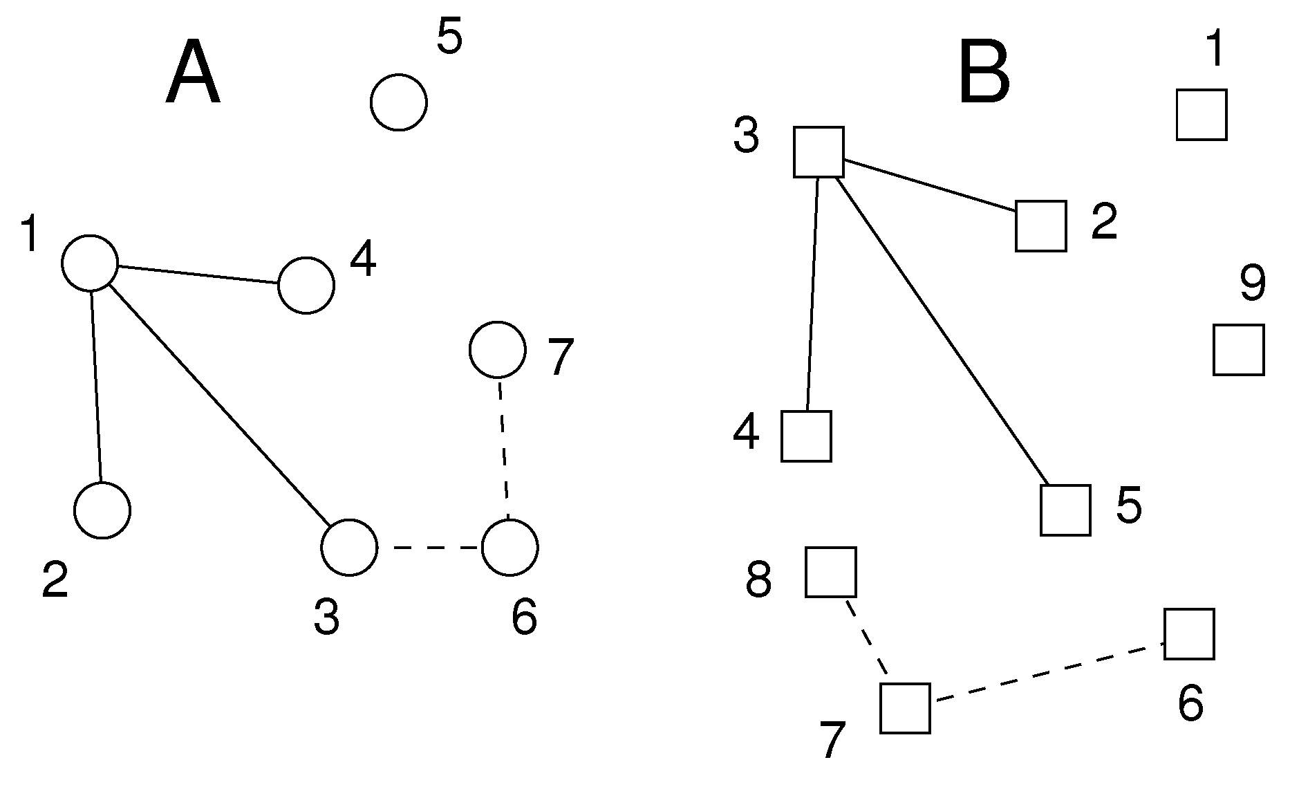
The parameter ν is set by the user. We have obtained good results with $\nu =4$. The resulting pairs of atoms $ab$ define pairs of star graphs of at least ν edges, as shown schematically in Figure 1.

The time complexity in this step is $O\left(m^2{n}^2\right)$, since it is dominated by the number of distance difference computations given by $\frac{1}{4}m·(m-1)·n·(n-1)$, i.e. the number of pairs of matrix elements in the upper diagonal parts of the symmetric distance matrices $D_A$ and $D_B$ (see Algorithm 2 in Appendix). This step determines the overall time complexity of EpitopeMatch. In the current implementation of the algorithm we reduce time complexity by several means, e.g. by avoiding to investigate distance differences with distances in B beyond the largest distance in the query epitope A.

In general some seed matches can be consolidated after investigation of further distance differences between nodes in the stars, whereas many other seed matches turn out to be dead ends – a kind of noise of accidental false positive matches. Step 2 is intended to reduce this noise.

Figure 1. Schematic of situation after Step 1 of algorithm. The two sets A and B of atoms to be matched are shown as circles and squares, respectively. For clarity, all atoms are of the same type, and the minimum degree of the central node in each star is $\nu =2$. We find two pairs of atoms from A and B with $\nu =2$ or more distance differences smaller than ${\delta }_1$: atom pair $a_1{b}_3$ (solid lines) and atom pair $a_6{b}_7$ (dotted lines). For instance $a_1{b}_3$ has three distance differences smaller than ${\delta }_1$, namely $\left|\left|{\mathbf{x}}_1-{\mathbf{x}}_2\right|-\left|{\mathbf{y}}_3-{\mathbf{y}}_4\right|\right|$, $\left|\left|{\mathbf{x}}_1-{\mathbf{x}}_3\right|-\left|{\mathbf{y}}_3-{\mathbf{y}}_5\right|\right|$, $\left|\left|{\mathbf{x}}_1-{\mathbf{x}}_4\right|-\left|{\mathbf{y}}_3-{\mathbf{y}}_2\right|\right|$.

Figure 1. Schematic of situation after Step 1 of algorithm. The two sets A and B of atoms to be matched are shown as circles and squares, respectively. For clarity, all atoms are of the same type, and the minimum degree of the central node in each star is $\nu =2$. We find two pairs of atoms from A and B with $\nu =2$ or more distance differences smaller than ${\delta }_1$: atom pair $a_1{b}_3$ (solid lines) and atom pair $a_6{b}_7$ (dotted lines). For instance $a_1{b}_3$ has three distance differences smaller than ${\delta }_1$, namely $\left|\left|{\mathbf{x}}_1-{\mathbf{x}}_2\right|-\left|{\mathbf{y}}_3-{\mathbf{y}}_4\right|\right|$, $\left|\left|{\mathbf{x}}_1-{\mathbf{x}}_3\right|-\left|{\mathbf{y}}_3-{\mathbf{y}}_5\right|\right|$, $\left|\left|{\mathbf{x}}_1-{\mathbf{x}}_4\right|-\left|{\mathbf{y}}_3-{\mathbf{y}}_2\right|\right|$.

Step 2: Consolidation of matching stars to cliques

The aim of this step is to identify amongst the matching stars obtained from Step 1 those matches that are guaranteed to have between all corresponding nodes a maximum distance difference below a second distance tolerance ${\delta }_2\ge {\delta }_1$. This is achieved by testing all distance differences between corresponding nodes in the graphs from Step 1 that have not been investigated in the previous steps for fulfillment of Inequality 3 (see also Figure 2):

$$\left|D_{A,ij}-D_{B,kl}\right|\le {\delta }_2.$$

(3)

The exact relation between ${\delta }_1$ and ${\delta }_2$ is defined by the user and determines how sensitive and specific the algorithm finally is. We have found ${\delta }_2=4·{\delta }_1$ to give reasonable results for various protein matching problems.

In this way, the nodes in the stars from Step 1 are supplemented with new edges. The aim is now to consolidate these graphs to complete graphs (cliques) with all edges fulfilling Inequality 3. To this end, every pair of nodes $a_i{b}_k$ is attributed with its degree, i.e. the number of edge pairs that fulfill Inequality 3. Then the node pair with the smallest degree is removed from the graph and the degrees in the graph are recomputed; this is repeated until all remaining nodes have the same degree. (We have found that the removal of weak nodes is more specific if we use as criterion the sum of degrees of the node and of its neighbors, instead of using the degree of the node alone.) If the number of nodes drops below ν the graph is abandoned. The remaining graphs then form cliques of at least ν members (Figure 2, and pseudo-code in Algorithm 3 in Appendix).

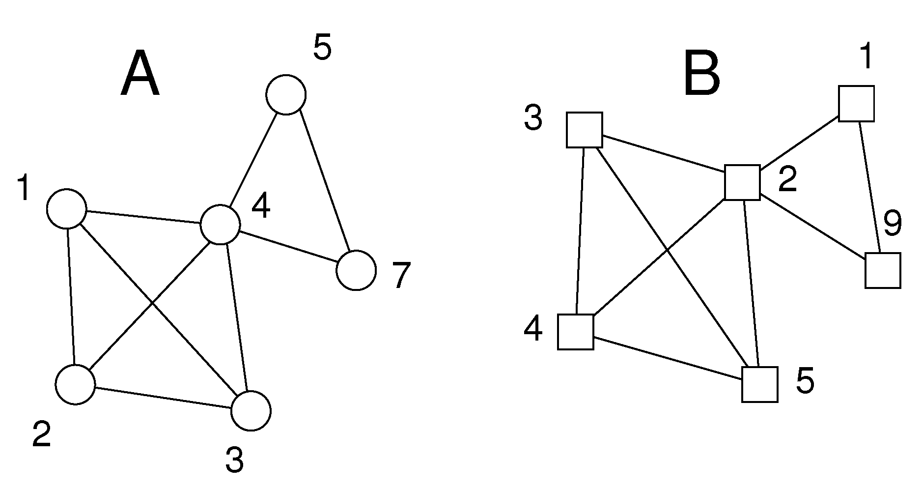
Figure 2. Schematic of situation in Step 2 after identification of matching cliques. The distance differences not yet investigated in the previous step are tested for fulfillment of inequality 3. Here, these are $\left|D_{A,23}-D_{B,45}\right|$, $\left|D_{A,34}-D_{B,52}\right|$, $\left|D_{A,24}-D_{B,42}\right|$, the differences of the lengths of the corresponding bold edges. After having passed this test it is guaranteed that all corresponding edges of the two complete graphs (cliques) have distance differences of ${\delta }_2$ or less. The stars around $a_6$ and $b_7$ in Figure 1 have not passed the test and have been dropped.

Figure 2. Schematic of situation in Step 2 after identification of matching cliques. The distance differences not yet investigated in the previous step are tested for fulfillment of inequality 3. Here, these are $\left|D_{A,23}-D_{B,45}\right|$, $\left|D_{A,34}-D_{B,52}\right|$, $\left|D_{A,24}-D_{B,42}\right|$, the differences of the lengths of the corresponding bold edges. After having passed this test it is guaranteed that all corresponding edges of the two complete graphs (cliques) have distance differences of ${\delta }_2$ or less. The stars around $a_6$ and $b_7$ in Figure 1 have not passed the test and have been dropped.

Step 3: Test for full match and loop back to Step 1 with increased distance tolerance

If two cliques from Step 2 have at least one common node, they are joined to a single graph (Figure 3). This is done for all clique pairs so that it may happen that all cliques are merged into a single graph. If this graph comprises all nodes of the query A, then we have found a maximum common graph, or in the terminology introduced above, a full match. The algorithm then continues with Step 4.

If a full match has not yet been achieved after merging, the cliques can possibly be extended towards a full match by relaxing the distance tolerances δ in Inequalities 2 and 3. Therefore, we loop back to Step 1, and increment the distance tolerance ${\delta }_1$, e.g. by 0.1 Å.

It may be that even after several iterations over Steps 1, 2, and 3 no full match can be found. In this case the iteration is stopped after ${\delta }_1$ or ${\delta }_2$ have reached a threshold preset by the user. The output to Step 4 is then the largest common subgraph found so far.

A nice feature of the iterative approach is that it is possible to define an intuitive measure for the certainty with which a node pair $a_i{b}_j$ is matched. To this end we store for each matched node pair the sum $S\left(a_i{b}_j\right)$ of the number of all cliques in all iterations in which the respective node pair participates. The probability-like score $P\left(a_i{b}_j\right)=\frac{S\left(a_i{b}_j\right)}{S_{max}}$ (with $S_{max}$ the maximum of all $S\left(a_i{b}_j\right)$) then indicates how certain this pair of nodes is matched. If a match $a_i{b}_j$ occurs already at low distance tolerance ${\delta }_2$ and is member in many cliques, then $P\left(a_i{b}_j\right)$ will be higher (up to 1), whereas matches $a_i{b}_j$ that turn out only at high distance tolerances or in few cliques will haver lower P-scores (down to $\frac{1}{S_{max}}$).

The score P is also used to eliminate ambiguous or incompatible matches. E.g. if an atom $a_i$ is matched with two different atoms $b_j$ and $b_k$ in two different largest common subgraphs, then the two P-scores $P\left(a_i{b}_j\right)$ and $P\left(a_i{b}_k\right)$ are compared, and the pair with the lowest P-score is dropped. If several ambiguities occur, then all relevant P-scores are compared in an analogous way.

Figure 3. Schematic of situation in Step 3. Two cliques have been identified at the distance tolerance of Step 2, the first given by node pairs $a_1{b}_3$, $a_2{b}_4$, $a_3{b}_5$, $a_4{b}_2$, and the second by $a_4{b}_2$, $a_7{b}_9$, $a_5{b}_1$. The two cliques have node pair $a_4{b}_2$ in common and are therefore merged into the single graphs shown here.

Figure 3. Schematic of situation in Step 3. Two cliques have been identified at the distance tolerance of Step 2, the first given by node pairs $a_1{b}_3$, $a_2{b}_4$, $a_3{b}_5$, $a_4{b}_2$, and the second by $a_4{b}_2$, $a_7{b}_9$, $a_5{b}_1$. The two cliques have node pair $a_4{b}_2$ in common and are therefore merged into the single graphs shown here.

Step 4: Superposition

After completion of the above iteration we superimpose the resulting matching sets from A and B in Cartesian space so that the RMSD is minimal using established methods [12]. This step has two purposes. Firstly, the property of forming a maximum common subgraph is not sufficient for having a spatial arrangement with similar physico-chemical properties. For instance in the Figure 3 it is possible to rotate atom groups corresponding to the subgraph pair $a_4{b}_2$, $a_7{b}_9$, and $a_5{b}_1$ around atoms $a_4{b}_2$ so that the spatial arrangement of all atoms is changed while the overall graph property is untouched. In contrast, low RMSD means similar spatial arrangement and thus similar physico-chemical properties. Secondly, it is possible that the two matched subgraphs have opposite chiralities; such unwanted matches usually can be removed easily since they will usually give high RMSD-values after optimal superposition.

Step 4 results in the maximum common subgraphs that have the lowest RMSD-values after optimal superposition with the query epitope. In the simplest case this is one match, but we frequently encounter cases with several matches of equal size and comparable RMSD-values, e.g. in multimeric complexes.

Step 5: Selection of Pareto-optimal matches

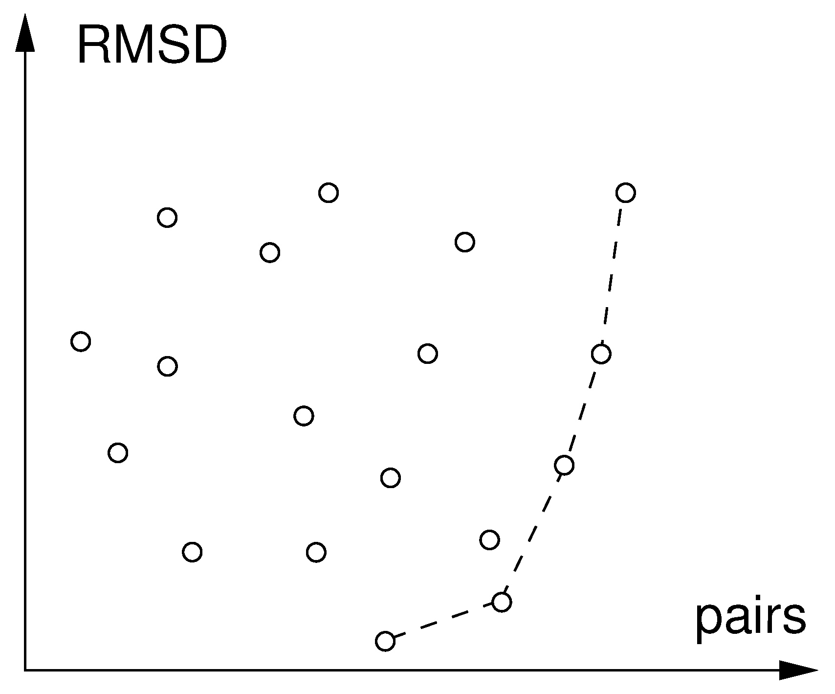
Steps 1 to 4 are carried out for all pairings of query epitope A with the 3D-structures $B_i$ in a database. Sizes of maximum common subgraphs (i.e. numbers of matched node pairs) and corresponding RMSD-values are collected for all these pairings. The set of matches that are not surpassed both in terms of low RMSD and high number of pairs constitute the set of Pareto-optimal matches or Pareto-front (Figure 4). Based on the structure of the Pareto-front, the user can then decide which matches are considered for further work. E.g. if there is a large gap in the Pareto-front between a low and a high RMSD-population but otherwise similar sizes of matched graphs, the user will prefer the matches with low RMSD. The plane shown in Figure 4 can be supplemented by accumulated P-scores from Step 3 as third dimension, resulting in a two-dimensional Pareto-front. In that case it is sensible to re-calibrate the P-scores with the maximum $S_{max}$ encountered in the database search.

Figure 4. Pareto-front of optimal matches found in database search. The circles connected by broken line are the set of Pareto-optimal matches. All other matches are (unconnected circles) are dominated by one of the members of the Pareto-optimal set as they have both lower RMSD and higher number of matched pairs.

Figure 4. Pareto-front of optimal matches found in database search. The circles connected by broken line are the set of Pareto-optimal matches. All other matches are (unconnected circles) are dominated by one of the members of the Pareto-optimal set as they have both lower RMSD and higher number of matched pairs.

2.3. Applications

In the following three subsections we demonstrate that EpitopeMatch can be successfully applied to different classes of problems. Protein structures used are taken from the Protein Data Bank (PDB) [1]. These tests have been carried out on a Intel Core 2 Duo processor running at 2.4 GHz with 4 GB RAM. For a benchmark with Assam see Section 2.4.

Matching two protein structures

The matching of two complete large molecular structures is a worst case scenario for EpitopeMatch since then Step 1, which dominates time complexity, becomes very large. Here we try to match the α-chain (141 amino-acids) and β-chains (146 amino-acids) of human hemoglobin, available as chains A and B under PDB-code 2DN2.

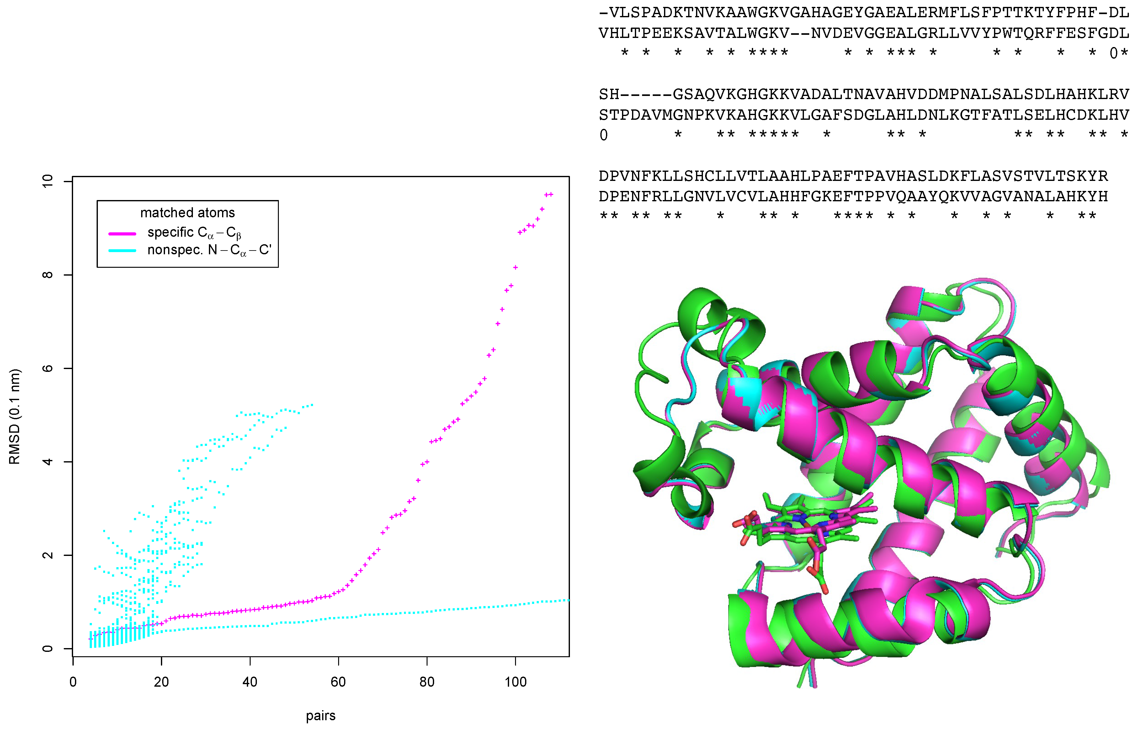
We have tested two different modes of matching. In the first (“unspecific”) we have matched protein backbone atoms N, $C_{\alpha }$, $C^{\prime }$ of all amino-acids irrespective of the type of amino-acids. In the second (“specific”) we have tried to match $C_{\alpha }$- and $C_{\beta }$-atoms with amino-acid types as attributes (for Gly $C_{\beta }$ is not considered). The plot in the left part of Figure 5 shows the unspecific and specific results as points colored in cyan and magenta, respectively. The plot does not only show RMSD and number of matched pairs of amino-acids for the largest common subgraph, but also for graphs that are obtained if node by node is removed from the largest common down to graphs of $\nu =4$ nodes, with each removed node having the lowest P-score in the respective graph. Thus the envelopes of the points in the plot towards low RMSD and high number of matches pairs also mark a kind of Pareto-front with a trade-off between low RMSD and low number of matched pairs up to high RMSD and high number of matched pairs.

In the unspecific mode, a maximum of 138 amino-acid pairs could be matched with a RMSD of 1.41 Å after a run of 173 s. Apart from matches of the full polypeptide chain, EpitopeMatch finds also matches of helices at different positions in the protein fold. These partial matches with low number of matched pairs and higher RMSD are displayed in the left part of Figure 5 as cloud of magenta points above the almost straight line of low-RMSD matches of the global fold.

Figure 5. Matching α- and β-chains of human hemoglobin. Left: matched pairs of amino-acids vs. RMSD after optimal superposition for two matching modes. Right bottom: optimal superposition of the match of β-chain (green) with α-chain matched using the amino-acid specific mode (magenta), and the unspecific mode (cyan). Right top: sequence alignment (α-chain in top row, β-chain in bottom row) derived from the structural alignment. Matching pairs of amino-acids are marked with asterisks.

Figure 5. Matching α- and β-chains of human hemoglobin. Left: matched pairs of amino-acids vs. RMSD after optimal superposition for two matching modes. Right bottom: optimal superposition of the match of β-chain (green) with α-chain matched using the amino-acid specific mode (magenta), and the unspecific mode (cyan). Right top: sequence alignment (α-chain in top row, β-chain in bottom row) derived from the structural alignment. Matching pairs of amino-acids are marked with asterisks.

The run in the specific mode took 52.46 s. Remarkably, the plot shows a kink at 61 matched pairs of amino-acids. At this point the RMSD is 1.26 Å. Below 61, the matched pairs are true positive matches in the helices of the two proteins. Above 61, the algorithm starts to match parts of the structurally and sequentially more divergent loop regions, including also false positives, i.e. amino-acids that of are of corresponding types but non-equivalent positions in the fold. We have from the matches up to the 61th pair derived a sequence alignment (top right of Figure 5). This alignment is almost identical to a pure sequence alignment with the Needleman-Wunsch algorithm with the Gonnet scoring matrix as implemented in ClustalW [13]. ClustalW finds as identities the 61 pairs found by EpitopeMatch,and additionally the two pairs marked with “0”.

The superimposed structures of both runs are shown in the lower right part of Figure 5. The the two chains are matched well in both modes.

Recognition of a binding site in a homolog

This example is a typical small scale application of EpitopeMatch. The protein Hst2 from yeast (PDB-code 1Q1A) and the human Sir2 protein (PDB-code 1MA3) are homologous and their 3D-structures have been determined experimentally. Both proteins bind the co-substrate ADP ribose and transfer an acetyl-group from a peptide-substrate to an ADP ribose to form 2’-O-acetyl-ADP-ribose (OAR). The structure of the complex of Hst2 with OAR is known, whereas the structure of the OAR complex with Sir2 is not known. Here we try to locate the OAR-binding pocket on Sir2 in the following way: We first define the OAR-binding epitope as the 20 amino-acid residues identified by Zhao et al. [14] in the structure of Hst2. Then, by using this epitope as query, we search for a match on the structure of Sir2.

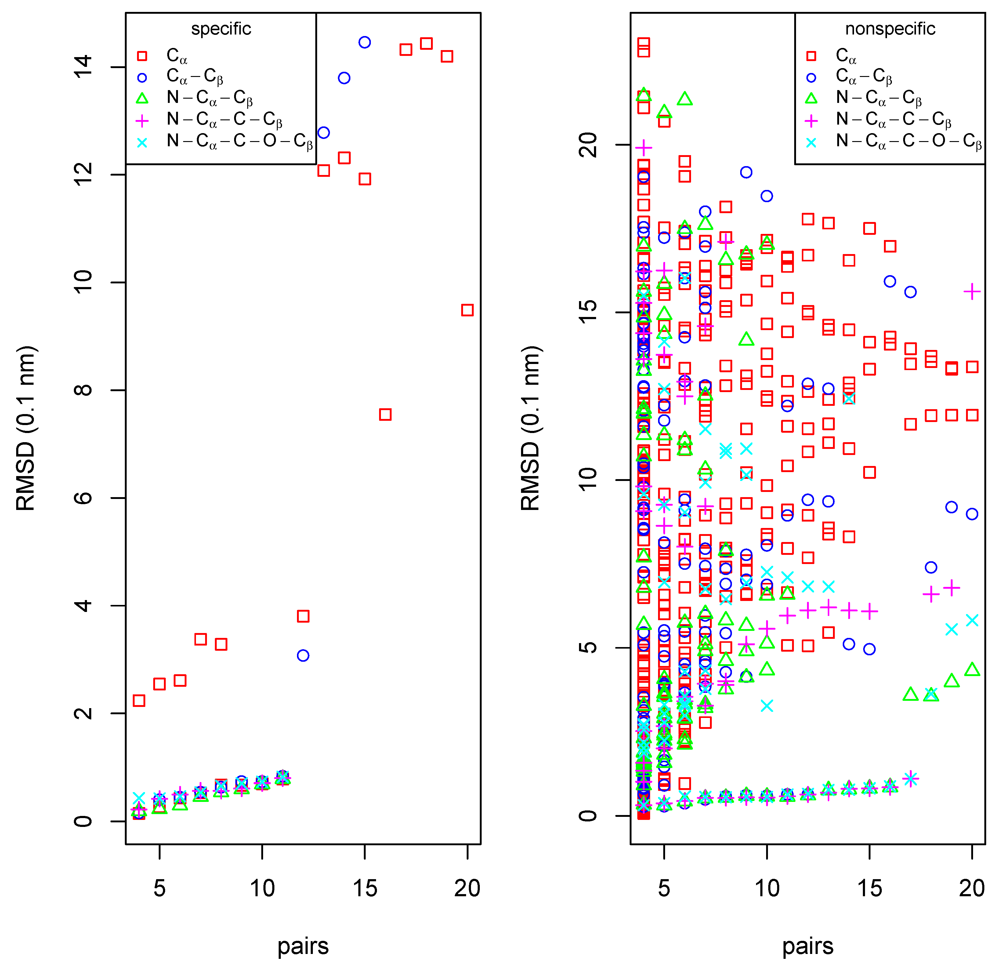
In this application we test the effectivity of a number of specific and unspecific search modes, each with five different sets of atoms per amino-acid. The results are shown in Figure 6). Run times per search were in the range of 2.3 min to 5.2 min, memory usage between 8 MB and 50 MB.

Figure 6. Results of amino-acid specific (left) and unspecific (right) searches for a match of the OAR binding epitope of yeast Hst2 on human Sir2 with various sets of atoms per residue.

Figure 6. Results of amino-acid specific (left) and unspecific (right) searches for a match of the OAR binding epitope of yeast Hst2 on human Sir2 with various sets of atoms per residue.

The amino-acid specific search identifies 11 of the 20 residues of the Hst2-epitope also in Sir2 if $C_{\beta }$-atoms are included (left part of Figure 6) at a RMSD of 1 Å. The unspecific search finds at an RMSD of less than 2 Å even 17 residue matches (right part of Figure 6). The 6 residues not found in the specific search are replaced in Sir2 by residues that are not too different (T37(Hst2) → A28(Sir2), F67→A51, T224→S192, L249→A218, Y269→K234, S270→A235). Both search modes show a distinct gap at 11 and 17 matched residues, respectively, giving a natural cutoff for the number of true matches. The non-specific search finds a noise of many false positive matches, while the true positive matches are separated from this noise by distinctly lower RMSD values.

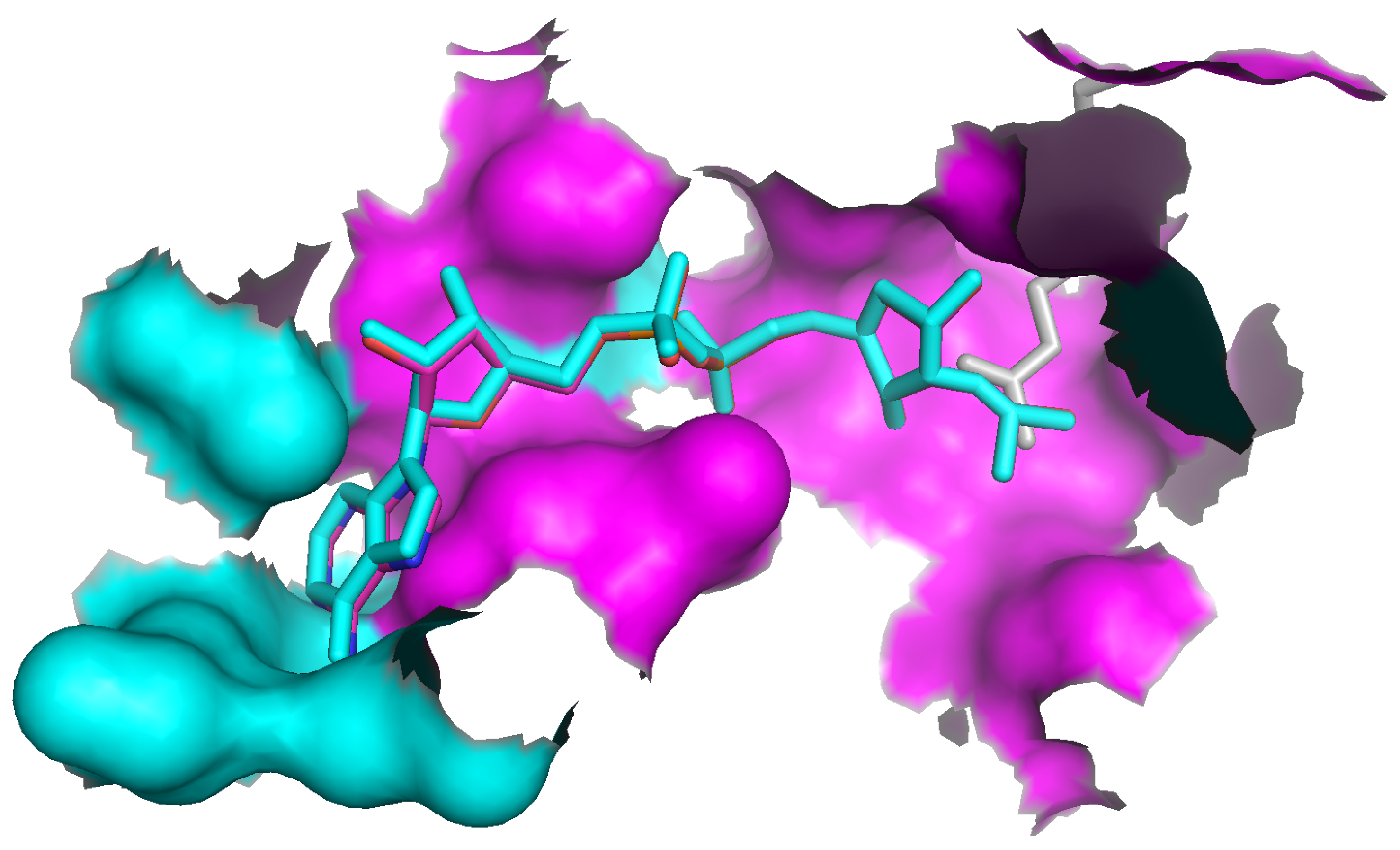
Figure 7 shows the parts of Sir2 that have been matched with the OAR binding epitope of Hst2. The residues matched in the unspecific mode (cyan and magenta) delineate the whole binding pocket of OAR, whereas the residues matched in the amino-acid specific mode (magenta) concentrate around the actual enzymatic site where the acetyl-group is transferred from a peptide to the OAR precursor. If the transformation that optimally superimposes the Hst2 epitope with the putative epitope in Sir2 (Step 4 of algorithm) is also applied to the OAR of Hst2, the transformed OAR fits well into the putative epitope pocket of Sir2. It is particularly remarkable that the position of the acetyl-group of OAR is very close to the position of an acetylated Lys residue of a substrate-peptide complexed with Sir2, supporting the correctness of the match.

Figure 7. The part of the human Sir2 protein structure (PDB-code 1MA3) matched with the OAR binding pocket of yeast Hst2. All 17 residues shown as molecular surface have been found as “unspecific” match. A subset of these (magenta) has been matched with the amino-acid specific mode. The molecule in sticks-representation in the center is OAR transformed into the empty binding pocket of Sir2 from the structure of the original complex with Hst2 using the co-ordinate transformation derived from the match (there are two very close OAR positions, derived from the specific and unspecific match, respectively). The grey sticks in the right half are an acetylated Lys residue of a substrate-peptide complexed with Sir2.

Figure 7. The part of the human Sir2 protein structure (PDB-code 1MA3) matched with the OAR binding pocket of yeast Hst2. All 17 residues shown as molecular surface have been found as “unspecific” match. A subset of these (magenta) has been matched with the amino-acid specific mode. The molecule in sticks-representation in the center is OAR transformed into the empty binding pocket of Sir2 from the structure of the original complex with Hst2 using the co-ordinate transformation derived from the match (there are two very close OAR positions, derived from the specific and unspecific match, respectively). The grey sticks in the right half are an acetylated Lys residue of a substrate-peptide complexed with Sir2.

Identification of a ligand binding site in a database

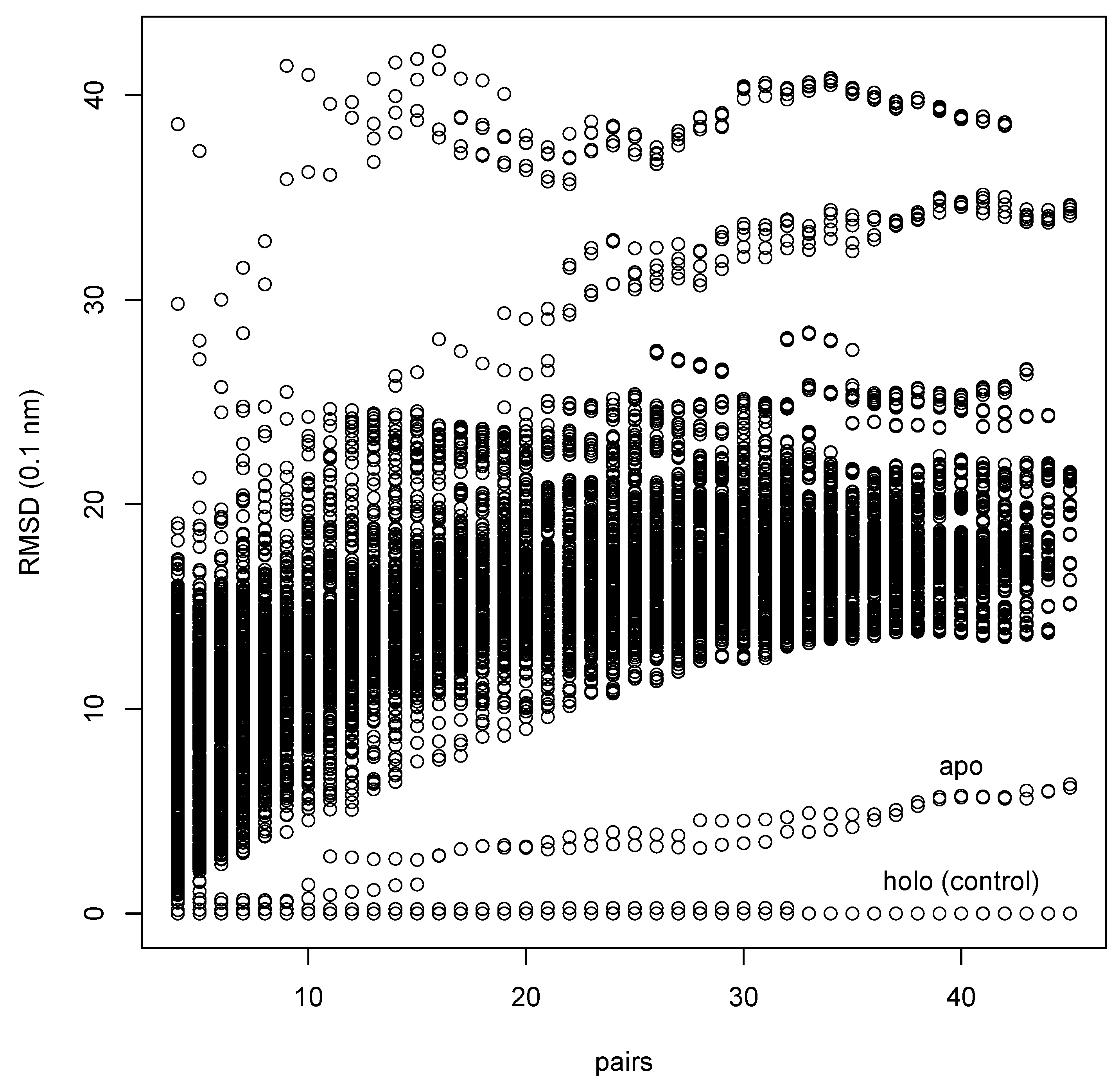
This is an example of a typical medium-to-large scale application of EpitopeMatch. We have taken a set of structures of pairs of apo-enzymes and the corresponding holo-enzymes compiled by Gunasekaran & Nussinov [16], excluding structures of more than 1000 amino-acids for reasons of memory restriction (see section 2.5.). The resulting set contains 86 pairs of proteins. The pair of holo- (PDB-code 1AKE) and apo-adenylate-kinase (PDB-code 4AKE) of E. Coli is part of the set. The protein is a dimer with two similar binding sites that experience a large induced fit on formation of a complex with inhibitor AP5.

Using the holo-structure, we define the query epitope by all 45 amino-acids with a distance of up to 5 Å to any atom of the inhibitor molecule. We are trying to find matches with this epitope in all 86 apo-proteins, including the holo-structure 1AKE as positive control. For the search we are using all N-,$C_{\alpha }$-,$C^{\prime }$-, and $C_{\beta }$-atoms and attribute them with the amino-acid types (“specific” search).

Figure 8 shows the accumulated results of the search in the same way as in Figure 5. The run needed a total of 49 min of CPU time, of which the investigation of 4AKE alone took 23 s (and 20 MB RAM). As expected, we find the two chains of the holo-structure 1AKE (“holo (control)”) as matches with vanishing RMSD for all graph sizes. The two chains of the correct apo-structure 4AKE (“apo” in figure) are found as by far the best matches in the set of 86 different apo-enzyme structures with a large gap in RMSD to the next best matches. It is notable that there is a clear match although the induced fit leads to a RMSD between the epitopes in 1AKE and 4AKE of more than 6 Å.

Figure 8. Search for an epitope in a database [16]. 86 structures of different apo-enzymes are searched for a match with a ligand binding pocket of 45 amino-acids. The source of the query epitope (1AKE) is included as control. The method identifies amongst the structures the one correct apo-structure (4AKE) as match with lowest RMSD (“apo”).

Figure 8. Search for an epitope in a database [16]. 86 structures of different apo-enzymes are searched for a match with a ligand binding pocket of 45 amino-acids. The source of the query epitope (1AKE) is included as control. The method identifies amongst the structures the one correct apo-structure (4AKE) as match with lowest RMSD (“apo”).

2.4. Comparative test

In terms of input and nature of results, the closest available relative of EpitopeMatch that we could find is Assam, though there are also clear differences, as e.g. Assam uses preprocessed data, whereas our code generates matches on the fly, which makes comparison of run-times misleading. Moreover, Assam uses the subgraph-isomorphism algorithm of Ullmann [15] whereas EpitopeMatch uses a heuristic that iteratively builds up larger and larger matches. Nevertheless, both methods promise to identify discontinuous epitopes similar to a given query epitope in a database of structures. Hence, we have tested the performance of both algorithms by means of the same benchmark application.

The test case is the search for epitopes that are similar to the maltose binding motif of the structure with PDB code 1ANF in all structures of the PDB (55534 molecular structures as of February 3, 2009). We assume that Assam did operate on essentially the same version of the database, which is plausible given many matches found by both methods (see Supplementary Material). In the PDB there are several other maltose binding proteins with similar binding pockets that should be found by the queries. The search pattern was formulated as set of $C_{\alpha }$ atoms and one atom representing each amino-acid side-chain (except for Glycine) of residues in the 5 Å-neighborhood of the maltose ligand in 1ANF. The full epitope comprised 17 atoms.

We have submitted the epitope of 1ANF to Assam via its web-service at http://grafss.imfr.net/assam/ (the program used was actually called Aspreg as of February 2, 2009, 18:17), and to EpitopeMatch. The latter was run on 16 cores of a Linux cluster (AMD Opteron 2218 2,6 GHz CPUs, each core with 4 GB RAM). Although the run times cannot be compared we give them here for completeness: Assam results were returned after 44h14m (for output see Supplementary Material), EpitopeMatch after 16h43m; because of the parallelization the total runtime of EpitopeMatch amounted to 267h20m.

All 55534 PDB entries were screened for the epitope by EpitopeMatch for matches of 7 to 17 atoms with the query epitope and a maximum RMSD of 3 Å. These conditions for minimum size of matches and maximum RMSD were in agreement with those reported by Assam. EpitopeMatch aborted in six cases of very large structures (2CSE, 1XI5, 1XI4, 1HTQ, 1N03, 1MFR) because of too large memory requirements. In 47658 PDB entries subgraph matches were located, in 7870 entries no subgraph matches could be found by EpitopeMatch. Of all subgraphs the above conditions were fulfilled for a small subset: 119 such epitopes were identified by EpitopeMatch in 89 PDB structures, 60 epitopes were identified by Assam in 26 PDB structures (Figure 9; see also Supplementary Material). The set of Assam matches was a subset of those found by EpitopeMatch.

Figure 9. Comparison of EpitopeMatch (black crosses) with Assam [9] (red crosses), with a PDB-wide search for epitopes similar to the maltose binding pocket in 1ANF formed by 17 atoms. Along the horizontal axis the names of the PDB structures in which MCS have been identified are given. The vertical axis gives above the zero line the number of matched atoms, below zero the corresponding RMSD.

Figure 9. Comparison of EpitopeMatch (black crosses) with Assam [9] (red crosses), with a PDB-wide search for epitopes similar to the maltose binding pocket in 1ANF formed by 17 atoms. Along the horizontal axis the names of the PDB structures in which MCS have been identified are given. The vertical axis gives above the zero line the number of matched atoms, below zero the corresponding RMSD.

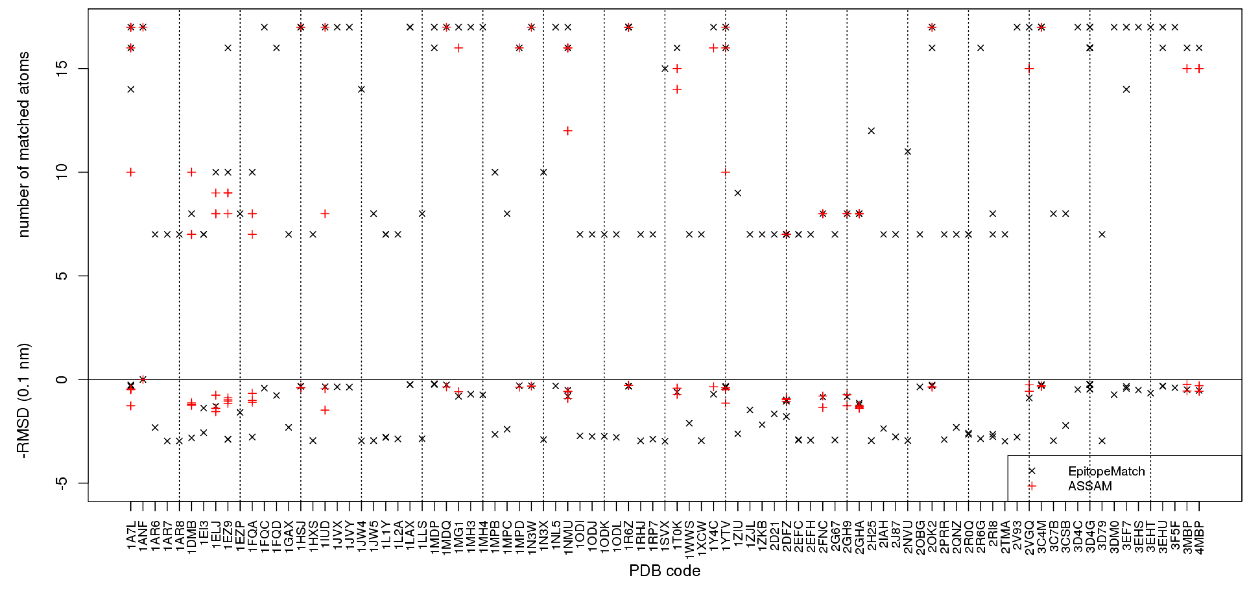
Figure 9 reveals several remarkable differences between the results of the two methods. The set of full matches of 17 atoms identified by Assam is a subset of those found by EpitopeMatch, more precisely, EpitopeMatch finds full matches in three times as many proteins as Assam. The set of full or almost full matches includes rather clear cases as the maltose binding proteins 1EZ9, 1LAX, or 1MDP. 1EZ9 is an interesting case since Assam finds matches of 8 and 9 atoms overlapping with the full binding motif, whereas EpitopeMatch finds a match of 10 atoms and a near-complete match of 16 atoms. This exemplifies a general tendency of EpitopeMatch that can be seen from Figure 9, namely that the size of graphs matched by EpitopeMatch is usually greater or equal to those found by Assam, the only exception being 1DMB. For most PDB structures where both methods identify matches, there is no clear winner in terms of RMSD values amongst the two methods.

Another notable difference is the occurrence of many smaller matches of 7 or 8 atoms with higher RMSD values of between 2 and 3 Å in the output of EpitopeMatch (Figure 9) whereas Assam identifies nothing in these PDB structures, although at least some of these are validated sugar binding proteins, such as 1JW4, 1JW5, or 2H25. 2V93 is a special case in which the two algorithms behave differently for trivial reasons: Assam ignores files without side-chain atoms; EpitopeMatch matches what can be matched even if atoms are missing.

We can conclude that due to the operation of Assam on preprocessed data, Assam probably beats EpitopeMatch in terms of CPU time for the actual search, whereas EpitopeMatch returns more and larger matches.

2.5. Discussion of practical performance

EpitopeMatch has been implemented in Java 1.6. Java is certainly not the preferred language for large scale computing tasks. Nevertheless, the performance in terms of computing time is satisfactory in all considered cases. As shown in the benchmark application, the algorithm can be easily parallelized with practically linear scaling at various levels. EpitopeMatch can be outperformed by specialized codes such as Daliif explicit use of higher level organization is made, such as secondary structure. On the other hand, such specialized codes typically cannot identify discontinuous epitopes, which is more the application intended for EpitopeMatch.

EpitopeMatchhas still many options for improvements towards more efficient use of time and memory. E.g. we have observed that relatively bad matches in the first iterations of the algorithm usually do not lead to good matches in later iterations. Therefore, in database searches, the efficiency can be increased further by the introduction of an early break of iterations if no cliques are found at low distance tolerances. In the current implementation of EpitopeMatchmemory usage is critical for searches of large epitopes in large proteins of several thousand amino-acids, and we have experienced in such cases occasional memory overflows on machines with 4 GB RAM.

In terms of effectivity, the algorithm performs well, identifying good matches in different application scenarios from whole molecule matching to the matching of epitopes with a considerable flexibility, e.g. due to induced fit. Effectivity can be influenced strongly by considering more than one center per residue. Our implementation allows this, as demonstrated in Figure 5 and Figure 6. All these atoms are matched in parallel, and the CPU-time increases roughly linear with number of atoms per residue taken into account.

We have already introduced some of the optimization measures to further increase effectivity and time efficiency, so that the code currently available from the authors does not only identify more matches but also is about three times faster than that used in the above benchmark.

3. Supplementary material

Detailed outputs of Assam and EpitopeMatch in the benchmark application are provided as Supplementary Material. The compressed file contains a description (description.pdf) of the supplementary files, and output files of both programs. The full output of EpitopeMatch (several 100 MB) in the benchmark application and the EpitopeMatch code under the GNU General Public License are available from the authors.

References and Notes

- Berman, H.M.; Westbrook, J.; Feng, Z.; Gilliland, G.; Bhat, T.N.; Weissig, H.; Shindyalov, I.N.; Bourne, P.E. The Protein Data Bank. Nucleic Acids Res. 2000, 28, 235–242. [Google Scholar] [CrossRef] [PubMed]
- Gronwald, W.; Hohm, T.; Hoffmann, D. Evolutionary Pareto-optimization of stably folding peptides. BMC Bioinformatics 2008, 9. [Google Scholar] [CrossRef] [PubMed]
- Lemmen, C.; Lengauer, T. Computational Methods for the Structural Alignment of Molecules. J. Comput. Aided. Mol. Des. 2000, 14, 215–232. [Google Scholar] [CrossRef] [PubMed]
- Halperin, I.; Ma, B.; Wolfson, H.; Nussinov, R. Principles of Docking: An Overview of Search Algorithms and a Guide to Scoring Functions. Proteins 2002, 47, 409–443. [Google Scholar] [CrossRef] [PubMed]
- Holm, L.; Sander, C. Protein Structure Comparison by Alignment of Distance Matrices. J. Mol. Biol. 1993, 233, 123–138. [Google Scholar] [CrossRef] [PubMed]
- Taylor, W.R.; Orengo, C.R. Protein Structure Alignment. J. Mol. Biol. 1989, 208, 1–22. [Google Scholar] [CrossRef]
- Norel, R.; Fischer, D.; Wolfson, H.J.; Nussinov, R. Molecular Surface Recognition by a Computer vision-based Technique. Protein Eng. 1994, 7, 39–46. [Google Scholar] [CrossRef] [PubMed]
- Raymond, J.W.; Willett, P. Maximum Common Subgraph Isomorphism Algorithms for the Matching of Chemical Structures. J. Comput.-Aided Mol. Des. 2002, 16, 521–533. [Google Scholar] [CrossRef] [PubMed]
- Artymiuk, P.J.; Poirrette, A.R.; Grindley, H.M.; Rice, D.W.; Willett, P. A Graph-theoretic Approach to the Identification of Three-dimensional Patterns of Amino Acid Side-chains in Protein Structures. J. Mol. Biol. 1994, 243, 327–344. [Google Scholar] [CrossRef] [PubMed]
- Varkony, T.; Shiloach, Y.; Smith, D. Computer-Assisted Examination of Chemical Compounds for Structural Similarities. J. Chem. Inf. Comput. Sci. 1979, 19, 104–111. [Google Scholar] [CrossRef]
- Bron, C.; Kerbosch, J. Algorithm 457: Finding All Cliques of an Undirected Graph. Comm. of the ACM 1973, 16, 575–577. [Google Scholar] [CrossRef]
- Kabsch, W. A Solution for the Best Rotation to Relate Two Sets of Vectors. Acta Cryst. 1976, 922, 922–923. [Google Scholar] [CrossRef]
- Thompson, J.D.; Higgins, D.G.; Gibson, T.J. CLUSTAL W: Improving the Sensitivity of Progressive Multiple Sequence Alignment through Sequence Weighting, Positions-Specific Gap Penalties and Weight Matrix Choice. Nucl. Acids Res. 1994, 22, 4673–4680. [Google Scholar] [CrossRef] [PubMed]
- Zhao, K.; Chai, X.; Marmorstein, R. Structure of the Yeast Hst2 Protein Deacetylase in Ternary Complex with 2’-O-Acetyl ADP Ribose and Histone Peptide. Structure 2003, 11, 1403–1411. [Google Scholar] [CrossRef] [PubMed]
- Ullmann, J.R. An Algorithm for Subgraph Isomorphism. J. Assoc. Comput. Machinery 1976, 16, 31–42. [Google Scholar] [CrossRef]
- Gunasekaran, K.; Nussinov, R. How Different are Structurally Flexible and Rigid Binding Sites? Sequence and Structural Features Discriminating Proteins that Do and Do not Undergo Conformational Change upon Ligand Binding. J. Mol. Biol. 2007, 365, 257–273. [Google Scholar] [CrossRef] [PubMed]