Coarsely Quantized Decoding and Construction of Polar Codes Using the Information Bottleneck Method

Abstract

The information bottleneck method is a generic clustering framework from the field of machine learning which allows compressing an observed quantity while retaining as much of the mutual information it shares with the quantity of primary relevance as possible. The framework was recently used to design message-passing decoders for low-density parity-check codes in which all the arithmetic operations on log-likelihood ratios are replaced by table lookups of unsigned integers. This paper presents, in detail, the application of the information bottleneck method to polar codes, where the framework is used to compress the virtual bit channels defined in the code structure and show that the benefits are twofold. On the one hand, the compression restricts the output alphabet of the bit channels to a manageable size. This facilitates computing the capacities of the bit channels in order to identify the ones with larger capacities. On the other hand, the intermediate steps of the compression process can be used to replace the log-likelihood ratio computations in the decoder with table lookups of unsigned integers. Hence, a single procedure produces a polar encoder as well as its tailored, quantized decoder. Moreover, we also use a technique called message alignment to reduce the space complexity of the quantized decoder obtained using the information bottleneck framework.

1. Introduction

In a typical transmission chain, forward error correction is a resource-hungry and computationally complex component. Therefore, it is always desirable to reduce the decoder’s complexity. The commonly used soft decision decoders perform many intensive arithmetic operations on soft values, i.e., log-likelihood ratios (LLRs). In practice, the computational complexity of a decoder is reduced by replacing the intensive operations with simpler approximations. The space complexity of the decoder, i.e., the memory for storing the soft values and the number of wires for exchanging them between hardware components, depends on the representation of the soft values in the hardware. The space complexity of the decoder is reduced by coarsely quantizing the soft values where each soft value is represented using a small number of bits. These complexity reduction measures degrade the error-correcting performance of a decoder to some extent.

An interesting remedy for reducing the decoder complexity of low-density parity-check (LDPC) codes was presented in [1,2], where a quantized decoder for regular LDPC codes was developed using the information bottleneck method [3,4]. The design principle of such a quantized decoder combines the information bottleneck method with discrete density evolution [5]. Discrete density evolution is the quantized counterpart of density evolution [6], an analysis tool for LDPC codes. In the quantized decoder design of [1], referred to as the information bottleneck decoder here, the information bottleneck method is used to design mappings between the quantized input and output messages of each node in the Tanner graph of the code which maximize the mutual information between the outgoing messages and the bits they correspond to. Consequently, all the node operations in the information bottleneck decoder are deterministic mappings that can be realized as simple table lookups. Further, the decoder can be implemented using only unsigned integer arithmetic since all the quantized messages are unsigned integers. Moreover, no internal high resolution is needed for the node operations. Surprisingly, the computational simplicity of the information bottleneck decoders causes only a minute degradation in the error rate as compared to a double-precision floating-point sum-product decoder. It was reported that an information bottleneck decoder having a bitwidth as low as 4 bits performs very close to the belief propagation decoder [1]. The idea of information bottleneck decoders was extended to irregular LDPC codes in [7,8]. Design of quantized message passing decoders that utilize information preserving table lookup operations was also addressed in [9,10,11,12].

Results of [1,2,7,12] encourage to explore the application of the information bottleneck method in polar codes [13], an important class of channel codes that are seen as a breakthrough in the coding theory. They are the first linear block codes that can provably achieve the symmetric capacity of binary input memoryless channels. Despite being asymptotically good, the error correcting performance of polar codes at practical block lengths under successive cancellation (SC) [13] decoding is not impressive. This ordinary performance of polar codes was partly due to their weak Hamming distance properties [14,15] and partly due to the SC decoder being suboptimal [16]. To circumvent these issues, the authors in [16] proposed a serial concatenation of the polar code with an outer cyclic redundancy check (CRC) code and the use of the successive cancellation list (SCL) decoder. On the one hand, the SCL decoder is more powerful than the originally proposed SC decoder. On the other hand, the outer CRC code improves the distance properties of the polar code as observed in [17]. The resulting CRC-aid successive cancellation list decoding scheme can outperform state-of-the-art coding schemes. The outer CRC code can also be replaced with generalized parity check codes [18], resulting in parity check aided SCL decoding. Eventually, polar codes were included in the 5G standard for control channels in the eMBB scenario [19]. Although proposals for using other decoders, e.g., belief propagation for improving performance of polar codes appeared in the literature as early as [20], the CRC or parity check aided SCL decoder remains the practical decoding choice [21].

Polar codes exploit the channel polarization phenomenon where the effective channels, known as the bit channels, experienced by the bits at the input of the polar encoder exhibit polarized behavior: The bit channels tend to be either extremely reliable or completely unreliable. The code uses the reliable bit channels to carry information bits, whereas the input of the unreliable bit channels is fixed to predetermined values. Hence, the order of the bit channels with respect to their reliabilities is determined in order to identify the most reliable ones, a process commonly referred to as code construction. This order of the bit channels is not universal and depends on the underlying physical channel. For channel models of practical importance, e.g., AWGN channels, the output alphabet of the bit channels expands exponentially in the codeword length, making exact and efficient computation of the bit channel reliabilities challenging. Therefore, approximate construction methods are used for such channel models.

An important contribution regarding approximate construction methods was made in [22], where it was shown that the density evolution tool can also be used for the construction of polar codes. However, the precision requirements for an exact implementation of the method of [22] become impractical as the codeword length increases. The idea of [22] was extended by Tal and Vardy in [23], where they provided an efficient implementation of the quantized density evolution for polar code construction. In order to keep track of the inaccuracy introduced by the quantization, the method of [23] determines an upper and a lower bound on the probability of error of each bit channel. Performing the density evolution under a Gaussian approximation provides another notable construction method [24] that tracks the reliability of each bit channel using a single scalar quantity instead of its transition probabilities, hence considerably reducing the computation complexity of density evolution. For a binary input AWGN channel, the sets of reliable bit channels of polar codes constructed with the Gaussian approximation and the Tal and Vardy method differ only in few elements.

The idea of combining the information bottleneck method with density evolution [1] can also be utilized for polar code construction. However, unlike other construction methods, the benefits of this approach are twofold: Firstly, the discrete density evolution using the information bottleneck method compresses the output alphabet of the bit channels of a polar code to a small size, while minimizing the information loss due to the compression as much as possible. This compression facilitates computing the reliabilities of the bit channels in terms of their capacities, keeping track of the loss of the mutual information caused by the quantization [25]. Secondly, the intermediate steps of the discrete density evolution provide deterministic mappings between the quantized input and output messages for each node in the Tanner graph of the polar code. These deterministic mappings can replace the LLR computations of a conventional decoder, constituting an information bottleneck SC or SCL decoder [26]. Hence, a polar code and its tailored quantized decoder are obtained from the same process. Similar to the information bottleneck LDPC decoders [1,7], all the operations in the information bottleneck SC decoder are table lookups of unsigned integers. However, the path metric computation in an information bottleneck SCL decoder is done similar to that in a conventional decoder as in [27]. The error rate of a 4-bit information bottleneck SCL decoder is only slightly worse than that of a double-precision floating-point SCL decoder. The lookup tables used in the information bottleneck SCL decoders are categorized into decoding and translation tables. The decoding tables are used for the successive cancellation part of the decoder, while the translation tables are used to translate the integer valued messages into LLRs for path metric updates. For a codeword length N, $2N-2$ distinct decoding tables and N distinct translation tables are used [26]. Thus, the space complexity of an information bottleneck SCL decoder increases with the codeword length N.

Quantized SC and SCL decoders have been studied in, e.g., [27,28,29,30,31]. There are two major differences between these quantization approaches from the literature and the one proposed in this paper. Firstly, unlike the aforementioned quantization approaches, the quantization performed using the information bottleneck method is nonuniform in nature. Secondly, the quantization in [27,28,29,30,31] assigns a numerical value, e.g., reconstructed from the quantization labels, to each quantized LLR, which is then used in the relevant arithmetic operation. By contrast, the information bottleneck SCL decoder works entirely with the integer valued quantization labels and translates them into LLRs only when required, i.e., for path metric update. In addition to addressing the trade-off between quantization bitwidth and rate loss of an SC decoder, the authors in [28] proposed a very coarse 3-level, i.e., 2-bit, quantization scheme. Moreover, it was shown that the performance loss caused by the quantization is more pronounced for low code rates. The 3-level quantization scheme of [28] was deployed in short block length polar codes in [31], where it leads to significant degradation in the error rate. However, the author proposed improvements to the SCL decoder which drastically reduce this degradation.

In this paper, we present the polar code construction using the information bottleneck method [25] in detail, along with its comparison to the closely related construction method of Tal and Vardy. Afterwards, the information bottleneck decoders of [26] are reviewed accompanied by detailed insights into their working. The huge number of lookup tables used in the information bottleneck decoders of [26] can be viewed as a space complexity cost for their computational simplicity. We demonstrate that using the message alignment technique of [7], the required number of tables and, hence, the space complexity of the information, bottleneck SCL decoders can be reduced.

The rest of the paper is structured as follows. After a brief recap of polar codes and the information bottleneck method in Section 2, polar code constructing using the information bottleneck method and Tal and Vardy’s method is discussed in Section 3. Section 4 shows how the results of Section 3 are used for decoding. Section 5 presents our latest work on the subject: space complexity reduction of the information bottleneck SCL decoder. Section 6 presents simulation results before concluding the paper in Section 7.

Notations

Random variables are denoted by capital italic font, e.g., X with realizations $x\in \mathcal{X}$. $I(X;Y)$, $p\left(y\right|x)$ and $p(x,y)$ represent the mutual information, conditional probability, and joint probability distribution of the two random variables X and Y. Multivariate random variables are represented with capital bold italic font, e.g., $\mathit{Y}={[Y_0,Y_1]}^T$. Matrices are represented with capital bold font, e.g., $\mathbf{Y}$, and vectors are represented using a lower case bold font, e.g., $\mathbf{y}$. All vectors are column vectors.

2. Prerequisites

This section presents a brief recap of the relevant aspects of polar codes and introduces the information bottleneck framework.

2.1. Polar Codes

A polar code with length $N=2^n$, where $n=1,2\dots$, is described by its $N\times N$ generator matrix

$$\begin{array}{c}\hfill {\mathbf{G}}_N={\mathbf{F}}^{\otimes n}\mathbf{B},\end{array}$$

(1)

where matrix $\mathbf{F}=\left[\begin{array}{cc}1& 1\\ 0& 1\end{array}\right]$ and $\mathbf{B}$ is the bit reversal permutation matrix [13]. While the encoding follows $\mathbf{x}={\mathbf{G}}_N\mathbf{u}$, the FFT-like structure of ${\mathbf{F}}^{\otimes n}$ allows efficient encoding with a complexity of $O\left(N{log}_{2}N\right)$. For a code rate of $K/N$, $(N-K)$ bits in the encoder input $\mathbf{u}={[u_0,\dots ,u_{N-1}]}^T$ are set to fixed values, e.g., 0’s, and referred to as frozen bits. The values and location of the frozen bits are known to the decoder. The remaining K positions in u, specified in the information set, $\mathcal{A}$, carry the information bits.

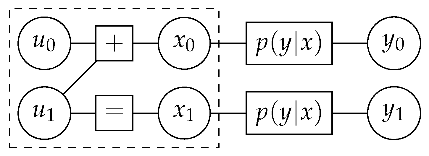
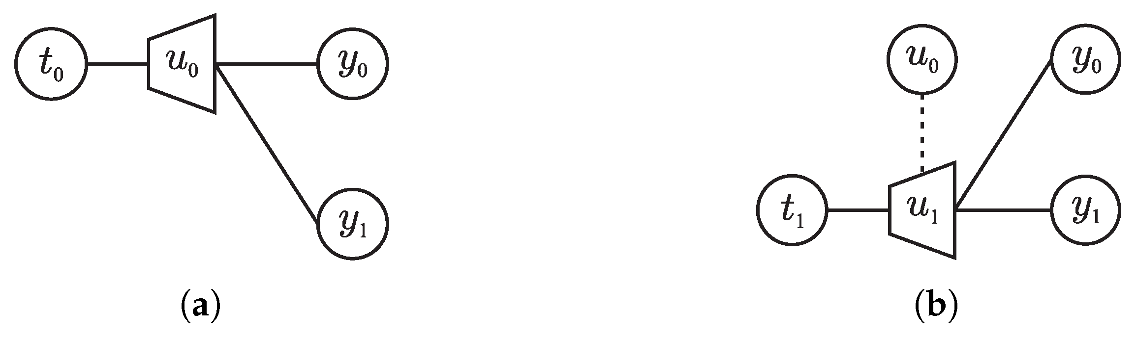
The matrix $\mathbf{F}$ serves as the building block of polar codes in the sense that all the processing steps required for encoding, code construction, and decoding are defined over it. From an encoding perspective, $\mathbf{F}$ encodes the bits in $\mathbf{u}={[u_0,u_1]}^T$ into codeword $\mathbf{x}={[x_0,x_1]}^T$, which is received as $\mathbf{y}={[y_0,y_1]}^T$ after transmission through a symmetric discrete memoryless channel described by transition probabilities $p\left(y\right|x)$. Figure 1 depicts the factor graph of this elementary setup of polar codes. The key concept of polar codes lies in the definition of virtual bit channels between each element in $\mathbf{u}$ and the channel output, $\mathbf{y}$. Two bit channels are defined over the building block. The first bit channel, described by transition probabilities $p(y_0,y_1|u_0)$, is established between ${\mathbf{y}}_0={[y_0,y_1]}^T$ and $u_0$ and ignores $u_1$:

$$p\left({\mathbf{y}}_0\right|u_0)=\frac{1}{2}\sum _{u_1\in \left\{0,1\right\}}p\left(y_0\right|u_0\oplus u_1)p\left(y_1\right|u_1).$$

(2)

The second virtual channel, described by transition probabilities $p(y_0,y_1,u_0|u_1)$, treats $u_1$ as input and ${\mathbf{y}}_1={[y_0,y_1,u_0]}^T$ as output, assuming the true knowledge of $u_0$:

$$p\left({\mathbf{y}}_1\right|u_1)=\frac{1}{2}p\left(y_0\right|u_0\oplus u_1)p\left(y_1\right|u_1).$$

(3)

If $P_e,P_e^0$, and $P_e^1$ are the probabilities of error of the physical channel, the bit channel of $u_0$ and the bit channel of $u_1$, respectively, then $P_e^0\ge P_e\ge P_e^1$ [13]. Hence, the setup of Figure 1 transforms two instances of the physical channel into qualitatively different synthetic channels.

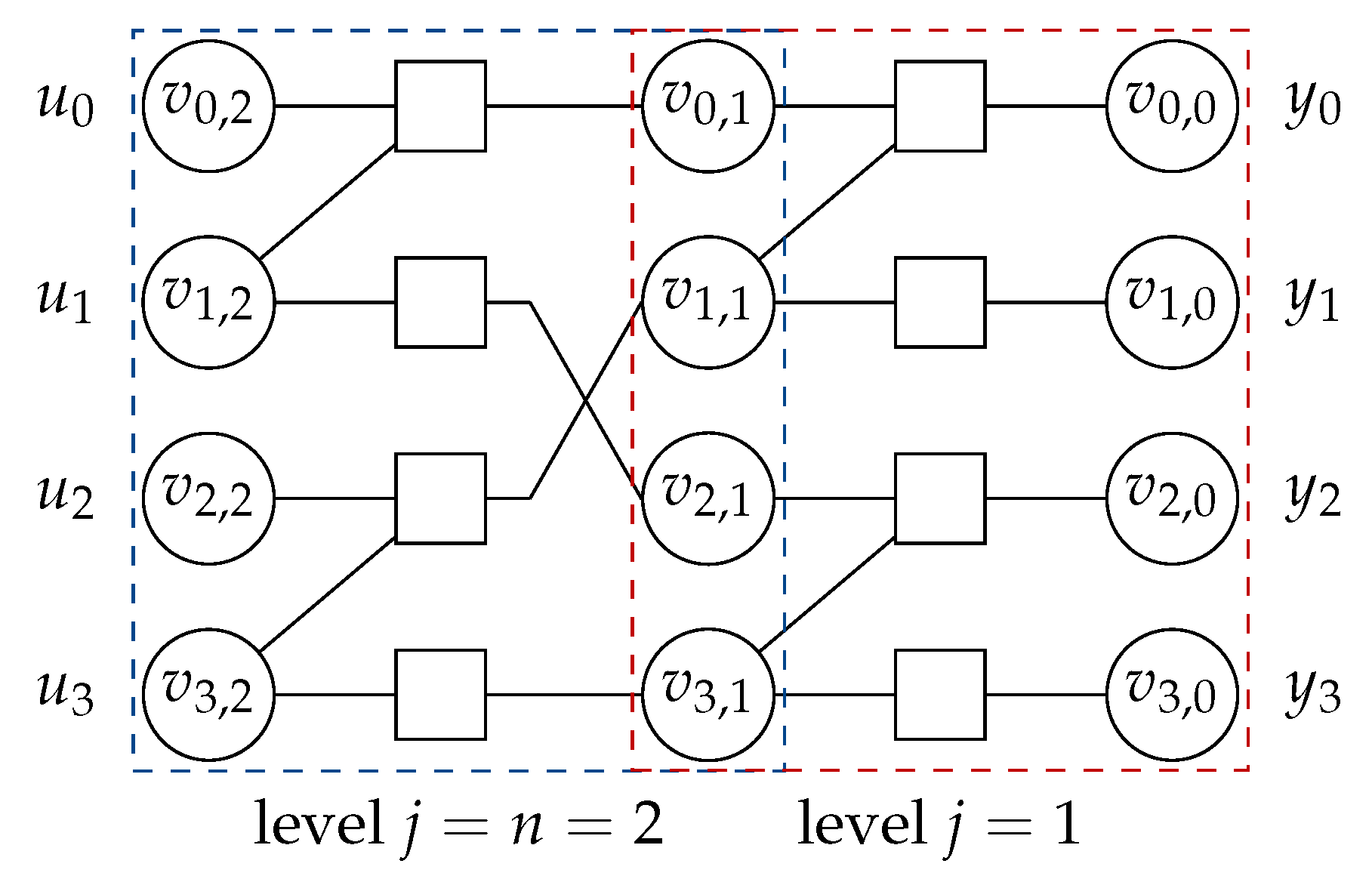
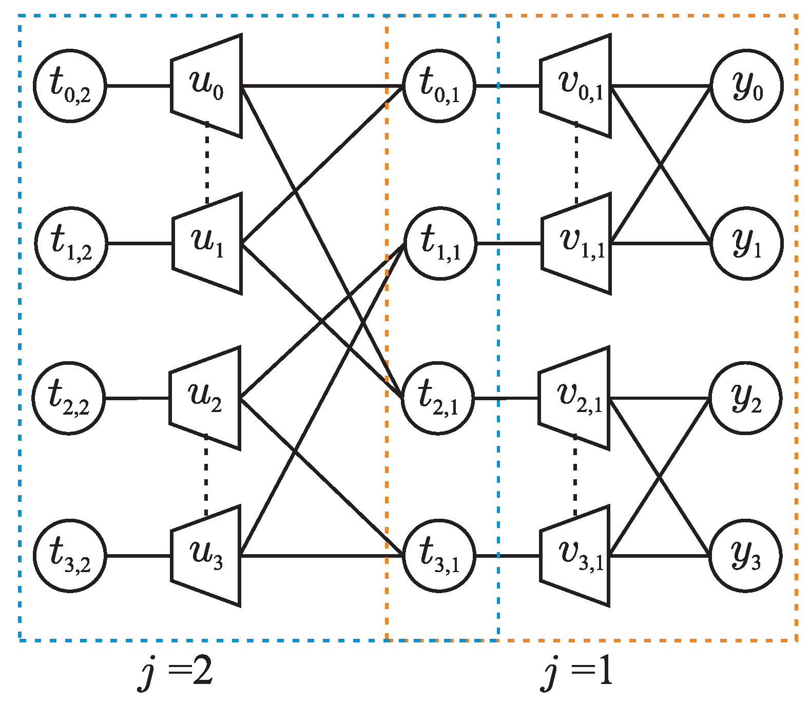
Figure 2 shows the factor graph of a polar code for $N=4$, where the transmission channel is implicitly included, i.e., the right-most variable nodes correspond to received coded bits. The code structure is composed of the building blocks arranged in vertical columns, referred to as levels, j, with right-most being $j=1$ and left-most being $j=n$. Within a level j, variable nodes to the left of the check nodes are labeled with j, while those on the right of the check nodes are labeled with the level $j-1$. Thus, every variable node has a label $v_{i,j}$ with $i=0,1,\dots ,N-1$ and $j=0,\dots ,n$. Then, $v_{i,n}$ are the encoder inputs $u_i$ and $v_{i,0}$ are the channel outputs $y_i$. It can be seen in Figure 2 that bit channels of a polar code are obtained after recursive application of the polarizing transform of Figure 1. Each application of the polarization transform at level j in the code structure manufactures a pair of bit channels from a pair of qualitatively similar (bit) channels from level $j-1$, similar to Equations (2) and (3), where the bit channel corresponding to the upper branch is worse, while the one corresponding to the lower branch is better.

The bit channels for a polar code with $N>2$ are the effective channels experienced by the individual bits $u_i$ under successive cancellation decoding where the true values of $u_0,\dots ,u_{i-1}$ are provided by a helpful genie regardless of any previous decoding error, and the bits $u_{i+1},\dots ,u_{N-1}$ are treated as unknowns. The transition probabilities of the bit channel of $u_i$ with equilikely inputs are given as:

$$p\left({\mathbf{y}}_i\right|u_i)=\sum _{u_{i+1},\dots ,u_{N-1}}\frac{1}{2^{N-1}}p\left(\mathbf{y}\right|\mathbf{x}),$$

(4)

where the concise notation ${\mathbf{y}}_i={\left[\mathbf{y},u_0,\dots ,u_{i-1}\right]}^T$ is used for the bit channel output, and $\mathbf{x}={\left[x_0,x_1,\dots ,x_{N-1}\right]}^T$ is the codeword.

2.2. Successive Cancellation List Decoder

The SC decoder works on the structure of Figure 2 and estimates the bit values $u_i$ in a sequential manner from $i=0$ to $N-1$. At each decoding stage i, ${\widehat{u}}_i$ is determined as:

$${\widehat{u}}_i=\left\{\begin{array}{cc}{u}_i\hfill & i\notin \mathcal{A}\hfill \\ 0\hfill & i\in \mathcal{A}\mathrm{and}{L}_{u_i}\left({\mathbf{y}}_i\right)\ge 0\hfill \\ 1\hfill & i\in \mathcal{A}\mathrm{and}{L}_{u_i}\left({\mathbf{y}}_i\right)<0,\hfill \end{array}\right.$$

(5)

where $L_{u_i}\left({\mathbf{y}}_i\right)=log\frac{p\left({\mathbf{y}}_i\right|u_i=0)}{p\left({\mathbf{y}}_i\right|u_i=1)}$ is the LLR of the bit $u_i$, and $\mathcal{A}$ denotes the information set. When ties in the case of $L_{u_i}\left({\mathbf{y}}_i\right)=0$ are broken randomly, Equation (5) is a maximum likelihood decoding of the ith bit channel. The LLR $L_{u_i}\left({\mathbf{y}}_i\right)$ is computed from subsequent levels in recursive steps as follows:

$$L_{v_{i,j}}\left({\mathbf{y}}_{i,j}\right)=\{\begin{array}{lll}{L}_{v_{i^{\prime },j-1}}\left({\mathbf{y}}_{i^{\prime },j-1}\right)⊞L_{v_{i^{″},j-1}}\left({\mathbf{y}}_{i^{″},j-1}\right)& i\mathrm{is}\mathrm{even}& \hspace{1em}\text{(6a)}\\ b_{i,j-1}{L}_{v_{i^{\prime },j-1}}({\mathbf{y}}_{i^{\prime },j-1}+L{v}_{i^{″},j-1}\left({\mathbf{y}}_{i^{″},j-1}\right)& i\mathrm{is}\mathrm{odd}& \hspace{1em}\text{(6b)}\end{array}$$

with $i^{\prime }=\lfloor \frac{i}{2}\rfloor +\lfloor \frac{i}{2^j}\rfloor 2^{j-1},i^{″}=i^{\prime }+2^{j-1}$ and $b_{i,j}={(-1)}^{{\widehat{v}}_{i-1,j}}$, where the bit value ${\widehat{v}}_{i-1}$ is available from the previous decoding stages. ${\mathbf{y}}_{i,j}$ represents output of the intermediate bit channel experienced by $v_{i,j}$. The ⊞ operator for two LLR values $L_1$ and $L_2$ is defined as [32]:

$$\begin{array}{c}\hfill L_1⊞L_2=log\frac{1+e^{L_1}{e}^{L_2}}{e^{L_1}+e^{L_2}}.\end{array}$$

(7)

The LLR values $L_{v_{i,0}}\left({\mathbf{y}}_{i,0}\right)$ in the recursion are given by the channel LLRs:

$$\begin{array}{c}\hfill L_{x_i}^{ch}\left(y_i\right)=log\frac{p\left(y_i\right|x_i=0)}{p\left(y_i\right|x_i=1)}.\end{array}$$

(8)

The successive cancellation list decoder can be viewed as $N_L$ successive cancellation decoders working in parallel. In SCL decoding, every time an estimate ${\widehat{u}}_i$ for $i\in \mathcal{A}$ has to be made, the decoder proceeds as an SC decoder for both possible decisions of ${\widehat{u}}_i$, instead of using Equation (5). The decoder maintains a list of possible decoding results where the number of decoding paths doubles after estimation of each information bit. If at any stage, the number of decoding paths in the list exceeds the maximum allowed list size, $N_L$, the decoder retains only the $N_L$ most likely decoding paths, dropping the rest. The likelihood of path $l\in \left\{0,1,\dots ,N_L-1\right\}$ in the list at stage i is captured by the path metric $M_{i,l}$ [27]:

$$M_{i,l}=M_{i-1,l}+ln(1+e^{-(1-2{\widehat{u}}_{i,l})L_{u_i}{\left({\mathbf{y}}_i\right)}_l}),$$

(9)

where $M_{i-1,l}$ is the metric of the lth path at decoding stage $i-1$, ${\widehat{u}}_{i,l}$ is the bit value with which the path is being extended, and $L_{u_i}{\left({\mathbf{y}}_i\right)}_l$ is the LLR value $L_{v_{i,j=n}}\left({\mathbf{y}}_{i,j=n}\right)$ for the lth path according to Equation (6). The path with the smallest metric is the most likely decoding path. The path increment $\Delta M_{i,l}=ln(1+e^{-(1-2{\widehat{u}}_{i,l})L_{u_i}\left({\mathbf{y}}_i\right)})$ is well-approximated as [27]:

$$\Delta M_{i,l}=\left\{\begin{array}{cc}0\hfill & \mathrm{if}{\widehat{u}}_{i,l}=\frac{1}{2}(1-\mathrm{sign}\left(L_{u_i}\left({\mathbf{y}}_i\right)\right)\hfill \\ |L_{u_i}\left({\mathbf{y}}_i\right)|\hfill & \mathrm{otherwise},\hfill \end{array}\right.$$

(10)

where sign $\left(L_{u_i}\left({\mathbf{y}}_i\right)\right)$ denotes the sign of the LLR value $L_{u_i}\left({\mathbf{y}}_i\right)$.

After the last decoding stage, i.e., $i=N-1$, the most likely decoding path from the list is selected as the decoder output. In the CRC-aided settings, a CRC checksum of $N_{crc}$ bits is appended after the K information bits, and the $K+N_{crc}$ bits are then polar encoded into an N bit codeword. The decoder output is then the most likely decoding path in the final list that passes the CRC check.

2.3. Polar Code Construction

The process of determining the position of information bits in $\mathbf{u}$ is known as code construction. Ideally, the K qualitatively best bit channels are included in the information set $\mathcal{A}$ during the code construction phase. The quality of the bit channels can be quantified in terms of their error probability or capacity, both of which can be computed from their transition probabilities. The probability of error, $P_e^i$, of the ith bit channel is computed as ([23], Equation (13)):

$$P_e^i=\frac{1}{2}\sum _{{\mathbf{y}}_i}min\left\{p\left({\mathbf{y}}_i\right|u_i=0),p\left({\mathbf{y}}_i\right|u_i=1)\right\},$$

(11)

while, its (symmetric) capacity is given by the mutual information $I(U_i;{\mathbf{Y}}_i)$:

$$I(U_i;{\mathbf{Y}}_i)=\frac{1}{2}\sum _{u_i}\sum _{{\mathbf{y}}_i}p\left({\mathbf{y}}_i\right|u_i){log}_2\frac{p\left({\mathbf{y}}_i\right|u_i)}{p\left({\mathbf{y}}_i\right)}.$$

(12)

However, exact computations according to Equations (11) or (12) are not easy in the case when the underlying channel has a continuous output alphabet, e.g., the AWGN channel. Arikan proposed in [13] to approximate the AWGN channel as a binary erasure channel with equivalent Bhattacharyya parameter, in which case, bounds on the error probabilities of the bit channels in terms of their Bhattacharyya parameters can be computed efficiently.

Mori and Tanaka [22] showed that the error probability of a bit channel can be determined using density evolution since decoding at each stage i of the SC decoder can be treated as belief propagation on a cycle-free graph. However, precise implementation of the check node and variable node convolutions during the density evolution is challenging for a channel with continuous output, like the AWGN channel. Discretizing the continuous channel output using a quantizer also does not solve this problem since the output alphabet of bit channels is exponential in the codeword length N. Therefore, if the codeword length N is not too small, the sizes of the conditional probability mass functions $p\left({\mathbf{y}}_i\right|u_i)$ of the bit channels, required for capacity or probability of error computation, become impractically large. For example, if the 4-bit channel quantizer is used that quantizes the physical channel output into 16 bins, the output alphabet size of the bit channels of a polar code will be of the order of ${16}^8$ even for a short codeword length of $N=256$. The information bottleneck as well as Tal and Vardy’s construction methods circumvent the exponential growth of the bit channel output alphabet by introducing quantization at each level of the polarization transform during the evolution of the conditional probability densities and restrict the output alphabet size to a small finite number.

2.4. Information Bottleneck Method

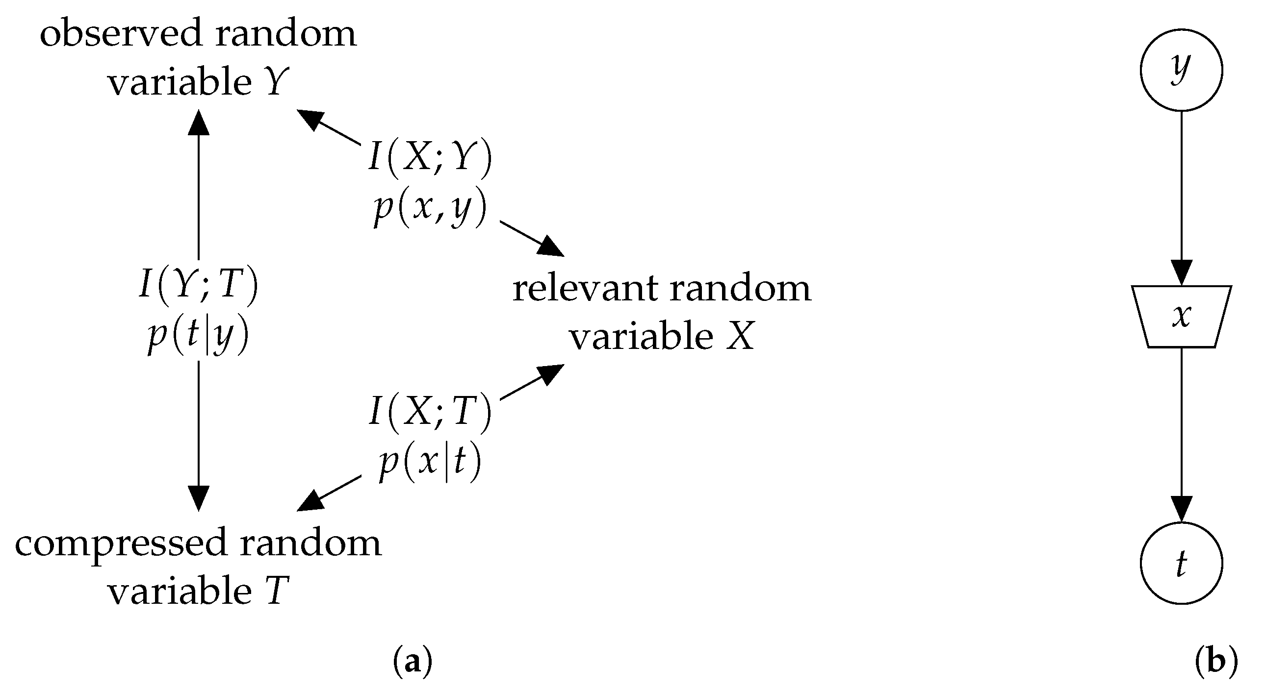
The information bottleneck method [3,4] is a generic clustering framework with its roots in the field of machine learning. Figure 3a visualizes the elementary setup of the framework. By designating a random variable X as the relevant random variable, the principal aim of the information bottleneck method is to extract as much information about X contained in an observation Y as possible and capture this relevant information in a compression variable T. More precisely, a compression mapping $p\left(t\right|y)$ is determined, which maps the event space $\mathcal{Y}$ of the observed random variable onto the event space $\mathcal{T}$ of a compression variable, such that $\left|\mathcal{T}\right|\ll \left|\mathcal{Y}\right|$ while $I(X;T)$ is maximized. In other words, the framework aims to simultaneously minimize the compression information $I(Y;T)$ and maximize the relevant information $I(X;T)$. The realizations of T are referred to as clusters whose labels can be chosen arbitrarily. We label these clusters with unsigned integer values, i.e., $\mathcal{T}=\left\{0,1,\dots ,\left|\mathcal{T}\right|-1\right\}$. The so-called information bottleneck graph [33] provides a compact visualization of this principle in Figure 3b where the observed random variable Y is compressed into T, while retaining the relevant information about X. This problem can be posed as a Lagrangian optimization problem and solved by minimizing the so-called information bottleneck functional [3]

$$\mathcal{F}\left\{p\right(t\left|y\right)\}=I(Y;T)-\beta I(X;T).$$

(13)

The non-negative Lagrangian multiplier $\beta$ in (13) serves as trade-off parameter between information preservation and compression. In extreme cases, $\beta \to \infty$ corresponds to maximum information preservation, while $\beta \to 0$ corresponds to maximum compression. In this work, we are interested in obtaining the maximum relevant information $I(X;T)$, i.e., $\beta \to \infty$. The compression results from the choice of the (constrained) cardinality of T, i.e., $\left|\mathcal{T}\right|$.

Note that after performing a mapping $p\left(t\right|y)$, any physical meaning contained in Y is lost, i.e., the compression variable T on its own has no direct meaning and belongs purely to an abstract domain. Hence, a coupling between the relevant variable X and T is needed, which is given by $p\left(x\right|t)$. Only with the distribution $p\left(x\right|t)$ can the meaning of a cluster index t for a certain x be recaptured.

Several information bottleneck algorithms exist which obtain the distributions $p\left(t\right|y)$, $p\left(x\right|t)$ and $p\left(t\right)$ from the joint distribution $p(x,y)$ [3,4]. It can be shown that choosing $\beta \to \infty$ yields a deterministic clustering $p\left(t\right|y)\in \left\{0,1\right\}$ [4]. A deterministic clustering is convenient from an implementation perspective as it can be realized as a static lookup table. An algorithm optimized for deterministic mappings that is used in this work is the modified sequential information bottleneck algorithm from [1,2], whose Python implementation is available at [34].

The information bottleneck method is a generic framework in the sense that it can be used for quantization of an observed quantity in any problem where the joint distribution $p(x,y)$ of observation y and relevant quantity x is available. With the appropriate joint distribution $p(x,y)$ at hand, the framework has been used in the field of communication for channel estimation [35], to quantize the AWGN channel and the node operations of LDPC decoders [1,2,7], the bit channels of a polar code [25], as well as the decoding operations of SC and SCL decoding of polar codes [26]. Among these applications, we explain the AWGN channel quantization using the information bottleneck framework [1,2] as an illustrative example in the following. It is important to point out that such a channel quantizer is an integral part of the information bottleneck decoders designed for LDPC and polar codes, i.e., the decoders assume that the physical channel output is clustered into a finite number of bins by a quantizer designed using the information bottleneck method or another principle.

Let $x\in \left\{0,1\right\}$ be a coded bit which is modulated into transmit symbols $s\left(x\right)$ using BPSK as $s\left(x\right)=1-2x$. The symbol $s\left(x\right)$ is affected by an AWGN with variance ${\sigma }_N^2$, resulting in continuous channel output $\tilde{y}$. Then, for the channel quantizer design using the information bottleneck, the observed and the relevant quantities are channel output $\tilde{y}$ and transmitted code bit x, respectively. The compression variable is labeled Y such that the quantized channel output is $y\in \mathcal{Y}=\left\{0,1,\dots ,\left|\mathcal{Y}\right|-1\right\}$. For the a priori distribution of $p\left(x\right)=1/2$, the joint distribution $p(x,\tilde{y})$ is given by:

$$p(x,\tilde{y})=\frac{1}{2\sqrt{2\pi {\sigma }_N^2}}exp\left(-\frac{{(\tilde{y}-s\left(x\right))}^2}{2{\sigma }_N^2}\right).$$

(14)

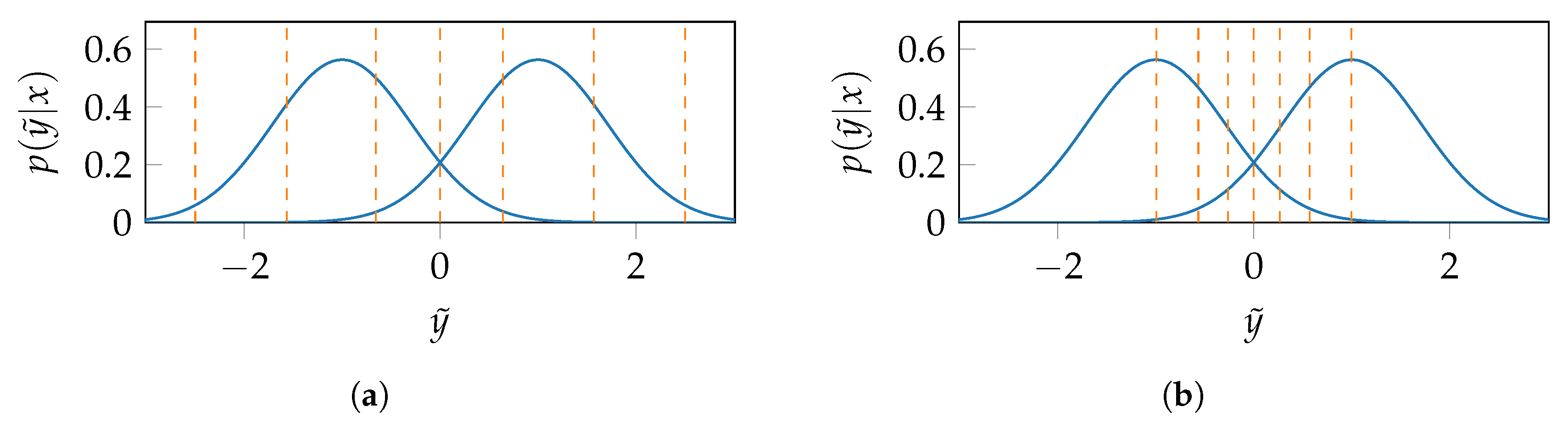
The distribution $p(\tilde{y},x)$ is fed into the modified sequential information bottleneck algorithm [1,2], which determines the mapping $p\left(y\right|\tilde{y})$ that divides the AWGN channel output into $\left|\mathcal{Y}\right|$ clusters such that $I(X;Y)$ is maximized. Note that the selected algorithm works only with discrete random variables. Therefore, the continuous channel output is first discretized using a fine uniform resolution. Figure 4 illustrates the relevant information preserving clustering of AWGN channel output into $\left|\mathcal{Y}\right|=8$ clusters for noise variance ${\sigma }_N^2=0.5$. The algorithm randomly initializes the cluster boundaries in a symmetric manner as exemplarily depicted in Figure 4a and computes the mutual information $I(X;Y)$ for the resulting compressed joint distribution $p(x,y)$. The clusters are labeled such that the left-most cluster is $y=0$, while the right-most cluster is $y=7$. When the event space $\tilde{\mathcal{Y}}$ is sorted with respect to its LLRs $2\tilde{y}/{\sigma }_N^2$, as is the case in Figure 4, each cluster is a subset of contiguous elements of $\tilde{\mathcal{Y}}$. Then, the task of finding the desired clustering $p\left(y\right|\tilde{y})$ reduces to optimizing the cluster boundaries due to the separating hyperplane condition [5]. The algorithm, therefore, adjusts each cluster boundary such that $I(X;Y)$ is maximized and updates the distributions $p(x,y)$ and $p\left(y\right|\tilde{y})$. The algorithm stops when $I(X;Y)$ does not increase further and returns the mapping $p\left(y\right|\tilde{y})$, the distribution $p\left(y\right)$, and $p\left(x\right|y)$. Figure 4b shows the optimized boundaries of quantization bins or clusters which assign all channel outputs $\tilde{y}<-0.99$ to cluster $y=0$, $-0.99\le \tilde{y}<-0.56$ to cluster $y=1$, and so on. The quantizer does not assign any real valued representative to each quantization bin but instead produces the index y of the cluster in which $\tilde{y}$ falls. Should the quantizer be used with a decoder that requires LLRs as input, the cluster indices y can be translated into channel level LLRs as:

$$\begin{array}{c}\hfill L_x^{ch}\left(y\right)=log\frac{p\left(y\right|x=0)}{p\left(y\right|x=1)}=log\frac{p(x=0|y)}{p(x=1|y)},\end{array}$$

(15)

where the distribution $p\left(x\right|y)$ is delivered by the information bottleneck algorithm along with the quantizer mapping $p\left(y\right|\tilde{y})$. The second equality in Equation (15) holds due to the equiprobable input assumption, i.e., $p\left(x\right)=0.5$.

3. Polar Code Construction Using the Information Bottleneck Method

This section describes the construction of polar codes using the information bottleneck method and compares it to the closely related construction method proposed by Tal and Vardy. Thanks to the nice recursive structure of polar codes, describing the construction steps of each method for a single building block—i.e., Figure 1—is sufficient.

3.1. Information Bottleneck Construction

The information bottleneck construction method starts by quantizing the AWGN channel using the quantizer of Section 2.4. The quantizer is designed for a target noise variance ${\sigma }_N^2$ in Equation (14), computed from the design $E_b/N_0$ of the polar code. As a result, the quantized AWGN channel becomes a binary input discrete memoryless channel with output alphabet size of $\left|\mathcal{Y}\right|$ and transition probabilities $p\left(y\right|x)$ in the building block of Figure 1. The output alphabets of the bit channels of $u_0$ and $u_1$ have sizes $|{\mathcal{Y}}_0|·|{\mathcal{Y}}_1{|=|\mathcal{Y}|}^2$ and $|{\mathcal{U}}_0|·|{\mathcal{Y}}_0|·|{\mathcal{Y}}_1{|=2·|\mathcal{Y}|}^2$, respectively. The goal here is to quantize both of the bit channels using the information bottleneck method and reduce their output alphabets to a desired size $\left|\mathcal{T}\right|$, which is chosen to be a power of 2.

Initially, the two bit channels defined over the building block of Figure 1 are casted to the information bottleneck setup of Figure 3a. For the bit channel of $u_i$, with $i\in \left\{0,1\right\}$, output ${\mathbf{y}}_i$ is the observation which we use to infer input $u_i$. Therefore, the multivariate random variable ${\mathbf{Y}}_i$ is the observed random variable, while the bit channel input is the relevant random variable, i.e., $U_i$. Our goal here is to cluster the realizations of the observed variable ${\mathbf{Y}}_i$ to a new compressed random variable $T_i=t_i\in \left\{0,1,\dots ,\left|\mathcal{T}\right|-1\right\}$, while minimizing the quantization loss in terms of mutual information $I(U_i;{\mathbf{Y}}_i)-I(U_i;T_i)$ as much as possible. The information bottleneck graphs for quantization of the two bit channels are depicted in Figure 5.

An information bottleneck algorithm requires the joint distribution $p(u_i,{\mathbf{y}}_i)$ relating the relevant and the observed random variables. For the bit channel of $u_0$, we have:

$$p(u_0,y_0,y_1)=\sum _{x_0}\sum _{x_1}\sum _{u_1}p(u_0,u_1,x_0,x_1,y_0,y_1),$$

(16)

where, from the factor graph in Figure 1:

$$\begin{array}{c}\hfill p(u_0,u_1,x_0,x_1,y_0,y_1)=p\left(y_0\right|x_0)·p\left(y_1\right|x_1)·p\left(x_0\right|u_0,u_1)·p\left(x_1\right|u_1)·p\left(u_0\right)·p\left(u_1\right).\end{array}$$

(17)

Here, $p\left(y_i\right|x_i)$ and $p\left(u_i\right)=0.5$ for $i\in \left\{0,1\right\}$ are the channel transition probabilities and priors, respectively, while $p\left(x_0\right|u_0,u_1)\in \left\{0,1\right\}$ and $p\left(x_1\right|u_1)\in \left\{0,1\right\}$ are deterministic mappings according to $x_0=u_0\oplus u_1$ and $x_1=u_1$, respectively. Applying the selected information bottleneck algorithm to the joint distribution $p(u_0,{\mathbf{y}}_0)$ will return the distributions $p\left(u_0\right|t_0)$ and $p\left(t_0\right)$, as well as the clustering $p\left(t_0\right|{\mathbf{y}}_0)$, which maps the observed sequence, ${\mathbf{y}}_0$, onto a cluster index $t_0\in \mathcal{T}$. Hence, the ${\left|\mathcal{Y}\right|}^2$ outputs of the bit channel are quantized into $\left|\mathcal{T}\right|$ clusters. The joint distribution of bit channel of $u_1$ equals:

$$p(u_1,y_0,y_1,u_0)=\sum _{x_0}\sum _{x_1}p(u_0,u_1,x_0,x_1,y_0,y_1).$$

(18)

The information bottleneck algorithm produces the distributions $p\left(u_1\right|t_1)$, $p\left(t_1\right)$ and $p\left(t_1\right|{\mathbf{y}}_1)$ for the joint distribution of Equation (18). The mapping $p\left(t_1\right|{\mathbf{y}}_1)$ clusters the $2·{\left|\mathcal{Y}\right|}^2$ outputs of the bit channel into $\left|\mathcal{T}\right|$ clusters. Thus, the output alphabet of both the bit channels is compressed to size $\left|\mathcal{T}\right|$. Further, the compressed joint distributions $p(u_i,t_i)=p\left(u_i\right|t_i)p\left(t_i\right)$ also facilitate computing the capacities of the bit channels.

For the construction of a polar code, this treatment is applied to all the building blocks in the structure of the code, starting at level $j=1$ and progressing step by step to higher levels. In our running example of Figure 2, the aforementioned procedure produces quantized bit channels at level $j=1$. Specifically, the quantized bit channels of the intermediate variables nodes labeled $v_{0,1}$ and $v_{2,1}$ are similar to the one obtained for $u_0$ of Figure 1, i.e., $p(v_{0,1},t_{0,1})=p(v_{2,1},t_{2,1})=p(u_0,t_0)$. Moreover, the quantized bit channels of the intermediate variables nodes labeled $v_{1,1}$ and $v_{3,1}$ are similar to the one obtained for $u_1$ of Figure 1, i.e., $p(v_{1,1},t_{1,1})=p(v_{3,1},t_{3,1})=p(u_1,t_1)$. At level $j=2$, the bit channel of $v_{0,2}=u_0$ now has $t_{0,1}\mathrm{and}{t}_{2,1}$ as outputs, with an output alphabet of size $|{\mathcal{T}}_{0,1}|·|{\mathcal{T}}_{2,1}{|=|\mathcal{T}|}^2$. This bit channel is quantized using the selected information bottleneck algorithm, which provides the distributions $p\left(u_0\right|t_{0,2})$, $p\left(t_{0,2}\right)$ and $p\left(t_{0,2}\right|t_{0,1},t_{2,1})$ from the input joint distribution $p(u_0,t_{0,1},t_{2,1})$, compressing the output alphabet to $\left|\mathcal{T}\right|$ elements (recall that in Figure 2, $v_{i,2}=u_i$). The input joint distribution $p(u_0,t_{0,1},t_{2,1})$ for the algorithm is computed from Equations (16) and (17) with appropriate replacements, e.g., by replacing $p\left(y_0\right|x_0)=p\left(y_1\right|x_1)$, $x_0$ and $x_1$ with $p\left(t_{0,1}\right|v_{0,1})$, $v_{0,1}$ and $v_{2,1}$, respectively. The joint distribution $p(u_1,t_{0,1},t_{2,1},u_0)$ of the bit channel of $u_1$ in Figure 2 can be obtained similarly from Equations (17) and (18) with appropriate replacements, and quantized using the information bottleneck algorithm. Figure 6 shows the resulting information bottleneck graph for the polar code of Figure 2, obtained after quantizing all the building blocks, where the output alphabet of all the bit channels is restricted to $\left|\mathcal{T}\right|$. Consequently, the compressed joint distribution $p(u_i,t_{i,2})$ for each bit channel of the code (level $j=n$) can be used to compute its capacity using Equation (12), and thus to construct information set $\mathcal{A}$ [25].

3.2. Tal and Vardy’s Construction

The key step of Tal and Vardy’s construction method is the degrading procedure which merges the elements in the output alphabet of a binary input discrete memoryless symmetric channel. Assume that the output alphabet $\mathcal{Y}$ of the channel characterized by $p\left(y\right|x)$ in Figure 1 has $\left|\mathcal{Y}\right|$ elements which we wish to reduce to $\left|\mathcal{T}\right|<\left|\mathcal{Y}\right|$. The target alphabet size $\left|\mathcal{T}\right|$ is referred to as the fidelity parameter in [23] and denoted by $\mu$. The output alphabet size is reduced by one, if two elements $y_a,y_b\in \mathcal{Y}$ are merged into a single element $y_{ab}$. The output alphabet becomes $\mathcal{Y}\backslash \left\{y_a,y_b\right\}\cup \left\{y_{ab}\right\}$, and the transition probabilities are updated as:

$$p\left(y\right|x)=\left\{\begin{array}{cc}p\left(y_a\right|x)+p\left(y_b\right|x)\hfill & y=y_{ab}\hfill \\ p\left(y\right|x)\hfill & \mathrm{otherwise}.\hfill \end{array}\right.$$

(19)

Such a merging always causes a loss in the capacity of the channel amounting to $\delta I\ge 0$. Tal and Vardy’s degrading merge procedure chooses the elements to be merged wisely; the pair of elements to be merged is selected such that their merging will cause the smallest amount of loss $\delta I$. Such a degrading merge is performed repeatedly, until the output alphabet size of the channel is reduced to the desired value of $\left|\mathcal{T}\right|$. The bit channels synthesized from such a channel using Equations (2) and (3) will have an output alphabet size of ${\left|\mathcal{T}\right|}^2$ and ${2\left|\mathcal{T}\right|}^2$, respectively. The aforementioned degrading merge is applied to each bit channel such that their output alphabet sizes are reduced to $\left|\mathcal{T}\right|$. For constructing a polar code with $N>2$, the degrading merge is used after application of the polarization transform at each level, and the output alphabet size of the (intermediate) bit channels is kept restricted to $\left|\mathcal{T}\right|$. Equation (11) is then used to compute the error probability of each degraded bit channel, which serves as an upper bound on the error probability of the unquantized bit channel.

Tal and Vardy performed the degrading merge in an efficient way by exploiting the symmetry of the channel. Firstly, the elements of $\mathcal{Y}$ are sorted with respect to their LLRs. In the sorted output alphabet, only pairs of consecutive elements need to be considered for merging ([23], Theorem 8). Secondly, due to the channel symmetry, for each $y\in \mathcal{Y}$ there exists a $\overline{y}\in \mathcal{Y}$, referred to as the conjugate of y, such that $p\left(y\right|x=0)=p\left(\overline{y}\right|x=1)$. This fact is exploited in the sense that computations for mergers are done for half of the channel output alphabet ${\mathcal{Y}}^{+}$, where:

$$\begin{array}{c}\hfill {\mathcal{Y}}^{+}=\left\{y\in \mathcal{Y}:logp\left(y\right|x=0)/p(y|x=1)>0\right\}.\end{array}$$

When a pair $y_a,y_b\in {\mathcal{Y}}^{+}$ is merged into $y_{ab}$, their conjugates ${\overline{y}}_a,{\overline{y}}_b\in \mathcal{Y}\backslash {\mathcal{Y}}^{+}$ are also merged into ${\overline{y}}_{ab}$.

The final code construction algorithm computes the upper bounds on the error probabilities of the bit channels using the degrading merge procedure and also computes the Bhattacharyya parameter for each bit channel. The smallest of the two is then considered for including a bit channel into information set $\mathcal{A}$. In order to track the inaccuracy introduced by the quantization, another approximation, namely, the upgrading merge is used. For every bit channel which is quantized using the degrading merge, the upgrading merge synthesizes another bit channel, with alphabet size $\left|\mathcal{T}\right|$, which is upgraded, i.e., its probability of error is equal or smaller than that of the channel under consideration. The error probability of the upgraded channel provides a lower bound on the probability of error of a bit channel. The value of $\left|\mathcal{T}\right|$ is then selected such that the two bounds are very close to each other. When such a value for $\left|\mathcal{T}\right|$ is found, the upgrading merge can be discarded. $\left|\mathcal{T}\right|=256$ or 512 was shown to suffice ([23], Figure 2 and Table I).

For the binary input AWGN channel $p\left(\tilde{y}\right|x)$, the continuous output $\tilde{y}$ is first descritized into a fine resolution with $|{\mathcal{T}}_{ch}|\gg |\mathcal{T}|$. However, the bit channels synthesized from this fine resolution quantized channel have their output alphabets reduced to $\left|\mathcal{T}\right|$ using the aforementioned degrading merge procedure. Therefore, the code construction at higher levels $j>1$ in the code structure for $N>2$ procedes as explained for channels with discrete output.

3.3. Information Bottleneck vs. Tal and Vardy Construction

In this section, polar code construction using the information bottleneck method and the Tal and Vardy method are compared. The working principle behind both construction methods is the same: Compress the output alphabet of bit channels at each level j while keeping the loss of mutual information caused by the compression as small as possible. In fact, the degrading merge procedure of Tal and Vardy’s construction ([23] Algorithm C) is known as the modified agglomerative information bottleneck algorithm in the information bottleneck circle [36]. However, since Tal and Vardy’s construction method also uses the Bhattacharyya parameter for designating a bit channel to be frozen or not, it is a fusion of the information bottleneck method and Arikan’s approximation [13]. Some further differences between the two methods are as follows.

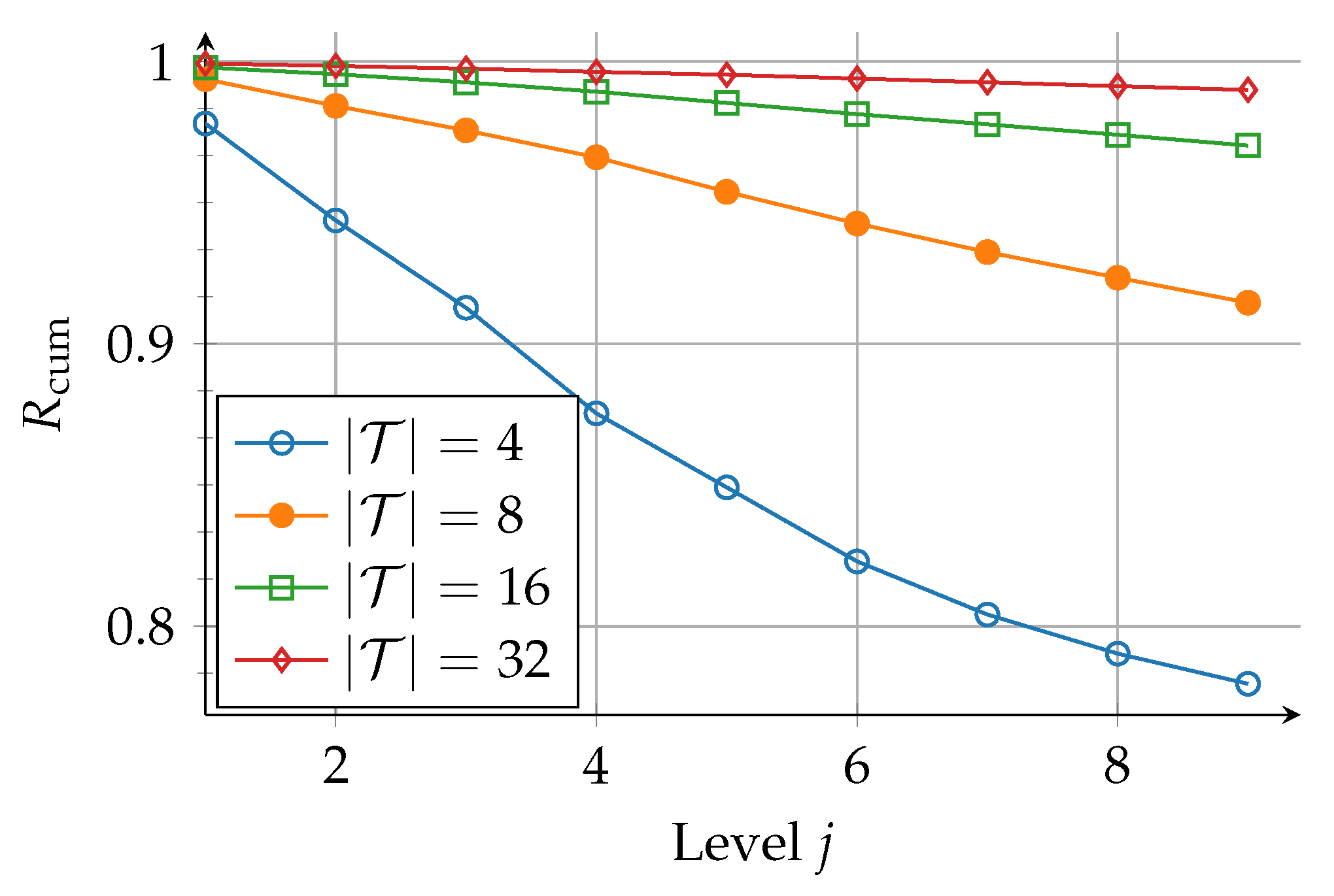
The rule used to choose the quantized alphabet size $\left|\mathcal{T}\right|$ in Tal and Vardy’s method is different than that used in the information bottleneck method. Tal and Vardy’s method chooses $\left|\mathcal{T}\right|$ such that the bounds obtained from degrading and upgrading merge are very close, and thus, the values $\left|\mathcal{T}\right|=256$ or 512 are suggested. On the other hand, the choice of $\left|\mathcal{T}\right|$ in the information bottleneck method is driven by tracking the amount of relevant mutual information retained during the density evolution across the levels of a polar code. For that purpose, the rate of preserved mutual information for quantizing the ith (intermediate) bit channel at a level j is defined as $R_{i,j}=I(V_{i,j};T_{i,j})/I(V_{i,j};{\mathbf{Y}}_{i,j})$, where $I(V_{i,j};T_{i,j})$ is the preserved mutual information after compression and $I(V_{i,j};{\mathbf{Y}}_{i,j})$ is the mutual information before the compression. Then, the rate of mutual information preservation $R_j$ for the jth level is defined as the mean of the $R_{i,j}$ values. For a codeword length of $N=2^n$, the overall rate of information preservation is computed as a cumulative product, $R_{cum}$:

$$R_{cum}=R_1\times R_2\times \cdots \times R_n.$$

(20)

Figure 7 shows the evolution of $R_{cum}$ over the levels in the polar code structure for different compressed cardinalities $\left|\mathcal{T}\right|$. Considering a polar code with length $N=512$, already for a quite small number of 16 clusters, approximately $98\%$ of relevant information is preserved over all levels. Increasing the number of clusters further to 32 yields only a small gain, i.e., $99\%$ of relevant information is preserved. Hence, the information bottleneck construction method is computationally more efficient than Tal and Vardy’s method due to the use of small values of $\left|\mathcal{T}\right|$.

The information bottleneck construction method benefits from the availability of different algorithms and hence offers to choose an algorithm according to the problem at hand, e.g., an information bottleneck algorithm with a nonbinary relevant variable can be chosen for constructing nonbinary polar codes. Another difference between the two construction methods is that while Tal and Vardy’s method incorporates the channel quantizer into the merging operations at level $j=1$, the information bottleneck method separates the channel quantizer design from the code structure. This adds flexibility to the information bottleneck construction method and facilitates construction of polar codes for other channel models or modulation schemes. For instance, replacing the channel quantizer of Section 2.4 with the one from [37], i.e., designed using the information bottleneck method for an AWGN channel with 16-QAM input symbols, the construction method can be adapted for constructing a polar codes for a higher order modulation scheme.

Lastly, the Tal and Vardy method does not fully exploit the benefits of the discrete density evolution performed for code construction, i.e., the intermediate results could be used for decoding. The benefits of application of the information bottleneck method in polar codes go beyond the code construction. For each variable node $v_{i,j}$, $0\le i<N$ and $1\le j\le n$, in Figure 2, the distributions $p\left(t_{i,j}\right|{\mathbf{y}}_{i,j})$ and $p\left(v_{i,j}\right|t_{i,j})$ are obtained. Here, ${\mathbf{y}}_{i,j}$ represents the output of the virtual bit channel experienced by $v_{i,j}$, and $t_{i,j}$ is the cluster index in which ${\mathbf{y}}_{i,j}$ falls. With appropriate book keeping, we save all the hard work done during the discrete density evolution for computing these distributions and use them for coarsely quantized decoding as shown in the next section.

4. Information Bottleneck Polar Decoders

In this section, we show how the results of polar code construction using the information bottleneck method can also be used for coarsely quantized SC and SCL decoding [26]. Note that the lookup tables used for decoding in the following section are generated offline for a single design $E_b/N_0$ and are used mismatched to the whole operating $E_b/N_0$ range. First, decoding at a single building block is demonstrated, followed by demonstration of SCL decoding in Figure 2.

4.1. Lookup Tables for Decoding on a Building Block

In Section 3.1, the distributions $p\left(t_i\right|{\mathbf{y}}_i)$ and $p\left(u_i\right|t_i)$, $i\in \left\{0,1\right\}$, were obtained from $p(u_i,{\mathbf{y}}_i)$ using the information bottleneck method on the building block of Figure 1. The joint distribution, $p(u_i,{\mathbf{y}}_i)$, of a bit channel embeds the relation of its output ${\mathbf{y}}_i$ to its input $u_i$, i.e., knowing ${\mathbf{y}}_i$, one can figure out whether $u_i=0$ or $u_i=1$ is more probable. By ensuring that $I(U_i;T_i)\approx I(U_i;{\mathbf{Y}}_i)$, the information bottleneck method strives to preserve this relation when compressing and mapping the event space of ${\mathbf{Y}}_i$ onto that of $T_i$. Therefore, knowing the value of $T_i=t_i$ (i.e., the label of the cluster to which the channel output belongs) after using the mapping $p\left(t_i\right|{\mathbf{y}}_i)$, we can figure out the most likely value of the channel input.

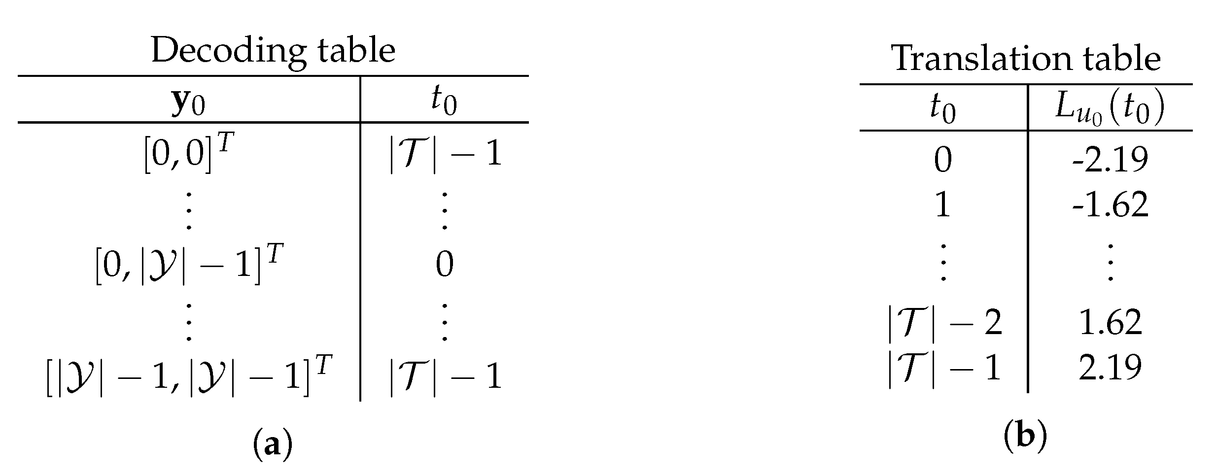
The deterministic mapping $p\left(t_i\right|{\mathbf{y}}_i)$ in tabular form is referred to as the decoding table for the bit $u_i$, e.g., Figure 8a shows the decoding table for $u_0$. The decoding table of $u_0$ is essentially a quantizer of the bit channel $p(y_0,y_1|u_0)$ which produces the cluster index $t_0\in \mathcal{T}$ when the outputs of the underlying AWGN channel are put in clusters $y_0$ and $y_1$ by the channel quantizer. Typically, the cluster index alone does not provide any meaning for the relevant quantity. However, due to the symmetry of the bit channel, the knowledge of $t_0$ can be used for a hard decision on $u_0$ since half of the $\left|\mathcal{T}\right|$ clusters correspond to $u_0=0$ and the remaining half to $u_0=1$. In order to perform soft decision estimation, the conditional distribution $p\left(u_0\right|t_0)$ is used to compute the LLR $L_{u_0}\left(t_0\right)$ as:

$$L_{u_0}\left(t_0\right)=log\frac{p\left(t_0\right|u_0=0)}{p\left(t_0\right|u_0=1)}=log\frac{p(u_0=0|t_0)}{p(u_0=1|t_0)},$$

(21)

where the second equality in Equation (21) is due to equiprobable input, i.e., $p\left(u_0\right)=0.5$. Equation (21) is tabulated with exemplary values in Figure 8b and referred to as the translation table since it translates the cluster indices $t_0\in \{0,1,\dots ,|\mathcal{T}|-1\}$ to LLRs $L_{u_0}\left(t_0\right)$. It can be seen in the translation table of Figure 8b that ${\widehat{u}}_0=1$ is most likely for all the bit channel outputs ${\mathbf{y}}_0$ put in the cluster $t_0=0$, i.e., the largest LLR magnitude with a negative sign. When the decoding table lookup produces $t_0=1$, ${\widehat{u}}_0=1$ is still more probable but with less confidence, i.e., smaller LLR magnitude. The lookup tables of Figure 8 can be used to decode $u_0$ as follows:

• Use the decoding table $p\left(t_0\right|{\mathbf{y}}_0)$ of Figure 8a to determine the cluster index to which the observed channel output ${\mathbf{y}}_0$ belongs. For example, $t_0=\left|\mathcal{T}\right|-1$ when $y_0=y_1=0$.
• Use $t_0$ from step 1 for a hard decision on $u_0$ or translate it into an LLR value using the translation table of Figure 8b. For the example of $t_0=\left|\mathcal{T}\right|-1$, ${\widehat{u}}_0=0$ and $L_{u_0}\left(t_0\right)$$=2.19$.

The bit $u_1$ can also be decoded in a similar fashion using its decoding and translation tables $p\left(t_1\right|{\mathbf{y}}_1)$ and $p\left(u_1\right|t_1)$, respectively. Similarly to conventional SC decoding, the decoding table of $u_1$ assumes the knowledge of $u_0$ from the previous decoding stage. Thus, the decoding on a building block can be done using lookup tables instead of computations according to Equations (6a) and (6b). The decoding tables $p\left(t_0\right|{\mathbf{y}}_0)$ and $p\left(t_1\right|{\mathbf{y}}_1)$ have ${\left|\mathcal{Y}\right|}^2$ and $2·{\left|\mathcal{Y}\right|}^2$ integer valued entries, respectively. Both the translation tables have only $\left|\mathcal{T}\right|$ real valued entries, i.e., LLRs.

4.2. Information Bottleneck Successive Cancellation List Decoder

Having replaced the decoding steps on a single building block with table lookups, we proceed to demonstrate successive cancellation list decoding on the code of Figure 2 using lookup tables. For each variable node $v_{i,j}$, $0\le i<N$ and $1\le j\le n$, in Figure 2, the decoding table $p\left(t_{i,j}\right|{\mathbf{y}}_{i,j})$ and the translation table $p\left(v_{i,j}\right|t_{i,j})$ is available from application of the information bottleneck framework to the whole structure of Figure 2. Assume that the decoding list size is $N_L=2$ and $\mathcal{A}=\left\{1,2,3\right\}$, i.e., only $u_0=0$ is frozen.

With the right-most variable nodes, i.e., $v_{i,0}$ loaded with quantizer output $y_i$, $i=0,1,2,3$, the decoding starts with the frozen bit $u_0$. Although the value of $u_0$ is known, its LLR $L_{u_0}\left(t_0\right)$ is required for the path metric update according to Equation (9). Therefore, cluster index $t_{0,2}$ needs to be known from the decoding table $p\left(t_{0,2}\right|{\mathbf{y}}_{0,2})=p\left(t_{0,2}\right|t_{0,1},t_{2,1})$. In order to obtain the yet unknown cluster values $t_{0,1}$ and $t_{2,1}$, the decoding tables $p\left(t_{0,1}\right|{\mathbf{y}}_{0,1})=p\left(t_{0,1}\right|y_0,y_1)$ and $p\left(t_{2,1}\right|{\mathbf{y}}_{2,1})=p\left(t_{2,1}\right|y_2,y_3)$ are used, respectively. Once the cluster values $t_{0,1}$ and $t_{2,1}$ are obtained, the decoding table $p\left(t_{0,2}\right|{\mathbf{y}}_{0,2})$ is used to get the value of $t_{0,2}$. The translation table $p\left(u_0\right|t_{0,2})$ is used to translate $t_{0,2}$ to LLR $L_{u_0}\left(t_0\right)$, which is used to update path metric $M_{0,0}$.

In the next decoding stage, the first information bit $u_1$ is decoded. The cluster index $t_{1,2}$ is obtained from the decoding table $p\left(t_{1,2}\right|{\mathbf{y}}_{1,2})=p\left(t_{1,2}\right|t_{0,1},t_{2,1},u_0)$, for which all the three inputs are known from the previous decoding stage. The translation table $p\left(u_1\right|t_{1,2})$ is used to translate $t_{1,2}$ to LLR $L_{u_1}\left(t_1\right)$. Instead of using Equation (5) for the information bit, the decoder extends the existing decoding path with both possible decisions ${\widehat{u}}_1=0$ and ${\widehat{u}}_1=1$ and updates the path metrics $M_{1,l}$, $l\in \left\{0,1\right\}$ for both paths using $L_{u_1}\left(t_1\right)$ in (9). Similar steps are taken to estimate the remaining bits, i.e., $u_2$ and $u_3$. At each decoding stage $i\in \mathcal{A}$, the number of decoding paths in the list doubles, and for $i\ge 2$, the decoding list size will exceed the maximum allowed value $N_L=2$. Therefore, $N_L$ of the decoding paths having the largest path metric are dropped from the decoding list.

The schedule of computations in the lookup table-based decoder is the same as in a conventional SCL decoder. However, all the computations, except the path metric update, are replaced by table lookups. Further, the inputs and outputs of all the decoding tables are unsigned integers, i.e., $0,1,\dots ,\left|\mathcal{T}\right|-1$ with $\left|\mathcal{T}\right|$ being a small number. The translation tables hold LLR values, i.e., real numbers. For a polar code of length N, $2N-2$ distinct decoding tables are required. It is important to note that the translation tables are required only at the decision level, i.e., $j=n$, in the information bottleneck SCL decoders when an LLR value is needed for Equation (9). Therefore, we require only N translation tables. Moreover, at any level j, every decoding table at an even stage i requires ${\left|\mathcal{T}\right|}^2·Q_t$ bits of memory, while each decoding table at an odd stage i requires $2·{\left|\mathcal{T}\right|}^2·Q_t$ bits of memory, where $Q_t={log}_2\left|\mathcal{T}\right|$ is the number of bits required to represent a cluster index $t_{i,j}$. If the LLR values in the translation tables are stored using a resolution of $Q_{LLR}$ bits, the N translation tables will consume a memory of $N·\left|\mathcal{T}\right|·Q_{LLR}$ bits.

5. Space-Efficient Information Bottleneck Successive Cancellation List Decoder

The computational simplicity of the information bottleneck SCL decoding comes at the cost of additional memory for storing the decoding and translation tables. In this section, we show how to reduce the memory requirement of the translation tables in an information bottleneck SCL decoder. First, the role of translation tables is discussed in detail. Then, the message alignment principle of [7] is exploited to obtain a single translation table that can be used instead of the N distinct translation tables. For the following discussion, we drop the level subscript from cluster indices at the nth level for the sake of brevity and write $t_{i,n}$ as $t_i$.

5.1. The Role of Translation Tables

The output of all the decoding table lookups in the structure of an information bottleneck SCL decoder has the same alphabet $t_{i,j}\in \left\{0,1,\dots ,\left|\mathcal{T}\right|-1\right\}$. The purpose of translation tables is to decipher the cluster index $t_i$, an abstract quantity obtained from a decoding table lookup, at the decision level into LLR $L_{u_i}\left(t_i\right)$, i.e., its meaning for the bit $u_i$. The reason for requiring a distinct translation table for each bit lies in the fact that the translation tables of two qualitatively different bit channels translate the same cluster index into an LLR value differently. Figure 9 shows the translation tables for bits $u_{14},u_{83}$, and $u_{124}$ of an information bottleneck SCL decoder with $\left|\mathcal{T}\right|=16$ generated for a half-rate polar code with $N=128$ and design $E_b/N_0=3$ dB. In the figure, cluster indices are given along the x-axis, while the LLR values they correspond to are given along the y-axis. It can be seen that $L_{u_{14}}\left(t_{14}\right)\ne L_{u_{83}}\left(t_{83}\right)\ne L_{u_{124}}\left(t_{124}\right)$ if $t_{14},t_{83}$, and $t_{124}$ take the same numerical value, e.g., $t_{14}=t_{83}=t_{124}=0$. Further, the same cluster index translates to different LLR magnitudes not only for frozen and information bits, but also for different information bits. However, one notices that $L_{u_{14}}\left(t_{14}\right)\ne L_{u_{83}}\left(t_{83}\right)$ for $t_{14}=1$ and $t_{83}=5$. Similarly, $L_{u_{14}}\left(t_{14}\right)\ne L_{u_{124}}\left(t_{124}\right)$ for $t_{14}=2$ and $t_{124}=7$. We need to somehow align all the translation tables such that a cluster index t translates to the same LLR value regardless of the bit channel i, $0\le i<N$, for which it is used.

5.2. Message Alignment for Successive Cancellation List Decoder

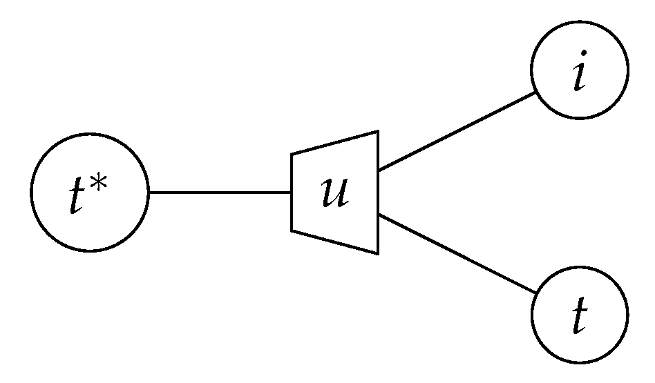
Recall that the cluster indices $t_i$ take values from the same finite alphabet $\mathcal{T}=\left\{0,1,\dots ,\left|\mathcal{T}\right|-1\right\}$ regardless of the decoding stage i, e.g., we can have $t_{14}=1$ and $t_{83}=1$. However, the appropriate translation table, obtained from the conditional distribution $p\left(u_i\right|t_i)$ according to Equation (21), translates the cluster index $t_i$ into an LLR $L_{u_i}\left(t_i\right)$. Now let us make some notational changes. We separate the stage subscript from the cluster index and express $t_i$ as a pair ${[t,i]}^T$. In our new notation, $t_{14}=1$ and $t_{83}=1$ are expressed as ${[1,14]}^T$ and ${[1,83]}^T$, respectively. We drop the subscript i from the bit $u_i$ altogether such that a bit value is denoted by u regardless of the decoding stage i. Thus, the use of distinct translation tables with this new notation can be stated as follows; a correct translation of a cluster index $t\in \left\{0,1,\dots ,\left|\mathcal{T}\right|-1\right\}$ into an LLR $L_u\left(t\right)$ requires the knowledge of the decoding stage $i\in \left\{0,1,\dots ,N-1\right\}$. In other words, we observe t and i and infer the value of bit u. This task of message alignment can be treated as an information bottleneck problem; the pair ${\mathbf{y}}^{\ast }={[t,i]}^T$ is the observed quantity, while the bit u is the relevant quantity, depicted in the information bottleneck graph of Figure 10. Casting the problem to the setup of Figure 3a, U becomes the binary relevant random variable, while ${\mathit{Y}}^{\ast }$ is the observed random variable with $|{\mathcal{Y}}^{\ast }|=N·|\mathcal{T}|$. We wish to compress ${\mathit{Y}}^{\ast }$ into a new variable $T^{\ast }$ with realizations $t^{\ast }\in {\mathcal{T}}^{\ast }=\left\{0,1,\dots ,|{\mathcal{T}}^{\ast }|-1\right\}$ such that $I(U;T^{\ast })$ is maximized. We refer to $|{\mathcal{T}}^{\ast }|$ as the alignment cardinality.

The application of an information bottleneck algorithm requires the joint distribution of the observation and the relevant quantity, i.e., $p(u,{\mathbf{y}}^{\ast })$. This joint distribution is given by:

$$p(u,{\mathbf{y}}^{\ast })=p(u,t,i)=p\left(i\right)p(u,t|i)=\frac{1}{N}p(u_i,t_i),$$

(22)

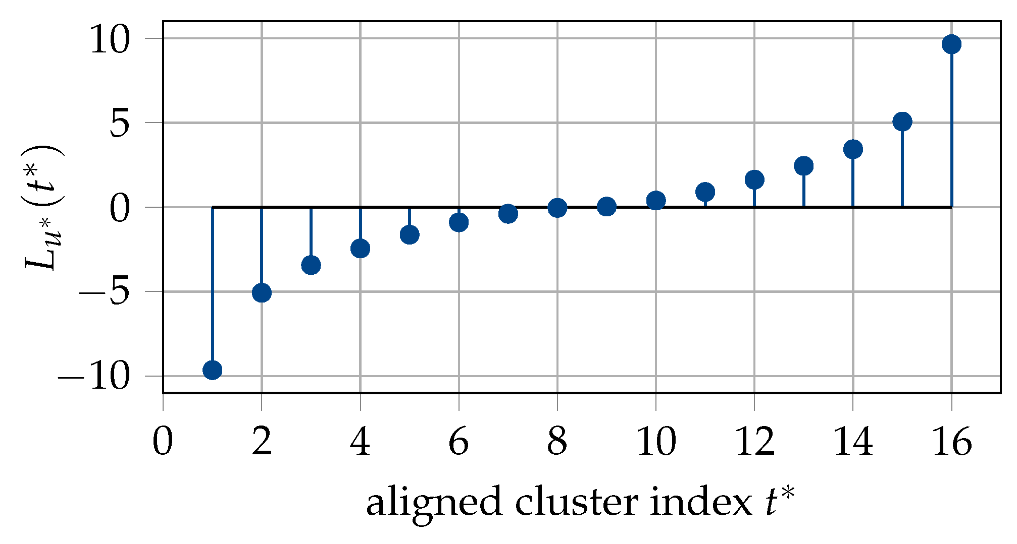
where $p(u_i,t_i)$ is available from the information bottleneck decoder construction via density evolution and $p\left(i\right)=\frac{1}{N}$ since there are N translation tables, each occurring once. The algorithm returns the distributions $p\left(u\right|t^{\ast })$ and $p\left(t^{\ast }\right)$, as well as the mapping $p\left(t^{\ast }\right|{\mathbf{y}}^{\ast })$, which clusters the pairs ${[t,i]}^T$ to $t^{\ast }$. The alignment mapping $p\left(t^{\ast }\right|{\mathbf{y}}^{\ast })$ needs not to be implemented as an extra table lookup and can be incorporated in the decoding tables at the $j=n$ level. The mapping $p\left(t^{\ast }\right|{\mathbf{y}}^{\ast })$ is used to replace the cluster indices ${\mathbf{y}}^{\ast }={[t,i]}^T=t_i$ in the decoding tables of the decision level, i.e., $p\left(t_i\right|{\mathbf{y}}_{i,n})$, with the cluster indices $t^{\ast }$. In other words, the decoding tables at the decision level are aligned. As a result, the aligned cluster indices $t^{\ast }$ are translated using a single new translation table obtained from $p\left(u\right|t^{\ast })$ in line with Equation (21). Figure 11 depicts the aligned translation table for the polar code of Section 5.1 obtained for $|{\mathcal{T}}^{\ast }|=16$.

It is pointed out that we are free to choose the alignment cardinality $|{\mathcal{T}}^{\ast }|$. The choice of $|{\mathcal{T}}^{\ast }|$, however, affects the performance of the quantized decoders, as seen in the next section. Moreover, the aligned decoding tables at the decision level require a memory of ${\left|\mathcal{T}\right|}^2·Q_{t^{\ast }}$ or $2·{\left|\mathcal{T}\right|}^2·Q_{t^{\ast }}$ bits instead of ${\left|\mathcal{T}\right|}^2·Q_t$ or $2·{\left|\mathcal{T}\right|}^2·Q_t$ bits, respectively, where $Q_{t^{\ast }}={log}_2\left|{\mathcal{T}}^{\ast }\right|$. Therefore, when $|{\mathcal{T}}^{\ast }|$ is chosen to be larger than $\left|\mathcal{T}\right|$, the size, i.e., the number of elements in each decoding table at the decision level remains unchanged, but the memory required for each decoding table increases since $Q_{t^{\ast }}>Q_t$.

6. Numerical Results

This section provides a comparison of the information bottleneck and Tal and Vardy code construction and discussion of the simulation results for the information bottleneck decoders.

6.1. Code Construction

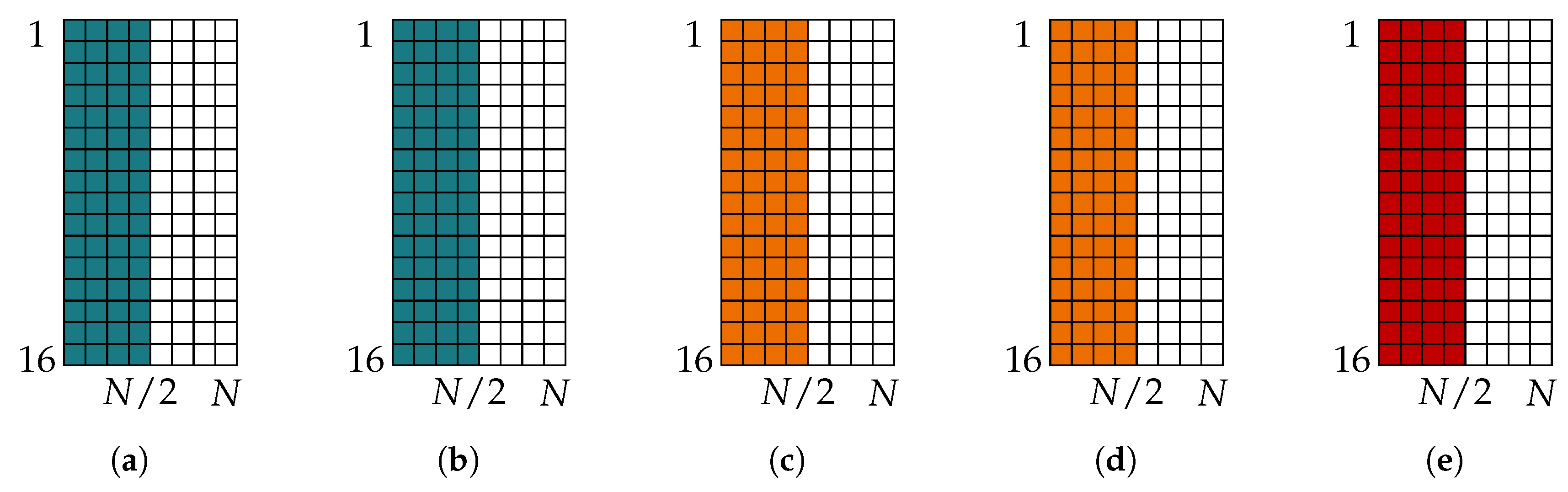
Figure 12 and Figure 13 present the so-called frozen charts, a compact visualization of information sets from [38], for polar codes constructed using Tal and Vardy’s method and the information bottleneck method, as well as the Gaussian approximation [24]. A frozen chart is a grid of squares where each square denotes a bit channel, starting from top left and reading columnwise. A colored square denotes a frozen bit position, while a white square represents an information bit position. The bit channels in the frozen charts are sorted with respect to the descending order of their error probabilities obtained from Tal and Vardy’s method with $\left|\mathcal{T}\right|=512$ such that the top left square represents the least reliable bit channel, while the bottom right square represents the most reliable bit channel. Each polar code is constructed for rate 0.5 such that $K=N/2$ worst bit channels are frozen. The design $E_b/N_0$ for any polar code presented in this paper is selected in the following way. First, the block error probability of the code with target code rate and codeword length N is computed using Equation (3) from [39] for various candidate $E_b/N_0$ values. Then, the candidate value which achieves the block error probability of ${10}^{-3}$ at the smallest $E_b/N_0$ is selected as the design $E_b/N_0$ for the polar code.

Figure 12 shows the frozen charts obtained for $N=128$. It is seen that the codes obtained from all of the construction methods are the same. Especially, Tal and Vardy polar codes for $\left|\mathcal{T}\right|=512$ and $\left|\mathcal{T}\right|=16$ are the same. This result suggests that although the bounds on the error probability of the bit channels from Tal and Vardy’s method might not be tight with $\left|\mathcal{T}\right|=16$, the resulting information set is the same as the one obtained for $\left|\mathcal{T}\right|=512$. The frozen charts of the codes constructed using the information bottleneck method for $\left|\mathcal{T}\right|=16$ and $\left|\mathcal{T}\right|=32$ are also the same. Hence, for a given code rate and design $E_b/N_0$, all the methods compared here produce the same information sets, regardless of the choice of $\left|\mathcal{T}\right|$.

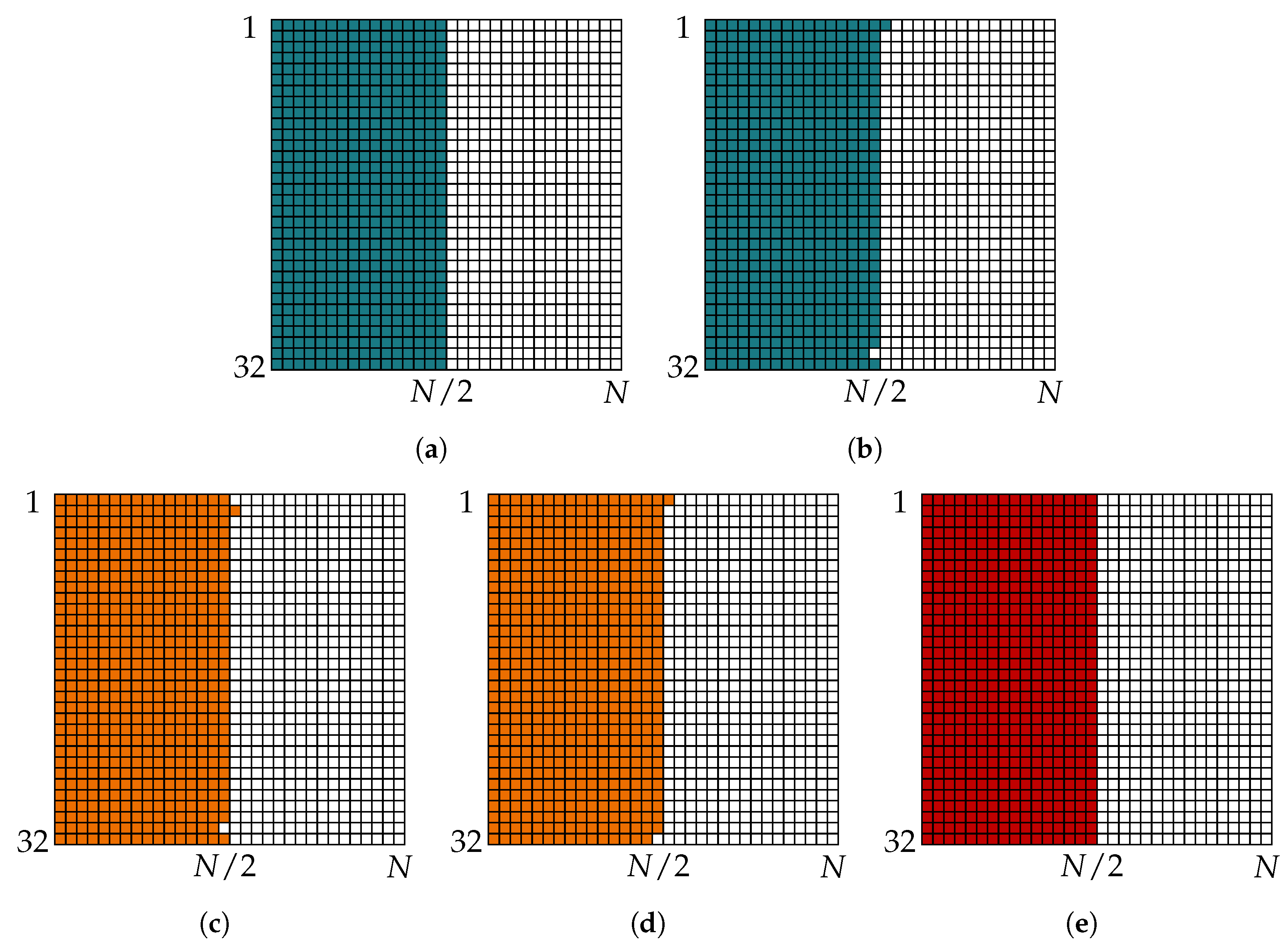
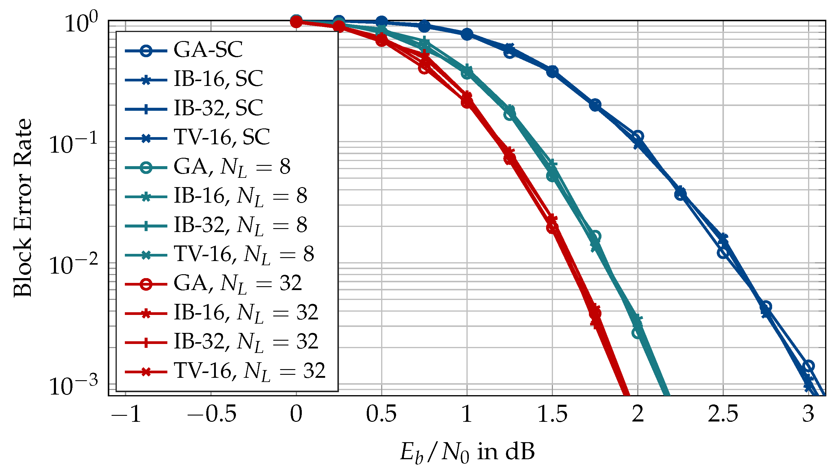
Figure 13 shows the frozen charts obtained for $N=1024$. It is seen that the codes obtained from various construction methods are slightly different for the larger codeword length. Tal and Vardy polar codes for $\left|\mathcal{T}\right|=512$ and $\left|\mathcal{T}\right|=16$ differ in a few positions (cf. Figure 13a,b). The same is true for codes constructed with the information bottleneck method (cf. Figure 13c,d). Interestingly, the codes constructed using Tal and Vardy’s method with $\left|\mathcal{T}\right|=512$ in Figure 13a are exactly the same as the ones constructed using the Gaussian approximation (cf. Figure 13e) and differ from the frozen chart of the information bottleneck polar code of Figure 13d in only two positions. Hence, the codes constructed for coarsely quantized decoders do not differ significantly from those designed for high-resolution decoding. The important question here is how much such small differences affect the error correction performance of the polar code. Figure 14 shows the block error rate of using the information sets of Figure 13. It is obvious from Figure 14 that the minor differences in the information sets obtained from various construction methods and different quantization parameters $\left|\mathcal{T}\right|$ have a negligible effect on the block error rates of polar code under SC decoding and CRC-aided SCL decoding with different list sizes. Hence, we are encouraged to consider the code and the decoder design separately and choose the least computationally intensive code construction method, i.e., the Gaussian approximation.

6.2. Information Bottleneck Decoders

In this section, the simulation results on the error correction performance of the coarsely quantized information bottleneck decoders are discussed. In all the simulations in the following discussion, an AWGN channel with BPSK modulation is assumed. The information bottleneck decoders and the information bottleneck quantizer have the same resolution, i.e., $\left|\mathcal{Y}\right|=\left|\mathcal{T}\right|$. The conventional SCL decoders use double-precision, floating-point arithmetic, i.e., they assume virtually no quantization and have a 64-bit resolution. The CRC-aided settings are used where a value for $N_{crc}$ is specified. It should be pointed out that we did not attempt to optimize the design $E_b/N_0$ over the error rate of the information bottleneck decoders in this work. The design $E_b/N_0$ is selected as mentioned in Section 6.1 to obtain the information set $\mathcal{A}$ of a polar code. Then, the error correction performance of a conventional SCL (SC) decoder is compared to that of an information bottleneck SCL (SC) decoder generated for that design $E_b/N_0$.

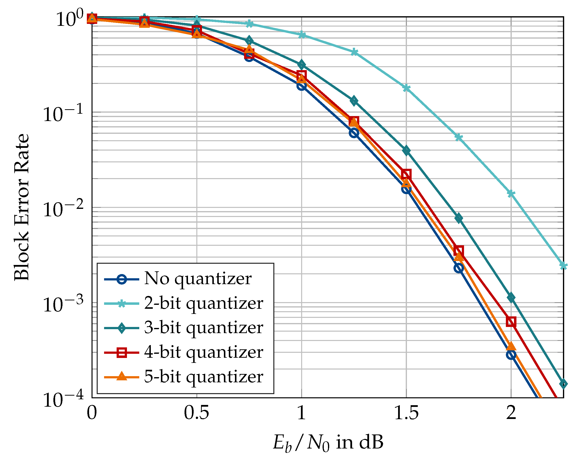
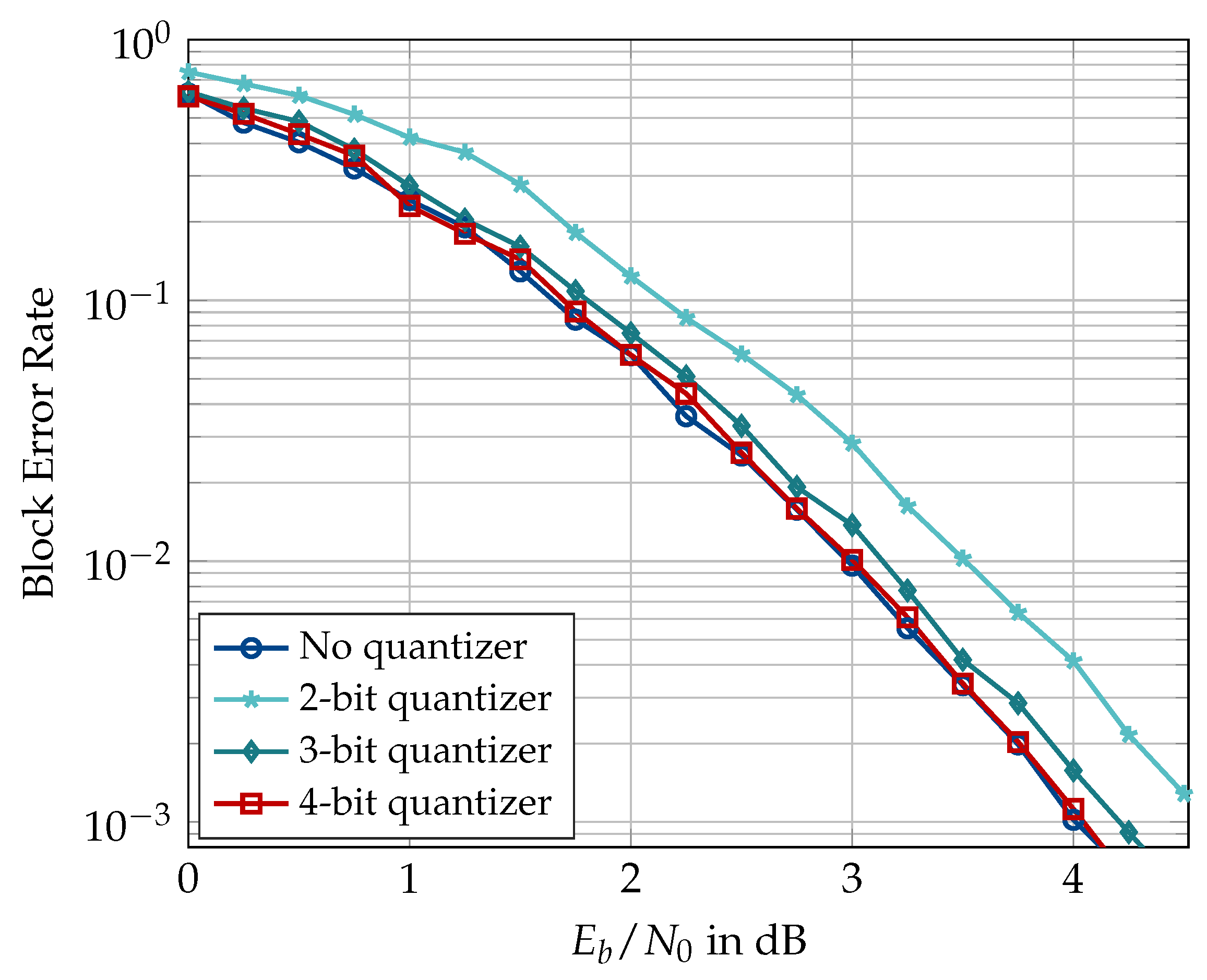
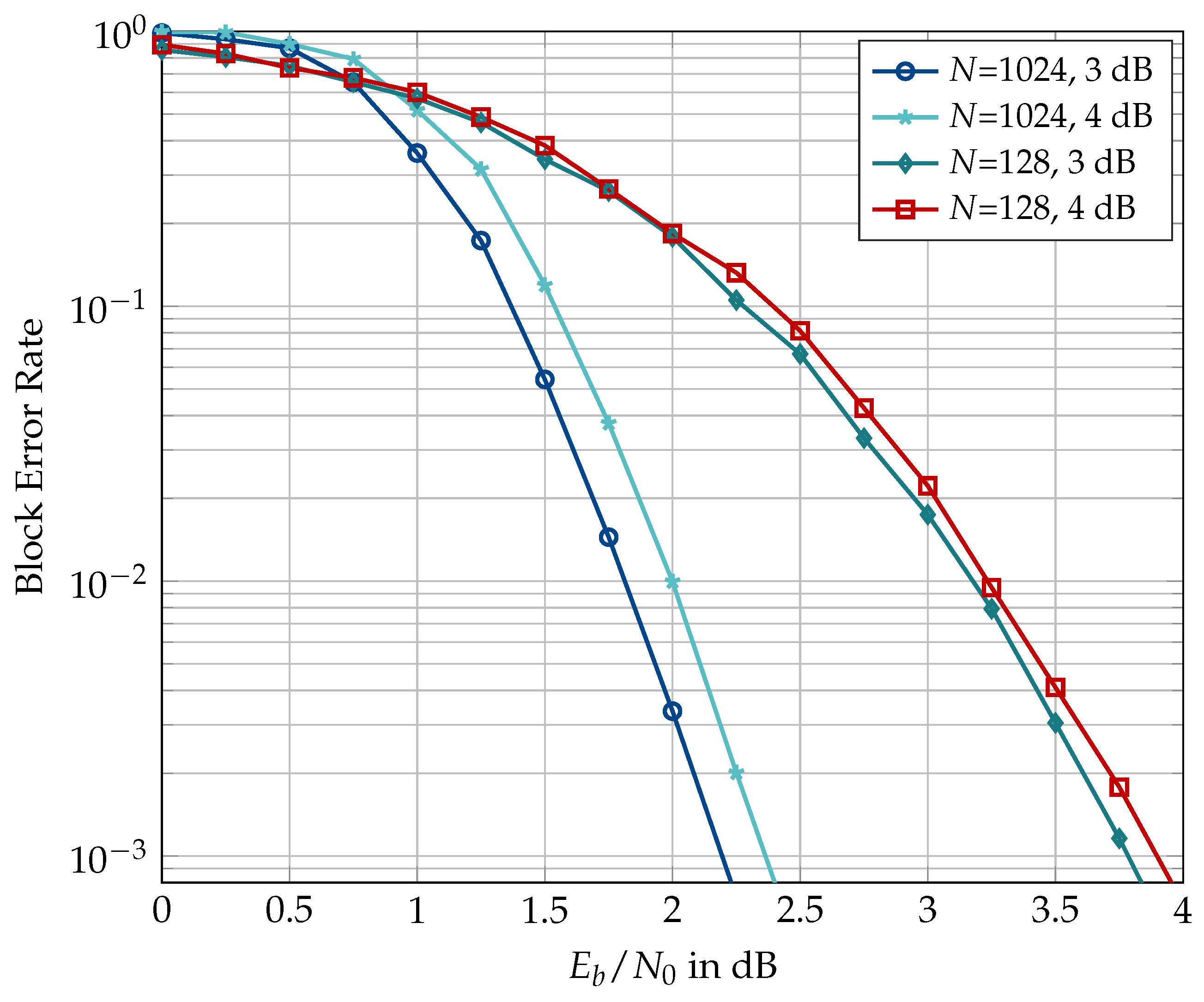
First, Figure 15 and Figure 16 show the block error rate of double-precision floating-point SCL decoder when used with channel quantizers of various bitwidths designed using the information bottleneck method. Figure 15 shows the results for $N=1024$, $N_{crc}=16$, list size $N_L=32$, and quantizer cardinalities $\left|\mathcal{Y}\right|=4,8,16$ or 32. It can be seen that a 5-bit quantizer causes virtually no error rate degradation, whereas the 2-bit quantizer causes $\approx 0.6$ dB degradation at a block error rate of ${10}^{-3}$. Figure 16 shows the results of the same experiment repeated for $N=128$ and $N_L=32$ but without the outer CRC code. The CRC is dropped for the sake of fair comparison with the results of [31] since the author did not use the CRC-aided setting in his experiments. Especially, the results for 2-bit resolution are comparable to those of [31]. Firstly, we see that a channel quantizer with $\left|\mathcal{Y}\right|=16$ shows negligible degradation for the shorter codeword length. Secondly, the 2-bit quantizer causes approximately $0.55$ dB degradation, which is slightly less than the $0.8$ dB degradation reported for the 3-level, i.e., 2-bit, quantizer in Figure 3.1 in [31]. It is, however, pointed out that the code construction methods used in [31] are different than the one used in this document. Based on Figure 15 and Figure 16, $\left|\mathcal{Y}\right|=16$ or 32 seems a good choice to minimize the effect of channel quantization on the decoder performance.

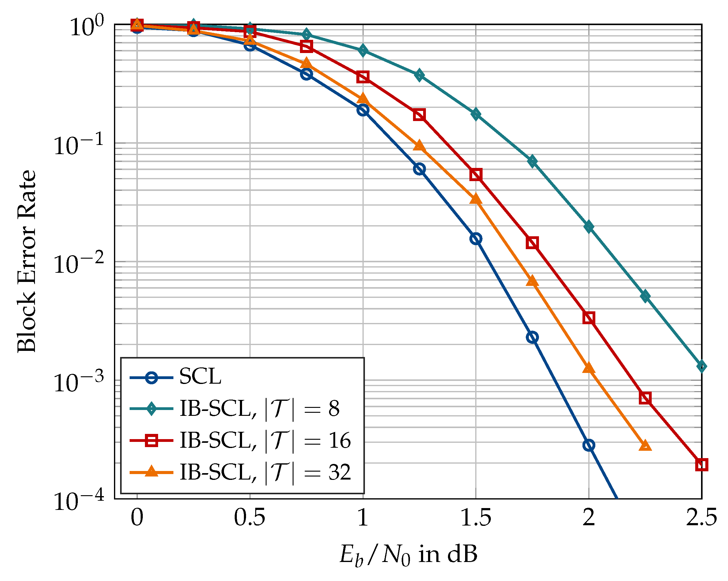
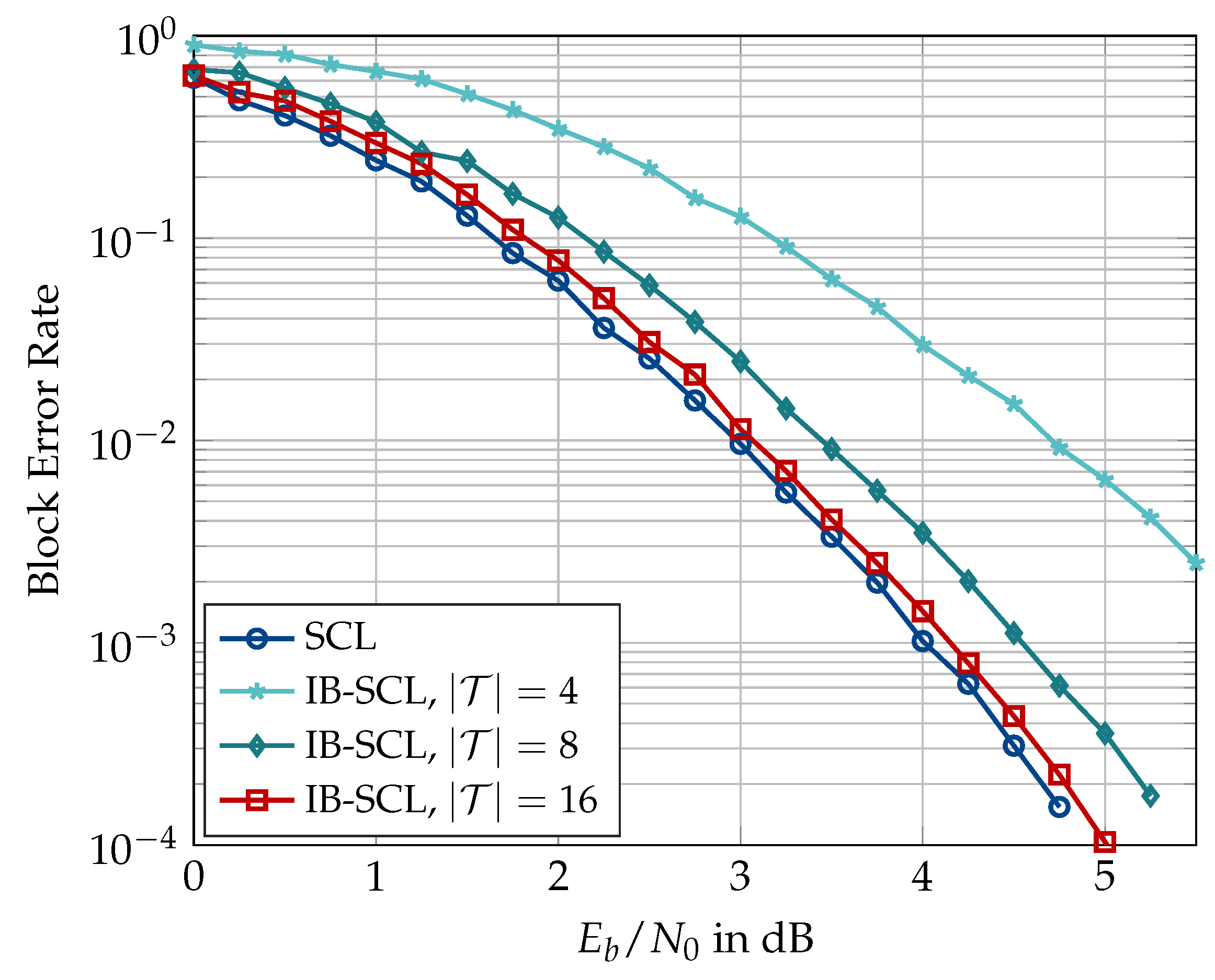
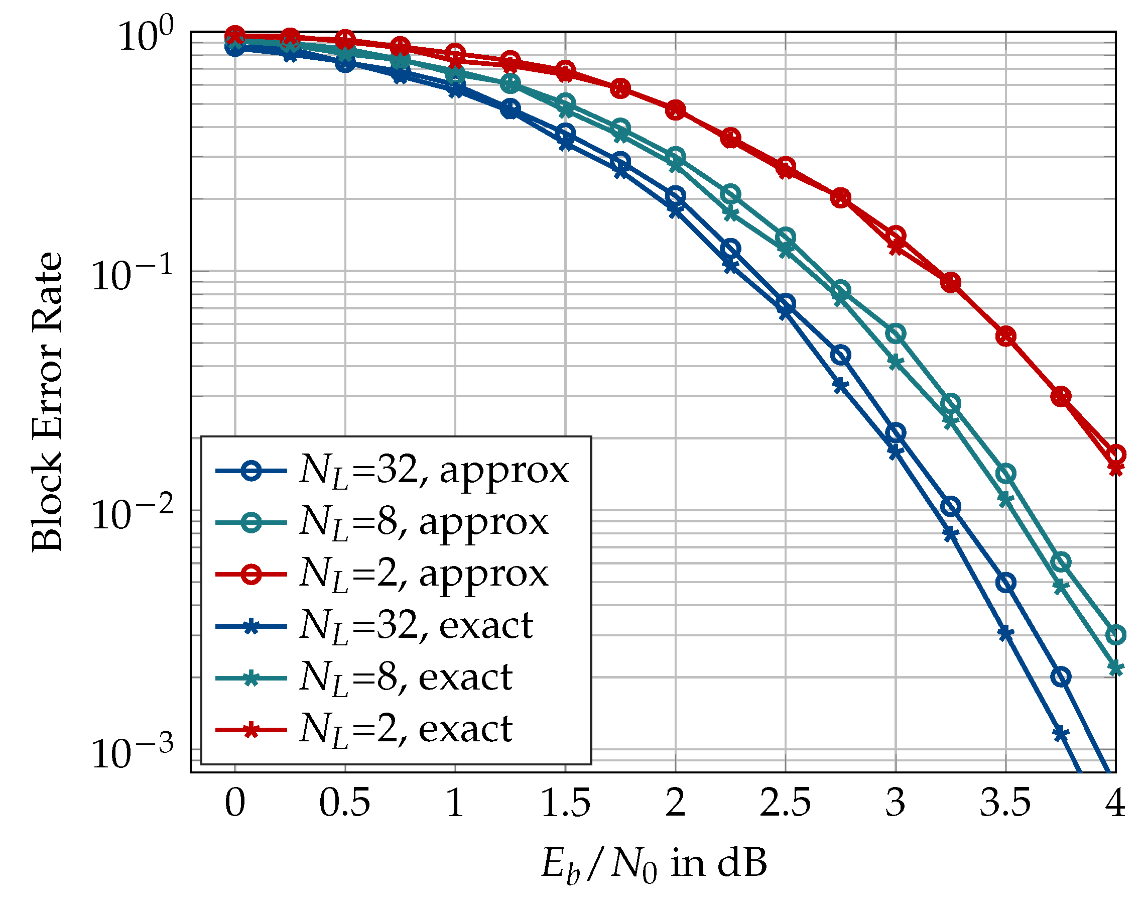
Figure 17, Figure 18, Figure 19, Figure 20, Figure 21 and Figure 22 present simulation results for the information bottleneck decoders without the message alignment. Figure 17 illustrates the trade-off between the space complexity and the performance of the information bottleneck SCL decoders where the quantized decoders for different choices of $\left|\mathcal{T}\right|$ are compared to a conventional SCL decoder for $N=1024$, list size $N_L=32$, and $N_{crc}=16$. As expected, the information bottleneck decoder having the lowest resolution, i.e., $\left|\mathcal{T}\right|=8$ shows the largest degradation of ≈0.65 dB where the channel quantizer contributes $0.25$ dB (as in Figure 15). The performance degradation of the quantized decoding can be reduced to ≈0.33 dB and ≈0.2 dB using decoders constructed for $\left|\mathcal{T}\right|=16$ and $\left|\mathcal{T}\right|=32$, respectively. Figure 18 compares the block error rate of information bottleneck and conventional SCL decoders for $N=128$ and $N_L=32$ without the outer CRC code (cf. Figure 16). It can be seen that the information bottleneck decoders with $\left|\mathcal{T}\right|=16,8$ and 4 show $0.2,0.55$ and $1.9$ dB degradation, respectively, at a block error rate of ${10}^{-3}$. Compared to the information bottleneck decoder with 2-bit resolution, the 3-level quantized decoder of [31] exhibits a degradation of $2.6$ dB for similar decoder parameters (Figure 3.4 in [31]). However, the enhancements proposed in [31] drastically improve the performance of the 3-level quantized SCL decoder and limit the degradation caused by the very coarse quantization to well below $1.5$ dB. For the case of information bottleneck decoders, as presented in this paper, the performance degradation can only be reduced using higher bitwidths, e.g., $\left|\mathcal{T}\right|=16$.

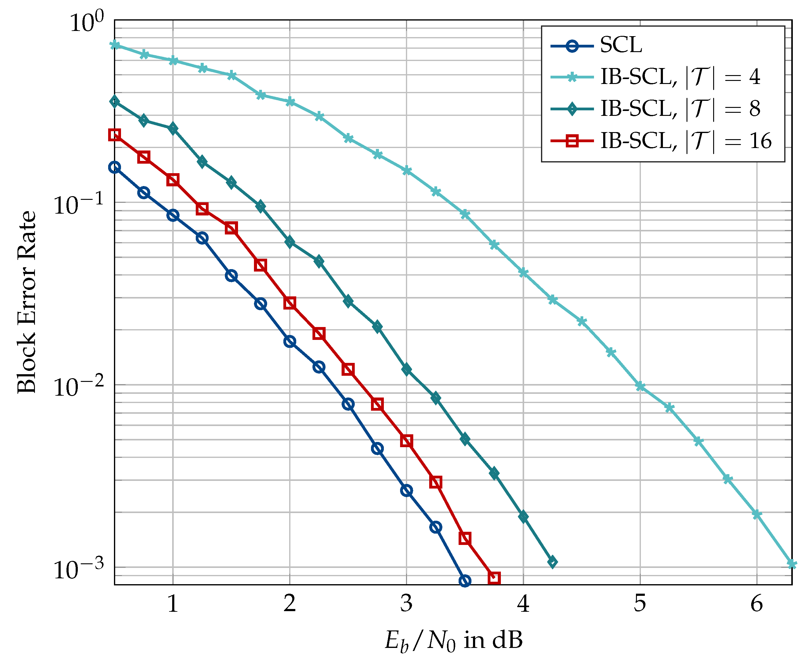
Figure 19 shows the block error rate of an information bottleneck SCL decoder for a low code rate of ≈0.145 with $N=256$, $N_L=32$, no CRC, and design $E_b/N_0=4$ dB. The information bottleneck decoders with $\left|\mathcal{T}\right|=16,8$, and 4 show a degradation of $0.3,0.85$, and $2.9$ dB, respectively, at a block error rate of ${10}^{-3}$. The degradation due to quantization in the information bottleneck decoders is starker (cf. Figure 18) at low code rates in accordance with the theoretical predictions of [28].

In the remainder of this document, the investigations are restricted to information bottleneck decoders having a 4-bit resolution, i.e., $\left|\mathcal{T}\right|=16$. Figure 20 shows the effect of the choice of design $E_b/N_0$ for generating information bottleneck decoders that are used mismatched to the operating $E_b/N_0$ range. The decoders in the figure are used in the CRC-aided setting with $N_{crc}=16$, $N_L=32$, code rate of 0.5, and design $E_b/N_0=3$ or 4 dB. For $N=1024$, the information bottleneck decoder constructed for design $E_b/N_0=4$ dB shows a degradation of $0.15$ dB compared to the one designed for $E_b/N_0=3$ dB at a block error rate of ${10}^{-3}$. This degradation is partly due to the difference in the information sets obtained for the two design $E_b/N_0$ values and partly due to the decoder itself. The evidence for the second part of this statement is provided by the results for $N=128$ in the same figure. Although the information sets generated for design $E_b/N_0=3$ and 4 dB are the same in the case of $N=128$, the decoder designed for $E_b/N_0=4$ dB shows a degradation of $0.1$ dB. Hence, the design $E_b/N_0$ of an information bottleneck decoder needs to be carefully chosen. We have observed that the sensitivity of information bottleneck decoders to design $E_b/N_0$ depends on codeword length N, code rate, and decoder setting, i.e., with or without the outer CRC.

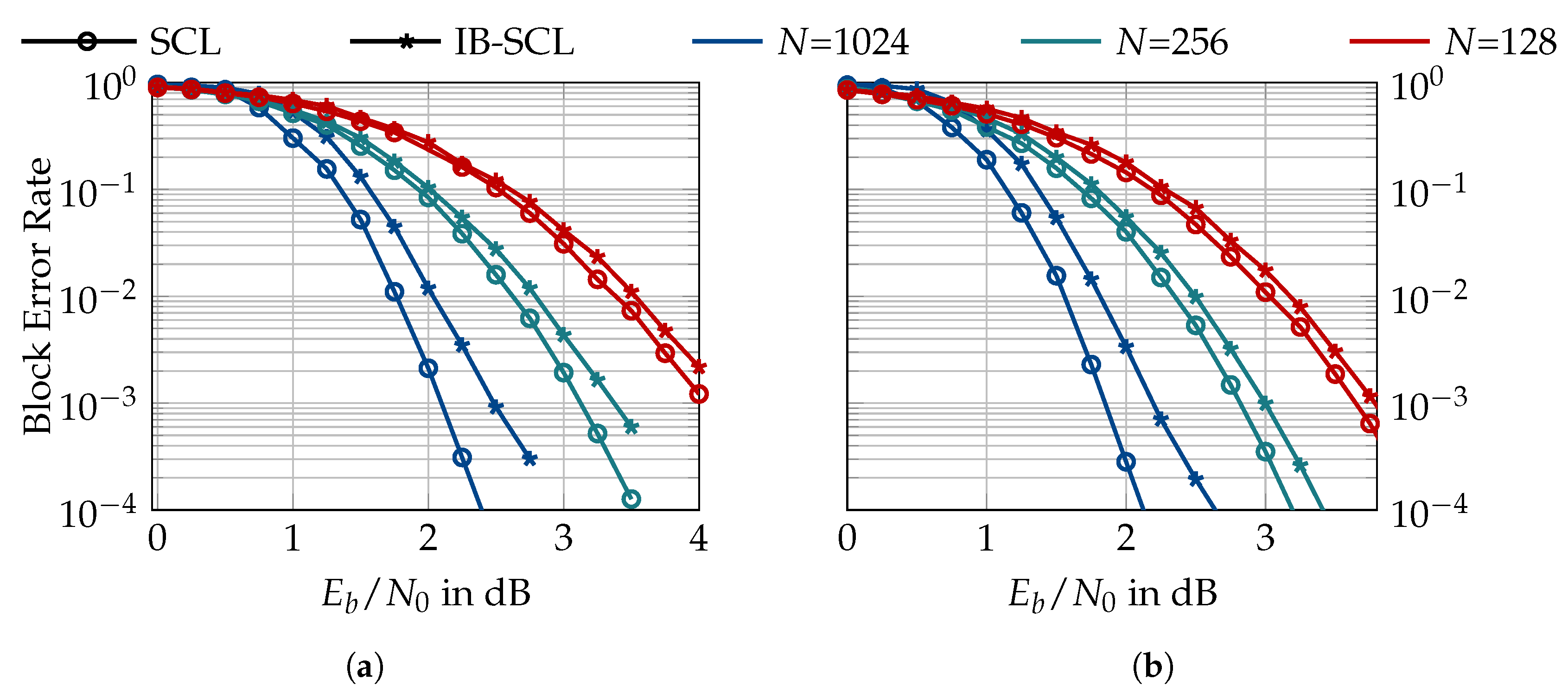
Figure 21a compares the block error rate of the conventional and information bottleneck SCL decoder for a list size of $N_L=8$ and various codeword lengths N. The information bottleneck decoder shows a degradation of approximately $0.16,0.25$, and $0.39$ dB at a block error rate of ${10}^{-3}$ for codeword lengths of $N=128,256$, and 1024, respectively. Figure 21b shows the same comparison for a list size of $N_L=32$, where a gap of $0.13,0.22$, and $0.33$ dB is observed at a block error rate of ${10}^{-3}$ for codeword lengths of $N=128,256$, and 1024, respectively, between the block error rate of the information bottleneck decoder and the conventional scheme. These results suggest that the information bottleneck decoders show a larger performance loss for larger codeword lengths.

The exact computation of the path metric in an SCL decoding scheme according to Equation (9) involves logarithm and exponential functions which are not hardware-friendly. Therefore, the approximation of Equation (10) is preferred for hardware implementation which causes a negligible effect on the error rate of the conventional SCL decoder [27]. Figure 22 shows the effect of using the approximate path metric rule in an information bottleneck decoder for $N=128$ and different list sizes. It can be seen that although the use of the approximate path metric update does not affect the error correction performance of the decoder for a list size $N_L=2$, it does cause a minor performance degradation for larger list sizes. The performance loss caused by the use of the approximate update rule seems to increase with the list size.

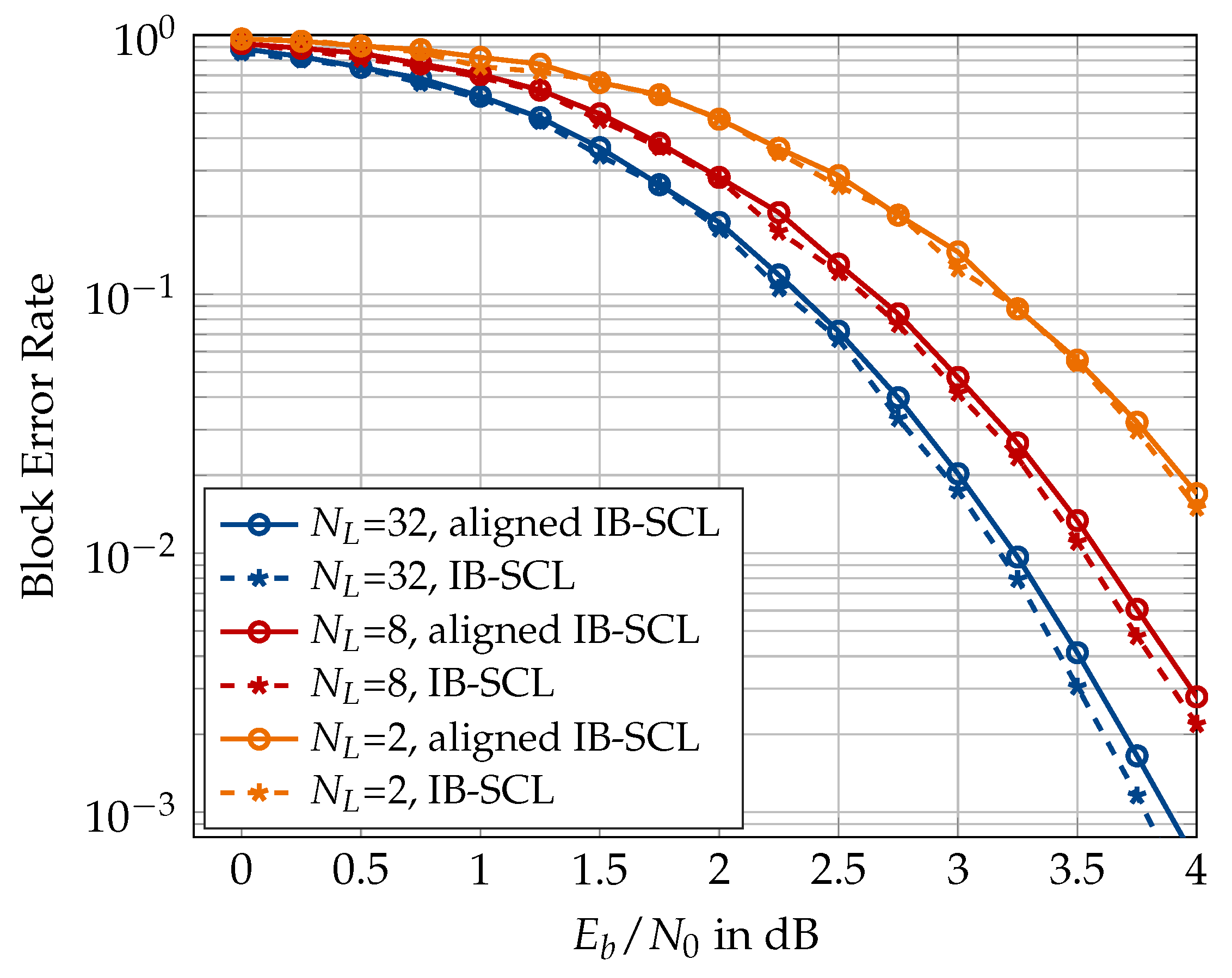
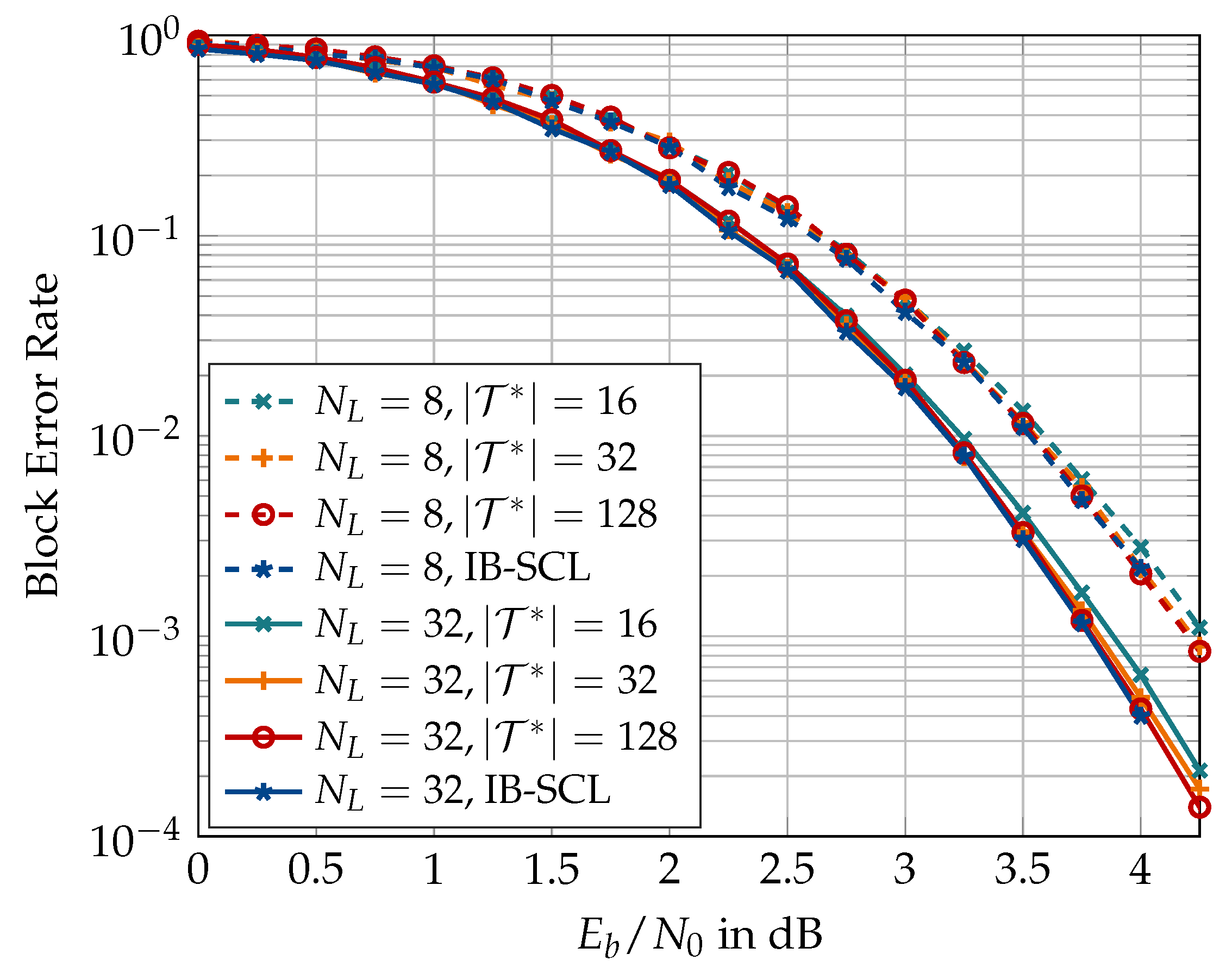
In the following, results on the aligned information bottleneck decoder of Section 5 are presented. First, Figure 23 compares the information bottleneck decoder of Section 4 with its aligned version for $N=128$ and $\left|\mathcal{T}\right|=16$. An alignment cardinality of $|{\mathcal{T}}^{\ast }|=16$ has been used for the translation table alignment in the aligned decoder. It can be seen that the translation table alignment causes a minor degradation of approximately $0.1$ dB for large list size of $N_L=32$, but the degradation vanishes as the list size becomes smaller. Figure 24 shows that the degradation caused by the translation table alignment can effectively be eliminated if a larger alignment cardinality is used, e.g., $|{\mathcal{T}}^{\ast }|=32$ or 128.

The aligned information bottleneck decoder offers several benefits over the information bottleneck decoder of [26]. Firstly, the aligned decoder requires only a single translation table for converting the integer cluster labels into LLR values, regardless of the codeword length N. Recall that the information bottleneck decoder without translation table alignment requires N distinct translation tables. If a $Q_{LLR}=6$ bit resolution is assumed for the LLR values in the translation tables, the information bottleneck decoder without the table alignment of Figure 23 will require $N·\left|\mathcal{T}\right|·Q_{LLR}$ = 12,288 bits to store the N translation tables. On the other hand, the aligned decoder of Figure 23 with $|{\mathcal{T}}^{\ast }|=16$ will require only $|{\mathcal{T}}^{\ast }|·Q_{LLR}=96$ bits for the aligned translation table, thereby reducing the memory required for saving the translation tables by more than 99%. Hence, the aligned decoder is space-efficient in the sense that the space required for storing or implementing the translation table is far less and independent of the codeword length. Secondly, the dynamic range of LLR values stored in the single aligned translation table is significantly smaller than that for N distinct translation tables (cf. Figure 10 and Figure 11). For the polar code of Figure 23, the magnitudes of LLR values stored in the $N=128$ distinct translation tables ranged between 0 and 63. By contrast, the aligned translation table stores LLR magnitudes between 0 and 10, i.e., the LLR values in the aligned translation table require smaller bit resolution. The aligned translation table for $|{\mathcal{T}}^{\ast }|=32$ or 128 (cf. Figure 24) will require 192 or 786 bits of memory, respectively, which is still a considerable reduction. However, recall that translation table alignment with $|{\mathcal{T}}^{\ast }|>|\mathcal{T}|$ increases the bitwidth of the aligned decoding tables at the decision level, which increases their memory requirement. Unfortunately, this increase in the memory requirement of the aligned decoding tables outweighs the savings achieved from the translation table alignment.

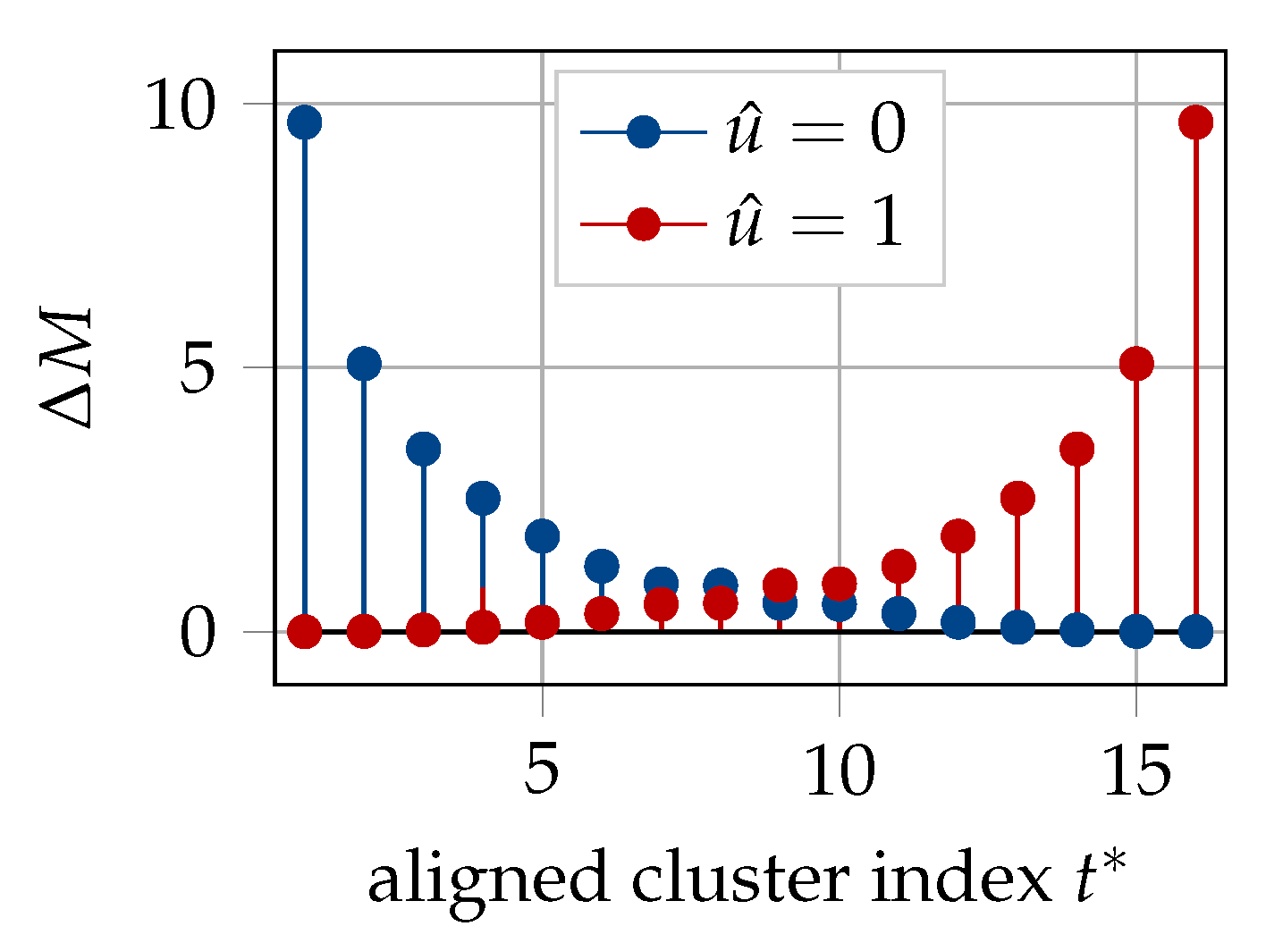
Finally, the fact that only $|{\mathcal{T}}^{\ast }|$ distinct LLR values appear in the aligned information bottleneck SCL decoder can be exploited to circumvent the performance degradation caused be the use of the approximate path metric update rule. Since a single LLR value leads to a single path metric increment in Equation (9) for $\widehat{u}=0$, there exist only $|{\mathcal{T}}^{\ast }|$ path metric increments when a path is extended with $\widehat{u}=0$ at any stage. Owing to the odd symmetry of the translation table (cf. Figure 11), the metric increments for $\widehat{u}=1$ are readily obtained from the increments for $\widehat{u}=0$, as shown in Figure 25. A path metric increment $\Delta M$ in (9) for $t^{\ast }=0,1,2,\dots ,15$, when the decoding path is extended with $\widehat{u}=0$, is equal to $\Delta M$ for $t^{\ast }=15,14,13,\dots ,0$, respectively, if the path is extended with $\widehat{u}=1$. The path metric update values in Figure 25 are computed according to the exact formulation of Equation (9). Therefore, the $|{\mathcal{T}}^{\ast }|$ LLR values in the aligned translation table can be replaced by their respective path increment values, computed offline, for either value of u, and used to translate cluster values $t^{\ast }\in \left\{0,1,\dots ,|{\mathcal{T}}^{\ast }|-1\right\}$ directly into path increments for both the choices of $u\in \left\{0,1\right\}$. As a result, the exact metric update in the aligned information bottleneck decoder is implementation-friendly, i.e., just an addition of real numbers, similar to the approximation of Equation (10).

Perhaps the biggest question on the mind of the reader at this point is how much complexity reduction is achieved using an information bottleneck decoder. Unfortunately, the answer to this question is not straightforward and depends on how the proposed decoder is implemented. The focal point of this paper is to provide a new way to look at quantized polar decoders. Detailed implementation issues are subject to ongoing work.

7. Conclusions

This paper presented the application of the information bottleneck method for construction and coarsely quantized decoding of polar codes. The construction of a polar code requires computing the capacities or error probabilities of its bit channels, whose output alphabet grows exponentially in the codeword length. The information bottleneck framework was used in the discrete density evolution of these virtual bit channels in order to restrict their output alphabet to a small finite size. The quantized bit channels are suitable for capacity or error probability computations. To that end, the famous Tal and Vardy method for constructing polar codes turns out to be equivalent to a particular information bottleneck algorithm. However, they did not fully exploit the benefits offered by the framework. We showed that with the appropriate book-keeping, the hard work done during the discrete density evolution can also be used for decoding. More precisely, the intermediate results of the density evolution, in the form of discrete mappings or lookup tables, are use to replace the LLR computations of conventional successive cancellation list (SCL) decoding. All the operations, except the path metric update, in the information bottleneck SCL decoder are table lookups of unsigned integers. This computational simplicity of the coarsely quantized information bottleneck decoder causes only a small block error rate degradation. The number of lookup tables required in the information bottleneck SCL decoder increases with the codeword length N. We used message alignment to reduce the number of translation tables required to translate the unsigned integer messages into LLR values for the path metric update. The aligned information bottleneck decoder requires only a single translation table regardless of the codeword length and fewer bits to represent the LLR values, which is a reduction in their space complexity. Moreover, the aligned information bottleneck decoders also facilitate a hardware-friendly implementation of the path metric update.

References

- Lewandowsky, J.; Bauch, G. Trellis based node operations for LDPC decoders from the Information Bottleneck method. In Proceedings of the 9th International Conference on Signal Processing and Communication Systems (ICSPCS), Cairns, Australia, 14–16 December 2015; IEEE: Piscataway, NJ, USA, 2015; pp. 1–10. [Google Scholar]
- Lewandowsky, J.; Bauch, G. Information-Optimum LDPC Decoders Based on the Information Bottleneck Method. IEEE Access 2018, 6, 4054–4071. [Google Scholar] [CrossRef]
- Tishby, N.; Pereira, F.C.; Bialek, W. The Information Bottleneck Method. In Proceedings of the 37th Allerton Conference on Communication and Computation, Monticello, IL, USA, 22–24 September 1999. [Google Scholar]
- Slonim, N. The Information Bottleneck: Theory and Applications. Ph.D. Thesis, Hebrew University of Jerusalem, Jerusalem, Israel, 2002. [Google Scholar]
- Kurkoski, B.M.; Yamaguchi, K.; Kobayashi, K. Noise Thresholds for Discrete LDPC Decoding Mappings. In Proceedings of the IEEE GLOBECOM 2008–2008 IEEE Global Telecommunications Conference, New Orleans, LO, USA, 30 November–4 December 2008; pp. 1–5. [Google Scholar]
- Richardson, T.; Urbanke, R. Modern Coding Theory; Cambridge University Press: New York, NY, USA, 2008. [Google Scholar]
- Stark, M.; Lewandowsky, J.; Bauch, G. Information-Bottleneck Decoding of High-Rate Irregular LDPC Codes for Optical Communication Using Message Alignment. Appl. Sci. 2018, 8, 1884. [Google Scholar] [CrossRef]
- Stark, M.; Lewandowsky, J.; Bauch, G. Information-Optimum LDPC Decoders with Message Alignment for Irregular Codes. In Proceedings of the 2018 IEEE Global Communications Conference (GLOBECOM), Abu Dhabi, UAE, 9–13 December 2018; pp. 1–6. [Google Scholar]
- Balatsoukas-Stimming, A.; Meidlinger, M.; Ghanaatian, R.; Matz, G.; Burg, A. A fully-unrolled LDPC decoder based on quantized message passing. In Proceedings of the 2015 IEEE Workshop on Signal Processing Systems SiPS, Hangzhou, China, 14–16 October 2015; pp. 1–6. [Google Scholar] [CrossRef]
- Meidlinger, M.; Balatsoukas-Stimming, A.; Burg, A.; Matz, G. Quantized message passing for LDPC codes. In Proceedings of the 49th Asilomar Conference on Signals, Systems and Computers, Pacific Grove, CA, USA, 8–11 November 2015; pp. 1606–1610. [Google Scholar] [CrossRef]
- Meidlinger, M.; Matz, G. On irregular LDPC codes with quantized message passing decoding. In Proceedings of the 2017 IEEE 18th International Workshop on Signal Processing Advances in Wireless Communications (SPAWC), Sapporo, Japan, 3–6 July 2017; pp. 1–5. [Google Scholar] [CrossRef]
- Ghanaatian, R.; Balatsoukas-Stimming, A.; Müller, T.C.; Meidlinger, M.; Matz, G.; Teman, A.; Burg, A. A 588-Gb/s LDPC Decoder Based on Finite-Alphabet Message Passing. IEEE Trans. Very Large Scale Integr. Syst. 2018, 26, 329–340. [Google Scholar] [CrossRef]
- Arikan, E. Channel Polarization: A Method for Constructing Capacity-Achieving Codes for Symmetric Binary-Input Memoryless Channels. IEEE Trans. Inf. Theory 2009, 55, 3051–3073. [Google Scholar] [CrossRef]
- Hussami, N.; Korada, S.B.; Urbanke, R. Performance of polar codes for channel and source coding. In Proceedings of the 2009 IEEE International Symposium on Information Theory, Seoul, Korea, 28 June–3 July 2009; pp. 1488–1492. [Google Scholar] [CrossRef]
- Bakshi, M.; Jaggi, S.; Effros, M. Concatenated Polar codes. In Proceedings of the 2010 IEEE International Symposium on Information Theory, Austin, TX, USA, 13–18 June 2010; pp. 918–922. [Google Scholar] [CrossRef]
- Tal, I.; Vardy, A. List Decoding of Polar Codes. IEEE Trans. Inf. Theory 2015, 61, 2213–2226. [Google Scholar] [CrossRef]
- Li, B.; Shen, H.; Tse, D. An Adaptive Successive Cancellation List Decoder for Polar Codes with Cyclic Redundancy Check. IEEE Commun. Lett. 2012, 16, 2044–2047. [Google Scholar] [CrossRef]
- Wang, T.; Qu, D.; Jiang, T. Parity-Check-Concatenated Polar Codes. IEEE Commun. Lett. 2016, 20, 2342–2345. [Google Scholar] [CrossRef]
- Nokia. Chairman’s notes of AI 7.1.5 on channel coding and modulation for NR. In Proceedings of the Meeting 87, 3GPP TSG RAN WG1, Reno, NV, USA, 14–19 November 2016. [Google Scholar]
- Arikan, E. A performance comparison of polar codes and Reed-Muller codes. IEEE Commun. Lett. 2008, 12, 447–449. [Google Scholar] [CrossRef]
- ETSI. 5G; NR; Multiplexing and Channel Coding (Release 15); Version 15.6.0; Technical Specification (TS) 38.212, 3rd Generation Partnership Project (3GPP); ETSI: Sophia Antipolis, France, 2019. [Google Scholar]
- Mori, R.; Tanaka, T. Performance of Polar Codes with the Construction using Density Evolution. IEEE Commun. Lett. 2009, 13, 519–521. [Google Scholar] [CrossRef]
- Tal, I.; Vardy, A. How to Construct Polar Codes. IEEE Trans. Inf. Theory 2013, 59, 6562–6582. [Google Scholar] [CrossRef] [Green Version]
- Trifonov, P. Efficient Design and Decoding of Polar Codes. IEEE Trans. Commun. 2012, 60, 3221–3227. [Google Scholar] [CrossRef] [Green Version]
- Stark, M.; Shah, S.A.A.; Bauch, G. Polar code construction using the information bottleneck method. In Proceedings of the 2018 IEEE Wireless Communications and Networking Conference Workshops, Barcelona, Spain, 15–18 April 2018; pp. 7–12. [Google Scholar] [CrossRef]
- Shah, S.A.A.; Stark, M.; Bauch, G. Design of Quantized Decoders for Polar Codes using the Information Bottleneck Method. In Proceedings of the 12th International ITG Conference on Systems, Communications and Coding (SCC 2019), Rostock, Germany, 11–14 February 2019. [Google Scholar]
- Balatsoukas-Stimming, A.; Parizi, M.B.; Burg, A. LLR-based successive cancellation list decoding of polar codes. In Proceedings of the 2014 IEEE International Conference on Acoustics, Speech and Signal Processing (ICASSP), Florence, Italy, 4–9 May 2014; pp. 3903–3907. [Google Scholar] [CrossRef]
- Hassani, S.H.; Urbanke, R. Polar codes: Robustness of the successive cancellation decoder with respect to quantization. In Proceedings of the 2012 IEEE International Symposium on Information Theory Proceedings, Cambridge, MA, USA, 1–6 July 2012; pp. 1962–1966. [Google Scholar] [CrossRef]
- Shi, Z.; Chen, K.; Niu, K. On Optimized Uniform Quantization for SC Decoder of Polar Codes. In Proceedings of the 2014 IEEE 80th Vehicular Technology Conference (VTC2014-Fall), Vancouver, BC, Canada, 14–17 September 2014; pp. 1–5. [Google Scholar] [CrossRef]
- Giard, P.; Sarkis, G.; Balatsoukas-Stimming, A.; Fan, Y.; Tsui, C.; Burg, A.; Thibeault, C.; Gross, W.J. Hardware decoders for polar codes: An overview. In Proceedings of the 2016 IEEE International Symposium on Circuits and Systems (ISCAS), Montreal, QC, Canada, 22–25 May 2016; pp. 149–152. [Google Scholar] [CrossRef]
- Neu, J. Quantized Polar Code Decoders: Analysis and Design. arXiv 2019, arXiv:1902.10395. [Google Scholar]
- Hagenauer, J.; Offer, E.; Papke, L. Iterative decoding of binary block and convolutional codes. IEEE Trans. Inf. Theory 1996, 42, 429–445. [Google Scholar] [CrossRef]
- Lewandowsky, J.; Stark, M.; Bauch, G. Information Bottleneck Graphs for receiver design. In Proceedings of the 2016 IEEE International Symposium on Information Theory (ISIT), Barcelona, Spain, 10–15 July 2016; pp. 2888–2892. [Google Scholar] [CrossRef]
- Stark, M.; Lewandowsky, J. Information Bottleneck Algorithms in Python. Available online: https://goo.gl/QjBTZf (accessed on 25 August 2019).
- Lewandowsky, J.; Stark, M.; Bauch, G. A Discrete Information Bottleneck Receiver with Iterative Decision Feedback Channel Estimation. In Proceedings of the 2018 IEEE 10th International Symposium on Turbo Codes Iterative Information Processing (ISTC), Hong Kong, China, 3–7 December 2018; pp. 1–5. [Google Scholar] [CrossRef]
- Hassanpour, S.; Wuebben, D.; Dekorsy, A. Overview and Investigation of Algorithms for the Information Bottleneck Method. In Proceedings of the 11th International ITG Conference on Systems, Communications and Coding (SCC 2017), Hamburg, Germany, 6–9 February 2017; pp. 1–6. [Google Scholar]
- Lewandowsky, J.; Stark, M.; Bauch, G. Message alignment for discrete LDPC decoders with quadrature amplitude modulation. In Proceedings of the 2017 IEEE International Symposium on Information Theory (ISIT), Aachen, Germany, 25–30 June 2017; pp. 2925–2929. [Google Scholar] [CrossRef]
- Elkelesh, A.; Ebada, M.; Cammerer, S.; ten Brink, S. Decoder-Tailored Polar Code Design Using the Genetic Algorithm. IEEE Trans. Commun. 2019, 67, 4521–4534. [Google Scholar] [CrossRef] [Green Version]
- Wu, D.; Li, Y.; Sun, Y. Construction and Block Error Rate Analysis of Polar Codes Over AWGN Channel Based on Gaussian Approximation. IEEE Commun. Lett. 2014, 18, 1099–1102. [Google Scholar] [CrossRef]
Figure 1.
Factor graph of the building block (dashed rectangle) of a polar code along with the transmission channel.
Figure 2.
Structure of a polar code with . The graph is partitioned into levels. The node labels, indicate the vertical stage, , and horizontal level, . For all i, , i.e., the channel output at level , while , i.e., the encoder input bits at level .
Figure 3.
(a) Information bottleneck setup, where is the relevant information, is the original mutual information, and is the compression information. The goal is to determine the mapping which maximizes and minimizes . (b) Information bottleneck graph for the elementary setup of (a). The realizations of Y are mapped onto those of T such that their relevance to X is preserved, i.e., , and .
Figure 4.
Transition probability of AWGN channel where continuous channel output is clustered into bins or clusters for . (a) Randomly initialized symmetric cluster boundaries. (b) Cluster boundaries optimized such that is maximum for .
Figure 5.
Information bottleneck graph for (a) the bit channel of which maps outputs onto clusters, labeled , treating as the relevant variable. (b) The bit channel of which maps the outputs onto clusters, labeled , treating as the relevant variable.
Figure 6.
Information bottleneck graph of a polar code with length . The outputs of the bit channel experienced by each node are clustered into a compressed random variable , where indicates the stage, while represents the level in the code structure.
Figure 7.
Plot of the cumulative product indicating the amount of mutual information preserved over the levels of a half-rate polar code with depending on the number of clusters .
Figure 8.
(a) Clustering that maps the outputs of the bit channel of to clusters, written as a lookup table. (b) Translation table of obtained from the conditional distribution as in Equation (21).
Figure 9.
Translation tables of an information bottleneck decoder with for different bit channels of a half-rate polar code with , design dB. is a frozen bit while , and are information bits.
Figure 10.
Information bottleneck graph for the alignment of the translation tables of a polar code. The decision level cluster indices are clustered into aligned indices such that the relevant information is maximized.
Figure 11.
Translation table for aligned decoding tables at the decision level with for the polar code with , rate = 0.5 and design dB.
Figure 12.
Frozen charts for half-rate polar code with and design dB, constructed using (a) Tal and Vardy’s method with , (b) Tal and Vardy’s method with , (c) information bottleneck method with , (d) information bottleneck method with , and (e) Gaussian approximation.
Figure 13.
Figure 14.
Block error rate of polar codes constructed using Gaussian approximation, Tal and Vardy’s method, and the information bottleneck method using a conventional successive cancellation (SC) and successive cancellation list (SCL) decoder with , 16-bit cyclic redundancy check (CRC), , rate 0.5, and design dB.
Figure 15.
Block error rate of double-precision floating-point SCL decoder with channel quantizers of different resolutions designed using the information bottleneck method. , , , code rate 0.5, and design dB.
Figure 16.
Block error rate of double-precision floating-point SCL decoder with channel quantizers of different resolutions designed using the information bottleneck method. without the outer CRC code, , code rate 0.5, and design dB.
Figure 17.
Block error rate comparison between conventional decoder (SCL) and information bottleneck decoders (IB-SCL) constructed for or 32. , , 16-bit CRC, code rate 0.5, and design dB.
Figure 18.
Block error rate comparison between conventional decoder (SCL) and information bottleneck decoders (IB-SCL) constructed for or 16. , , no CRC, code rate 0.5, and design dB.
Figure 19.
Block error rate comparison between conventional decoder (SCL) and information bottleneck decoders (IB-SCL) constructed for or 16. , , no CRC, code rate , and design dB.
Figure 20.
Effect of design in the mismatched use of the information bottleneck decoders. or 1024, , , , , and code rate 0.5.
Figure 21.
Block error rate of conventional (SCL) and a 4-bit information bottleneck (IB-SCL) decoders for and 128, rate 0.5, 16-bit CRC design dB. (a) , (b) .
Figure 22.
Effect of using the approximation path metric update rule of Equation (10) on the block error rate of a 4-bit information bottleneck decoder with or 32, 16-bit CRC, , rate 0.5, and design dB.
Figure 23.
Block error rate of a 4-bit aligned information bottleneck SCL decoder with alignment cardinality , 16-bit CRC, , or 32.
Figure 24.
Effect of alignment cardinality on the block error rate of a 4-bit aligned information bottleneck SCL decoder with or 32, 16-bit CRC for , rate 0.5, and design dB.
Figure 25.
Path metric increments computed for the aligned translation table of Figure 11 according to Equation (9). for the polar code with , rate = 0.5, and design dB.
© 2019 by the authors. Licensee MDPI, Basel, Switzerland. This article is an open access article distributed under the terms and conditions of the Creative Commons Attribution (CC BY) license (http://creativecommons.org/licenses/by/4.0/).
Share and Cite
MDPI and ACS Style
Shah, S.A.A.; Stark, M.; Bauch, G. Coarsely Quantized Decoding and Construction of Polar Codes Using the Information Bottleneck Method. Algorithms 2019, 12, 192. https://doi.org/10.3390/a12090192
AMA Style
Shah SAA, Stark M, Bauch G. Coarsely Quantized Decoding and Construction of Polar Codes Using the Information Bottleneck Method. Algorithms. 2019; 12(9):192. https://doi.org/10.3390/a12090192
Chicago/Turabian StyleShah, Syed Aizaz Ali, Maximilian Stark, and Gerhard Bauch. 2019. "Coarsely Quantized Decoding and Construction of Polar Codes Using the Information Bottleneck Method" Algorithms 12, no. 9: 192. https://doi.org/10.3390/a12090192
Note that from the first issue of 2016, this journal uses article numbers instead of page numbers. See further details here.