Learning Output Reference Model Tracking for Higher-Order Nonlinear Systems with Unknown Dynamics †


Department of Automation and Applied Informatics, Politehnica University of Timisoara, 2 Bd. V. Parvan, 300223 Timisoara, Romania
*
Author to whom correspondence should be addressed.
†
This paper is an extended version of our paper published in the 27th Mediterranean Conference on Control and Automation (MED 2019).
Algorithms 2019, 12(6), 121; https://doi.org/10.3390/a12060121
Submission received: 1 May 2019
/
Revised: 7 June 2019
/
Accepted: 9 June 2019
/
Published: 12 June 2019
(This article belongs to the Special Issue Algorithms for PID Controller 2019)
Abstract
:This work suggests a solution for the output reference model (ORM) tracking control problem, based on approximate dynamic programming. General nonlinear systems are included in a control system (CS) and subjected to state feedback. By linear ORM selection, indirect CS feedback linearization is obtained, leading to favorable linear behavior of the CS. The Value Iteration (VI) algorithm ensures model-free nonlinear state feedback controller learning, without relying on the process dynamics. From linear to nonlinear parameterizations, a reliable approximate VI implementation in continuous state-action spaces depends on several key parameters such as problem dimension, exploration of the state-action space, the state-transitions dataset size, and a suitable selection of the function approximators. Herein, we find that, given a transition sample dataset and a general linear parameterization of the Q-function, the ORM tracking performance obtained with an approximate VI scheme can reach the performance level of a more general implementation using neural networks (NNs). Although the NN-based implementation takes more time to learn due to its higher complexity (more parameters), it is less sensitive to exploration settings, number of transition samples, and to the selected hyper-parameters, hence it is recommending as the de facto practical implementation. Contributions of this work include the following: VI convergence is guaranteed under general function approximators; a case study for a low-order linear system in order to generalize the more complex ORM tracking validation on a real-world nonlinear multivariable aerodynamic process; comparisons with an offline deep deterministic policy gradient solution; implementation details and further discussions on the obtained results.
1. Introduction
The output reference model (ORM) tracking problem is of significant interest in practice, especially for nonlinear systems control, since by selection of a linear ORM, feedback linearization is enforced on the controlled process. Then, the closed-loop control system can act linearly in a wide range and not only in the vicinity of an operating point. Subsequently, linearized control systems are then subjected to higher level learning schemes such as the Iterative Learning Control ones, with practical implications such as primitive-based learning [1] that can extrapolate optimal behavior to previously unseen tracking scenarios.
On another side, selection of a suitable ORM is not straightforward because of several reasons. The ORM has to be matched with the process bandwidth and with several process nonlinearities such as, e.g., input and output saturations. From classical control theory, dead-time and non-minimum-phase characters of the process cannot be compensated for and must be reflected in the ORM. Apart from this information that can be measured or inferred from working experience with the process, avoiding knowledge of the process’ state transition function (process dynamics)—the most time consuming to identify and the most uncertain part of the process—in designing high performance control is very attractive in practice.
Reinforcement Learning (RL) has developed both from the artificial intelligence [2], and from classical control [3,4,5,6,7], where it is better known as Adaptive (Approximate, Neuro) Dynamic Programming (ADP). Certain ADP variants can ensure ORM tracking control without knowing the state-space (transition function) dynamics of the controlled process, which is of high importance in the practice of model-free (herein accepted as unknown dynamics) and data-driven control schemes that are able to compensate for poor modeling and process model uncertainty. Thus, ADP relies only on data collected from the process called state transitions. While plenty of mature ADP schemes already exist in the literature, tuning such schemes for a particular problem requires significant experience. Firstly, it must be specified whether ADP deals with continuous (infinite) or discrete (finite) state-action spaces. Then, the intended implementation will decide upon online/offline and/or adaptive/batch processing, the suitable selection of the approximator used for the extended cost function (called the Q-function) and/or for the controller. Afterwards, linear or nonlinear parameterizations are sought. Exploration of the state-action spaces is critical, as well as the hyperparameters of the overall learning scheme such as the number of transition samples, trading off exploration with exploitation, etc. Although successful stories on RL and ADP applied to large state-action spaces are reported mainly with artificial intelligence [8], in control theory, most approaches use low-order processes as representative case studies and mainly in linear quadratic regulator (LQR)-like settings (regulating states to zero). While, in an ADP, the reference input tracking control problem has been tackled before for linear time-invariant (LTI) processes by the name of Linear Quadratic Tracking (LQT) [9,10], the ORM tracking for nonlinear processes was rarely addressed [11,12].
The iterative model-free approximate Value Iteration (IMF-AVI) proposed in this work belongs to the family of batch-fitted Q-learning schemes [13,14] known as action-dependent heuristic dynamic programming (ADHDP) that are popular and representative ADP approaches, owing to their simplicity and model-free character. These schemes have been implemented in many variants: online vs. offline, adaptive or batch, for discrete/continuous states and actions, with/without function approximators, such as Neural Networks (NNs) [12,15,16,17,18,19,20,21,22,23].
Concerning the exploration issue in ADP for control, a suitable exploration that covers as well as possible the state-action space is not trivially ensured. Randomly generated control input signals will almost surely fail to guide the exploration in the entire state-action space, at least not in a reasonable amount of time. Then, a priori designed feedback controllers can be used under a variable reference input serving to guide the exploration [24]. The existence of an initial feedback stabilizing controller, not necessarily of a high performance one, can accelerate the transition samples dataset collection under exploration. This allows for offline IMF-AVI based on large datasets, leading to improved convergence speed for high-dimensional processes. However, such input–output (IO) or input-state feedback controllers were traditionally not to be designed without using a process model, until the advent of data-driven model-free controller design techniques that have appeared from the field of control theory: Virtual Reference Feedback Tuning (VRFT) [25], Iterative Feedback Tuning [26], Model Free Iterative Learning Control [27,28,29], Model Free (Adaptive) Control [30,31], with representative applications [32,33,34]. This work shows a successful example of a model-free output feedback controller used to collect input-to-state transition samples from the process for learning state-feedback ADP-based ORM tracking control. Therefore it fits with the recent data-driven control [35,36,37,38,39,40,41,42,43] and reinforcement learning [12,44,45] applications.
The case study deals with the challenging ORM tracking control for a nonlinear real-world two-inputs–two-outputs aerodynamic system (TITOAS) having six natural states that are extended with four additional ones according to the proposed theory. The process uses aerodynamic thrust to create vertical (pitch) and horizontal (azimuth) motion. It is shown that IMF-AVI can be used to attain ORM tracking of first order lag type, despite the high order of the multivariable process, and despite the pitch motion being naturally oscillatory and the azimuth motion practically behaving close to an integrator. The state transitions dataset is collected under the guidance of an input–output (IO) feedback controller designed using model-free VRFT (© 2019 IEEE [12]).
As a main contribution, the paper is focused on a detailed comparison of the advantages and disadvantages of using linear and nonlinear parameterizations for the IMF-AVI scheme, while covering complete implementation details. To the best of authors’ knowledge, the ORM tracking context with linear parameterizations was not studied before for high-order real-world processes. Moreover, theoretical analysis shows convergence of the IMF-AVI while accounting for approximation errors and explains for the robust learning convergence of the NN-based IMF-AVI. The results indicate that the nonlinearly parameterized NN-based IMF-AVI implementation should be de facto in practice since, although more time-consuming, it automatically manages the basis function selection, it is more robust to dataset size and exploration settings, and generally more well-suited for nonlinear processes with unknown dynamics. The main updates with respect to our paper [12] include: detailed IMF-AVI convergence proofs under general function approximators; a case study for a low order linear system in order to generalize to the more complex ORM tracking validation on the TITOAS process; comparisons with an offline Deep Deterministic Policy Gradient solution; more implementation details and further discussions on the obtained results.
2. Output Model Reference Control for Unknown Dynamics Nonlinear Processes
2.1. The Process
A discrete-time nonlinear unknown open-loop stable state-space deterministic strictly causal process is defined as [12,46]
where k indexes the discrete time, is the n-dimensional state vector, is the control input signal, is the measurable controlled output, is an unknown nonlinear system function continuously differentiable within its domain, is an unknown nonlinear continuously differentiable output function. Initial conditions are not accounted for at this point. Assume known domains are compact convex. Equation (1) is a general un-restrictive form for most controlled processes. The following assumptions common to the data-driven formulation are [12,46]:
Assumption 1 (A1).
(1) is fully state controllable with measurable states.
Assumption 2 (A2).
(1) is input-to-state stable on known domain .
Assumption 3 (A3).
(1) is minimum-phase (MP).
A1 and A2 are widely used in data-driven control, cannot be checked analytically for the unknown model (1) but can be inferred from historical and working knowledge with the process. Should such information not be available, the user can attempt process control under restraining safety operating conditions, that are usually dealt with at supervisory level control. Input to state stability (A2) is necessary if open-loop input-state samples collection is intended to be used for state space control design. Assumption A2 can be relaxed if a stabilizing state-space controller is already available and used just for the purpose of input-state data collection. A3 is the least restrictive assumption and it is used in the context of the VRFT design of a feedback controller based on input–output process data. Although solutions exist to deal with nonminimum-phase systems processes, the MP assumption simplifies the VRFT design and the output reference model selection (to be introduced in the following section).
Comment 1.
[46] Model (1) accounts for a wide range of processes including fixed time-delay ones. For positive integer nonzero delay d on the control input , additional states can extend the initial process model (1) as and arrive at a state-space model without delays, in which the additional states are measurable as past input samples. A delay in the original states in (1), i.e., , are similarly treated.
2.2. Output Reference Model Control Problem Definition
Let the discrete-time known open-loop stable minimum-phase (MP) state-space deterministic strictly causal ORM be [12,46]
where is the ORM state, is the reference input signal, is the ORM output, , are known nonlinear mappings. Initial conditions are zero unless otherwise stated. Notice that are size p for square feedback control systems (CSs). If the ORM (2) is LTI, it is always possible to express the ORM as an IO LTI transfer function (t.f.) ensuring , where is commonly an asymptotically stable unit-gain rational t.f. and is the reference input that drives both the feedback CS and the ORM. We introduce an extended process comprising of the process (1) coupled with the ORM (2). For this, we consider the reference input as a set of measurable exogenous signals (possibly interpreted as a disturbance) that evolve according to , with known nonlinear , where is measurable. Herein, is a generative model for the reference input (© 2019 IEEE [12]).
The class of LTI generative models has been studied before in [9] but it is a rather restrictive one. For example, reference inputs signals modeled as a sequence of steps of constant amplitude cannot be modeled by LTI generative models. A step reference input signal with constant amplitude over time can be modeled as with some initial condition . On the other hand, a sinusoidal scalar reference input signal can be modeled only through a second order state-space model. To see this, let the Laplace transform of ( is the unit step function) be with the complex Laplace variable s. If is considered a t.f. driven by the unit step function with Laplace transform , then the LTI discrete-time state-space associated with acting as a generative model for is of the form
with known , and is the discrete-time unit step function. The combination of driven by the Dirac impulse with could also have been considered as a generative model. Based on the state-space model above, modeling p sinusoidal reference inputs requires states. Generally speaking, the generative model of the reference input must obey the Markov property.
Consider next that the extended state-space model that consists of (1), (2), and the state-space generative model of the reference input signal is, in the most general form [12,46]:
where is called the extended state vector. Note that the extended state-space fulfils the Markov property. The ORM tracking control problem is formulated in an optimal control framework. Let the infinite horizon cost function (c.f.) to be minimized starting with be [6,12,46]
In (5), the discount factor sets the controller’s horizon, is usually used in practice to guarantee learning convergence to optimal control. is the Euclidean norm of the column vector . is the stage cost where measurable depends via unknown in (1) on and penalizes the deviation of from the ORM’s output . In ORM tracking, the stage cost does not penalize the control effort with some positive definite function since the ORM tracking instills an inertia on the CS that indirectly acts as a regularizer on the control effort. Secondly, if the reference inputs do not set to zero, the ORM’s outputs also do not. For most processes, the corresponding constant steady-state control will be non-zero, hence making infinite when [12,46].
Herein, parameterizes a nonlinear state-feedback admissible controller [6] defined as , which used in (4) shows that all CS’s trajectories depend on . Any stabilizing controller sequence (or controller) rendering a finite c.f. is called admissible. A finite holds if is a square-summable sequence, ensured by an asymptotically stabilizing controller if or by a stabilizing controller if . in (5) is the value function of using the controller . Let the optimal controller that minimizes (5) be [12,46]
Tracking a nonlinear ORM can also be used, however, tracking a linear one renders highly desirable indirect feedback linearization of the CS, where a linear CS’s behavior generalizes well in wide operating ranges [1]. Then the ORM tracking control problem of this work should make when drives both the CS and the ORM.
Under classical control rules, following Comment 1, the process time delay and non-minimum-phase (NMP) character should be accounted for in . However, the NMP zeroes make non-invertible in addition to requiring their identification, thus placing a burden on the subsequent VRFT IO control design [47]. This motivates the MP assumption on the process.
Depending on the learning context, the user may select a piece-wise constant generative model for the reference input signal such as , or a ramp-like model, a sine-like model, etc. In all cases, the states of the generative model are known, measurable and need to be introduced in the extended state vector, to fulfill the Markov property of the extended state-space model. In many practical applications, for the ORM tracking problem, the CS’s outputs are required to track the ORM’s outputs when both the ORM and the CS are driven by the piece-wise constant reference input signal expressed by a generative model of the form . This generative model will be used subsequently in this paper for learning ORM tracking controllers. Obviously, the learnt solution will depend on the proposed reference input generative model, while changing this model requires re-learning.
3. Solution to the ORM Tracking Problem
For unknown extended process dynamics (4), minimization of (5) can be tackled using an iterative model-free approximate Value Iteration (IMF-AVI). A c.f. that extends called the Q-function (or action-value function) is first defined for each state-action pair. Let the Q-function of acting as in state and then following the control (policy) be [12,46]
The optimal Q-function corresponding to the optimal controller obeys Bellman’s optimality equation [12,46]
where the optimal controller and Q-functions are [12,46]
Then, for it follows that . Implying that finding is equivalent to finding the optimal c.f. .
The optimal Q-function and optimal controller can be found using either Policy Iteration (PoIt) or Value Iteration (VI) strategies. For continuous state-action spaces, IMF-AVI is one possible solution, using different linear and/or nonlinear parameterizations for the Q-function and/or for the controller. NNs are most widely used as nonlinearly parameterized function approximators. As it is well-known, VI alternates two steps: the Q-function estimate update step and the controller improvement step. Several Q-function parameterizations allow for explicit analytic calculation of the improved controller as the following optimization problem (© 2019 IEEE [12])
by directly minimizing w.r.t. , where the parameterization has been moved from the controller into the Q-function. (10) is the controller improvement step specific to both the PoIt and VI algorithms. In these special cases, it is possible to eliminate the controller approximator and use only one for the Q-function Q. Then, given a dataset D of transition samples, the IMF-AVI amounts to solving the following optimization problem (OP) at every iteration j (© 2019 IEEE [12])
which is a Bellman residual minimization problem where the (usually separate) controller improvement step is now embedded inside the OP (11). More explicitly, for a linear parameterization using a set of basis functions of the form , the least squares solution to (11) is equivalent to solving the following over-determined linear system of equations w.r.t. in the least-squares sense (© 2019 IEEE [12]):
Concluding, starting with an initial parameterization , the IMF-AVI approach with linearly parameterized Q-function that allows explicit controller improvement calculation as in (10), embeds both VI steps into solving (12). Linearly parameterized IMF-AVI (LP-IMF-AVI) will be validated in the case study and compared to nonlinearly parameterized IMF-AVI (NP-IMF-AVI). Convergence of the generally formulated IMF-AVI is next analysed under approximation errors (© 2019 IEEE [12]).
IMF-AVI Convergence Analysis with Approximation Errors for ORM Tracking
The proposed iterative model-free VI-based Q-learning Algorithm 1 consists of the next steps (© 2019 IEEE [12]).
| Algorithm 1 VI-based Q-learning. |
| S1: Initialize controller and the Q-function value to , initialize iteration index |
| S2: Use one step backup equation for the Q-function as in (13) |
| S3: Improve the controller using the Equation (14) |
| S4: Set and repeat steps S2, S3, until convergence |
To be detailed as follows:
S1. Select an initial (not necessarily admissible) controller and an initialization value of the Q-function. Initialize iteration .
S2. Use one step backup equation for the Q-function
S3. Improve the controller using the equation
S4. Set and repeat steps S2, S3, until convergence.
Lemma 1.
(© 2019 IEEE [12]) For an arbitrary sequence of controllers define the VI-update for extended c.f. as [48]
If , then .
Proof.
It is valid that
Meaning that . Assume by induction that . Then
which completes the proof. Here, it was used that is the optimal controller for per (14), then, for any other controller (in particular it can also be ) it follows that
□
Lemma 2.
(© 2019 IEEE [12]) For the sequence {} from (13), under controllability assumption A1, it is valid that:
- (1)
- with an upper bound.
- (2)
- If there exists a solution to (8), then .
Proof.
For any fixed admissible controller , is the Bellman equation. Update (13) renders
Replacing from the last inequality towards the first it follows that
then, setting proves the first part of Lemma 2.
Among all admissible controllers, the optimal one renders the Q-function with the lowest value therefore . If is the optimal controller, it follows that . Then the second part of Lemma 2 follows as . □
Theorem 1.
(© 2019 IEEE [12]) For the extended process (4) under A1, A2, with c.f. (5), with the sequences {} and {} generated by the Q-learning Algorithm 1, it is true that:
- (1)
- {} is a non-decreasing sequence for which holds, and
- (2)
- (2) and .
Proof.
Let and assume the update
By induction it is shown that since
Assume next that and show that
The expression above leads to . Since by Lemma 1 one has that it follows that , proving first part of Theorem 1.
Any non-decreasing upper bounded sequence must have a limit, thus and with an admissible controller. For any admissible controller that is non-optimal if follows from (20) that . Still, part 2 of Lemma 2 states that implying . Then from it must hold true that and which proves the second part of Theorem 1. □
Comment 2.
(© 2019 IEEE [12]) (13) is practically solved in the sense of the OP (11) (either as a linear or nonlinear regression) using a batch (dataset) of transition samples collected from the process using any controller, that is in off-policy mode. While the controller improvement step (14) can be solved either as a regression or explicitly analytically when the expression of allows it. Moreover, (13) and (14) can be solved batch-wise in either online or offline mode. When the batch of transition samples is updated with one sample at a time, the VI-scheme becomes adaptive.
Comment 3.
(© 2019 IEEE [12]) Theorem 1 proves the VI-based learning convergence of the sequence of Q-functions assuming that the true Q-function parameterization is used. In practice, this is rarely possible, such as, e.g., in the case of LTI systems. For general nonlinear processes of type (1), different function approximators are employed for the Q-function, most commonly using NNs. Then the convergence of the VI Q-learning scheme is to a suboptimal controller and to a suboptimal Q-function, owing to the approximation errors. A generic convergence proof of the learning scheme under approximation errors is next shown, accounting for general Q-function parameterizations [49].
Let the IMF-AVI Algorithm 2 consist of the steps (© 2019 IEEE [12]).
| Algorithm 2 IMF-AVI. |
| S1: Initialize controller and Q-function value . Initialize iteration |
| S2: Update the approximate Q-function using Equation (24) |
| S3: Improve the approximate controller using Equation (25) |
| S4: Set and repeat steps S2, S3, until convergence |
To be detailed as follows:
S1. Select an initial (not necessarily admissible) controller and an initialization value of the Q-function. Initialize iteration .
S2. Use the update equation for the approximate Q-function
S3. Improve the approximate controller using
S4. Set and repeat steps S2, S3, until convergence.
Comment 4.
(© 2019 IEEE [12]) In Algorithm 2, the sequences and are approximations of the true sequences and . Since the true Q-function and controller parameterizations are not generally known, (24) must be solved in the sense of the OP (11) with respect to the unknown , in order to minimize the residuals at each iteration. If the true parameterizations of the Q-function and of the controller were known, then and the IMF-AVI updates (24), (25) coincide with (13), (14), respectively. Next, let the following assumption hold.
A4. ([12]) There exist two positive scalar constants such that , ensuring
Comment 5.
(© 2019 IEEE [12]) Inequalities from (26) account for nonzero positive or negative residuals , i.e., for the approximation errors in the Q-function, since can over- or under-estimate in (24). can span large intervals ( close to 0 and very large). The hope is that, if are close to 1—meaning low approximation errors—then the entire IMF-AVI process preserves . In practice, this amounts to using high performance approximators. For example, with NNs, adding more layers and more neurons, enhances the approximation capability and theoretically reduces the residuals in (24).
Theorem 2.
Let the sequences and evolve as in (24), (25), the sequences and evolve as in (13), (14). Initialize and let A3 hold. Then
Proof.
(© 2019 IEEE [12]) First, the development proceeds by induction for the left inequality. For it is clear that . For , (13) produces and left-hand side of (26) reads . Then . Next assume that
holds at iteration j. Based on (28) used in (26), it is valid that
Notice from (29) that
From (29), (30) it follows that proving the left side of (27) by induction. The right side of (27) is shown similarly, proving Theorem 2. □
Comment 6.
(© 2019 IEEE [12]) Theorem 2 shows that the trajectory of closely follows that of in a bandwidth set by . It does not ensure that converges to a steady-state value, but in the worst case, it oscillates around in a band that can be made arbitrarily small by using powerful approximators. By minimizing over both sides of (27), similar conclusions result for the controller sequence that closely follows .
In the following Section, the IMF-AVI is validated on two illustrative examples. The provided theoretical analysis supports and explains the robust learning performance of the nonlinearly parameterized IMF-AVI with respect to the linearly parameterized one.
4. Validation Case Studies
4.1. ORM Tracking for a Linear Process
A first introductory simple example of IMF-AVI for the ORM tracking of a first-order process motivates the more complex validation for the TITOAS process and offers insight into how the IMF-AVI solution scales up with the higher-order processes.
Let a scalar discrete-time process discretized at be . The continuous-time ORM ZOH discretized at the same leads to the extended process equivalent to (4), (output equations also given):
where a piece-wise constant reference input generative model is introduced to ensure that the extended process (31) has full measurable state.
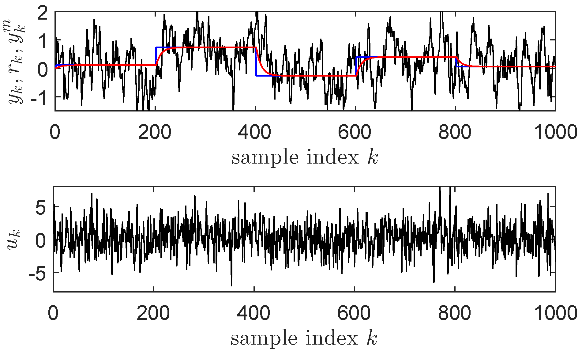
For data collection, the ORM’s output is collected along with: , and the reference input . The measurable extended state vector is then . A discretized version of an integral controller with t.f. at sampling period closes the loop of the control system and asymptotically stabilizes it, while calculating the control input based on the feedback error . This CS setup is used for collecting transition samples of the form . Data is collected for 500 s, with normally distributed random reference inputs having variance , modeled as piece-wise constant steps that change their values every 20 s. Normally distributed white noise having variance is added on the command at every time step to ensure a proper exploration by visiting as many combinations of states and actions as possible. Exploration has a critical role in the success of the IMF-AVI. A higher amplitude additive noise on increases the chances of converging the approximate VI approach. The state transitions data collection is shown in Figure 1 for the first 1000 samples (100 s).
Notice that a reference input modeled as a sequence of constant amplitude steps is used for exploration purposes, for which it may not be possible to write as a generative model. To solve this, all transition samples that correspond to the switching times of the reference input are eliminated, therefore, can be considered as the piece-wise constant generative model of the reference input.
The control objective is to minimize from (5) using the stage cost (where the outputs obviously depend on the extended states as per (31)), with the discount factor . Thus the overall objective is to find the optimal state-feedback controller that makes the feedback CS match the ORM.
The Q-function is linearly parameterized as , with the quadratic basis functions vector constructed by the unique terms of the Kronecker product of all input arguments of as
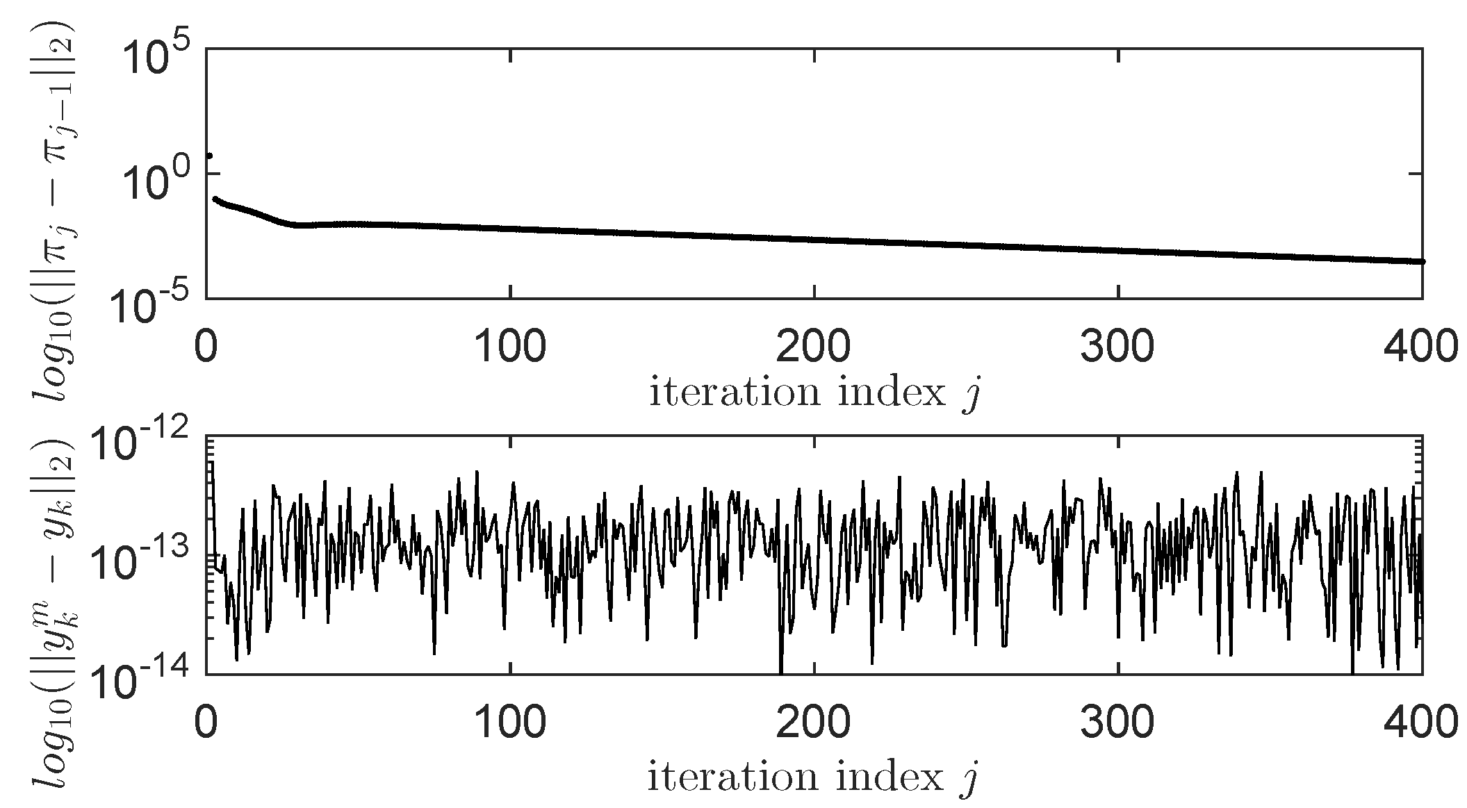
with . The controller improvement step equivalent to explicitly minimizing the Q-function w.r.t. the control input is . This improved linear-in-the-state controller is embedded in the linear system of equations (12) that is solved for every iteration of IMF-AVI. Each iteration produces a new that is tested on a test scenario where the uniformly random reference inputs have amplitude and switch every 10 s. The ORM tracking performance is then measured by the Euclidean vector norm while serves as a stopping condition when it drops below a prescribed threshold. The practically observed convergence process is shown in Figure 2 over the first 400 iterations, with still decreasing after 1000 iterations. While is very small right from the first iterations, making the process output practically overlap with the ORM’s output.
Comment 7.
For LTI processes with an LQR-like c.f., an LTI ORM and an LTI generative reference input model, linear parameterizations of the extended Q-function of the form is the well-known [9] form of the quadratic Q-function, with parameter being the vectorized form of the symmetric positive-definite matrix P and the basis function vector is obtained by the nonrepeatable terms of the Kronecker product of all the Q-function input arguments.
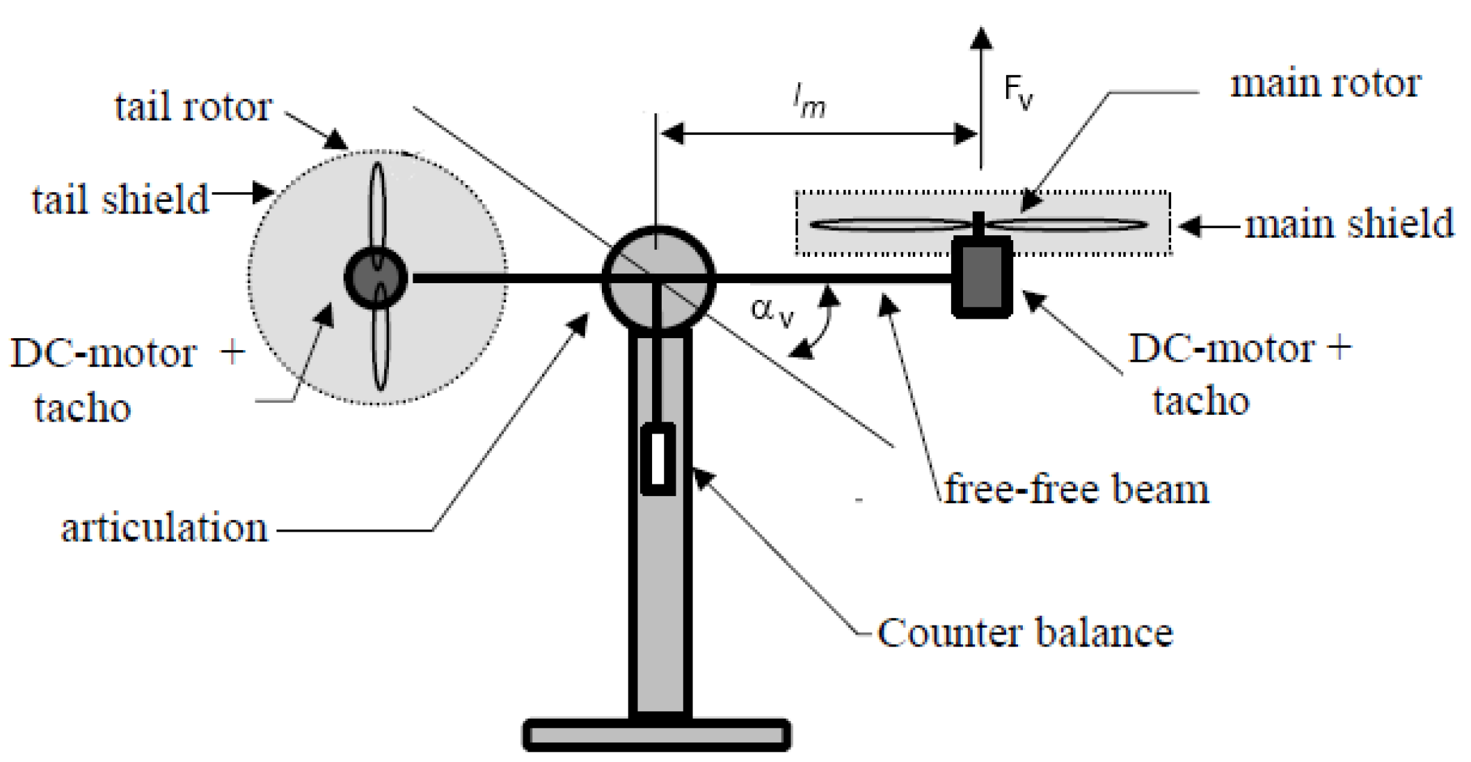
4.2. IMF-AVI on the Nonlinear TITOAS Aerodynamic System
The ORM tracking problem on the more challenging TITOAS angular position control [50] (Figure 3) is aimed next. The azimuth (horizontal) motion behaves as an integrator while the pitch (vertical) positioning is affected differently by the gravity for the up and down motions. Coupling between the two channels is present. A simplified deterministic continuous-time state-space model of this process is given as two coupled state-space sub-systems [12,46]:
where is the saturation function on , is the azimuth motion control input, is the vertical motion control input, is the azimuth angle output, is the pitch angle output, other states being described in [11,48]. The nonlinear static characteristics obtained by polynomial fitting from experimental data are for [46]:
A zero-order hold on the inputs and a sampler on the outputs of (33) lead to an equivalent MP discrete-time model of sampling time and of relative degree 1 (one), suitable for input-state data collection
where and . The process’ dynamics will not be used for learning the control in the following.
4.3. Initial Controller with Model-Free VRFT
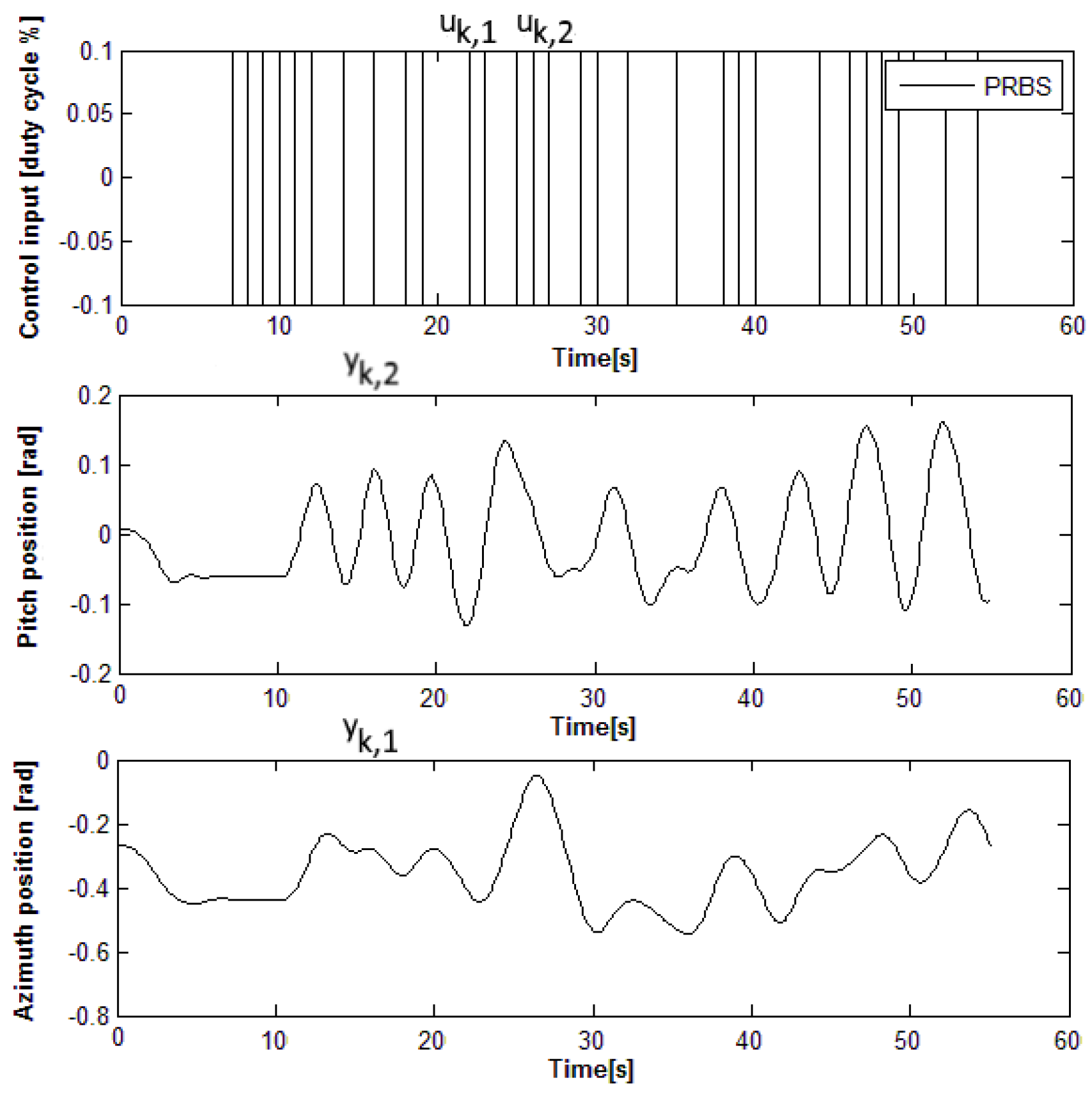
An initial model-free multivariable IO controller is first found using model-free VRFT, as described in [11,24,32]. The ORM is where are the discrete-time counterparts of obtained for a sampling period of s. The VRFT prefilter is chosen as . A pseudo-random binary signal (PRBS) of amplitude is used on both inputs to open-loop excite the pitch and azimuth dynamics simultaneously, as shown in Figure 4. The IO data is collected with low-amplitude zero-mean inputs , in order to maintain the process linearity around the mechanical equilibrium, such that to fit the linear VRFT design framework (© 2019 IEEE [12]).
An un-decoupling linear output feedback error diagonal controller with the parameters computed by the VRFT approach is [12,46]
where the parameter vector groups all the coefficients of . Controller (36) is obtained for as the least squares minimizer of where , . Here, is an approximation of the c.f. from (5) obtained for . The controller (36) will then close the feedback control loop as in .
Notice that, by formulation, the VRFT controller tuning aims to minimize the undiscounted () from (5), but via the output feedback controller (36) that processes the feedback control error . The same goal to minimize (5) is pursued by the subsequent IMF-AVI design of a state-feedback controller tuning for the extended process. Nonlinear (in particular, linear) state-feedback controllers can also be found by VRFT as shown in [24,32], to serve as initializations for the IMF-AVI, or possibly, even for PoIt-like algorithms. However, should this not be necessary, IO feedback controllers are much more data-efficient, requiring significantly less IO data to obtain stabilizing controllers.
4.4. Input–State–Output Data Collection
ORM tracking is intended by making the closed loop CS match the same ORM . With the linear controller (36) used in closed-loop to stabilize the process, input–state–output data is collected for 7000 s. The reference inputs with amplitudes model successive steps that switch their amplitudes uniformly random at 17 s and 25 s, respectively. On the outputs of both controllers , an additive noise is added at every 2nd sample as an uniform random number in for and in for . These additive disturbances provide an appropriate exploration, visiting many combinations of input–states–outputs. The computed controller outputs are saturated to , then sent to the process. The reference inputs drive the ORM [12,46]:
Then the states of the ORM (also outputs of the ORM) are also collected along with the states and control inputs of the process, to build the process extended state (4). Let the extended state be:
Essentially, the collected and builds the transitions dataset for , used for the IMF-AVI implementation. After collection, an important processing step is the data normalization. Some process states are scaled in order to ensure that all states are inside [−1;1]. The scaled process state is and . Other variables such as the reference inputs, the ORM states and the saturated process inputs already have values inside . The normalized state is eventually used for state feedback. Collected transition samples are shown in Figure 5 only for the process inputs and outputs, ORM’s outputs and reference inputs, for the first 400 s (4000 samples) out of 7000 s [12].
Note that the reference input signals used as sequences of constant amplitude steps for ensuring good exploration, do not have a generative model that obeys the Markov assumption. To avoid this problem, the piece-wise constant reference input generative model is employed by eliminating from the dataset D all the transition samples that correspond to switching reference inputs instants (i.e., when at least one of switches) (© 2019 IEEE [12]).
4.5. Learning State-Feedback Controllers with Linearly Parameterized IMF-AVI
Details of the LP-IMF-AVI applied to the ORM tracking control problem are next provided. The stage cost is defined and the discount factor in is . The Q-function is linearly parameterized using the basis functions [12]
This basis functions selection is inspired by the shape of the quadratic Q-function resulting from LTI processes with LQR-like penalties (see Comment 7). It is expected to be a sensible choice since the TITOAS process is a nonlinear one, therefore the quadratic Q-function may under-parameterize the true Q-function. Nevertheless, its computational advantage incentives the testing of such a solution. Notice that the controller improvement step at each iteration of the LP-IMF-AVI is based on explicit minimization of the Q-function. Solving the linear system of equations resulting after setting the derivative of w.r.t. equal to zero, it is obtained that (© 2019 IEEE [12])
The improved controller is embedded in the system (12) of 70,000 linear equations with 78 unknowns corresponding to the parameters of . This linear system (12) is solved in least squares sense, with each of the 50 iterations of the LP-IMF-AVI. The practical convergence results are shown in Figure 6 for and for the ORM tracking performance in terms of a normalized c.f. measured for samples over 200 s in the test scenario displayed in Figure 7. The test scenario consists of a sequence of piece-wise constant reference inputs that switch at different moments of time for the azimuth and pitch ( and , respectively), to illustrate the existing coupling behavior between the two control channels and the extent to which the learned controller manages to achieve the decoupled behavior requested but the diagonal ORM (© 2019 IEEE [12]).
The best LP-IMF-AVI controller found over the 50 iterations results in (tracking results in black lines in Figure 7) (© 2019 IEEE [12]), which is more than 6 times lower than the tracking performance of the VRFT controller used for transition samples collection, for which (tracking results in green lines in Figure 7). The convergence of the LP-IMF-AVI parameters is depicted in Figure 8.
4.6. Learning State-Feedback Controllers with Nonlinearly Parameterized IMF-AVI Using NNs
The previous LP-IMF-AVI for ORM tracking control learning scheme is next challenged by a NP-IMF-AVI implemented with NNs. In this case, two NNs are used to approximate the Q-function and the controller (the latter is sometimes avoidable, see the comments later on in this sub-section). The procedure follows the NP-IMF-AVI implementation described in [24,51]. The same dataset of transition samples is used as was previously used for the LP-IMF-AVI. Notice that the NN-based implementation is widely used in the reinforcement learning-based approach of ADP and is generally more scalable to problems of high dimension.
The controller NN (C-NN) estimate is a 10–3–2 (10 inputs because , 3 neurons in the hidden layer, and 2 outputs corresponding to ) with activation function in the hidden layer and linear output activation. The Q-function NN (Q-NN) estimate is 12–25–1 with the same parameters as C-NN. Initial weights of both NNs are uniform random numbers with zero-mean and variance 0.3. Both NNs are to be trained using scaled conjugate gradient for a maximum of 500 epochs. The available dataset is randomly divided into training (80%) and validation data (20%). Early stopping during training is enforced after 10 increases of the training c.f. mean sum of squared errors (MSE) evaluated on the validation data. MSE is herein, for all networks, the default performance function used in training (© 2019 IEEE [12]).
The NP-IMF-AVI proposed herein consists of two steps for each iteration j. The first one calculates the targets for the NN (having inputs and current iteration weights ) as , for all transitions in the dataset. Resulting in the trained Q-function estimator NN with parameter weights . The second step (the controller improvement) first calculates the targets for the controller (with inputs ) as . Note that additional parameterization for the controller NN weights is needed. Training produces the improved controller characterized by the new weights . Here, the discrete set of control actions used to minimize the Q-NN estimate for computing the controller targets is the Cartesian product of two identical sets of control actions, each containing 21 equally spaced values in [–1;1], i.e., .
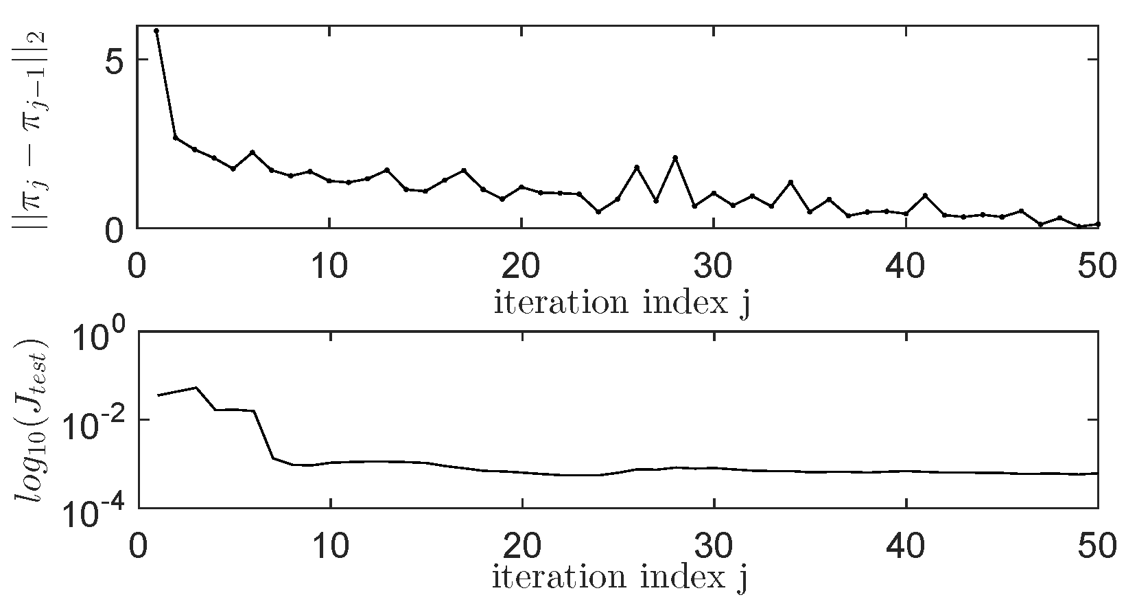
A discount will be used and each iteration of the NP-IMF-AVI produces a C-NN that is tested on the standard test scenario shown in Figure 6 by measuring the same normalized c.f. for , on the same test scenario that was used in the case of the LP-IMF-AVI. The NP-IMF-AVI is iterated 50 times and all the stabilizing controllers that are better than the VRFT multivariable controller running on the standard test scenario described in Figure 7 (in terms of smaller ) are stored. The best C-NN across 50 iterations renders . The tracking performance for the best NN controller found with the NP-IMF-AVI is shown in blue lines in Figure 7. The convergence process is depicted in Figure 9.
A gridsearch is next performed for the NP-IMF-AVI training process, by changing the dataset size from 30,000 to 50,000 to 70,000, combined with 17, 19, and 21 discrete values used for minimizing the Q-function over the two control inputs. For the case of 50,000 data with 17 uniform discrete possible values for each control input, which is the same with the best performance of the LP-IMF-AVI. Notice that neither the nonlinear state-feedback controller of the NP-IMF-AVI nor the linear state-feedback controller of the LP-IMF-AVI have integral component, while the linear output feedback controller tuned by VRFT and used for exploration has integrators.
Two additional approaches exist for dealing with a NP-IMF-AVI using two NNs, for each of the Q-NN approximator and for the C-NN. For example, [32] used to cascade the C-NN and the Q-NN. After training the Q-NN and producing the new weights , the weights of the Q-NN are fixed and only the weights of the C-NN are trained, with all the targets equal to for all the inputs of the cascaded NN . In this way, the C-NN is forced to minimize the Q-NN. The disadvantage is the vanishing gradient problem of the resulted cascaded network that deepens through more hidden layers, therefore only small corrections are brought to the C-NN part that is further away from the Q-NN’s output. Yet another solution [14] uses, for the controller improvement step, a single/several gradient descent step/steps with each iteration of NP-IMF-AVI, with step size and with gradient accumulated over all inputs of the cascaded NN , over fixed Q-NN weights. Essentially, the two approaches described above are equivalent and the number of gradient descent steps at each iteration is user-selectable. Also, no minimization by enumerating a finite set of control actions needs to be performed in either of the two above approaches. The above two equivalent approaches are effectively a particular case of the Neural-Fitted Q-iteration with Continuous Actions (NFQCA) approach [14], more recently to be updated with some changes to Deep Deterministic Policy Gradient (DDPG) [52]. DDPG uses two NNs as well, for the Q-NN and for the C-NN. It was originally developed to work in online off-policy mode, hence the need to update the Q-NN and the C-NN in a faster way on a relatively small number of transition samples (called minibatch) randomly extracted from a replay buffer equivalent to the dataset D, in order to break the time correlation of consecutive samples. The effectiveness of DDPG in real-time online control has yet to be proven.
Two variants of offline off-policy DDPG called DDPG1 and DDPG2 are run for comparisons purposes. Both use minibatches of 128 transitions from the dataset D at each training iteration. While both use soft target updates of the Q-NN weights and of the C-NN weights , with . and are used to calculate the targets for the Q-NN training. At each iteration, DDPG1 makes one update step of the Q-NN weights in the negative direction of the gradient of the MSE w.r.t. with step size and one update step of the C-NN weights in the negative direction of the gradient of the Q-NN’s output w.r.t. with step size . While DDPG2 differs in that the Q-NN training on each minibatch of each iteration is left to the same settings used for NP-IMF-AVI training (scaled conjugate gradient for maximum 500 epochs), only one gradient descent step is used to update the C-NN weights with the same . The step-sizes were selected to ensure learning convergence. It was observed that DDPG1 has the slowest convergence (convergence appears after more than 20,000 iterations) since it performs only one gradient update step per iteration, DDPG2 has faster convergence speed (convergence appears after 5000 iterations) since it allows more gradient steps for Q-NN training, while NP-IMF-AVI has the highest convergence speed (convergence appears after 10 iterations), allowing more training in terms of gradient descent steps (with scaled conjugate gradient direction) for both Q-NN and for C-NN, at each iteration. This proves that, given the high-dimensional process, it is better to use the entire dataset D for offline training, as it was done with NP-IMF-AVI. On the other hand, the best performance with DDPG1 and DDPG2 is 0.003, not as good as the best one with the more computationally demanding NP-IF-AVI (0.0017), suggesting that minimizing the Q-NN by enumerating discrete actions to calculate the C-NN targets may actually escape local minima. The total learning time to convergence with DDPG1 and DDPG2 is about the same as with NP-IMF-AVI, which is to be expected since less calculations for DDPG1 takes more iterations until convergence appears. Notice that NP-IMF-AVI does not use soft target updates for its two NNs.
The additional NN controller is not mandatory and the NP-IMF-AVI can be made similar to the LP-IMF-AVI case. In this case, the minimization of the Q-function NN estimate is to be performed by enumerating the discrete set of control actions and the targets calculation for the Q-function NN will use . This approach merges the controller improvement step and the Q-function improvement step. However, for real-time control implementation after NP-IMF-AVI convergence, it is more expensive to find , since it requires evaluating the Q-function NN for a number of times proportional to the number of combinations of discrete control actions. Then only slower processes can be accommodated with this implementation. Whereas in the case when a dedicated controller NN is used, after NP-IMF-AVI convergence, the optimal control is calculated at once, through a single NN evaluation. This dedicated NN controller can also be obtained (trained) as a final step after the NP-IMF-AVI has converged to the optimal Q-function and the targets for the controller output are calculated as . Another original solution that uses a single NN Q-function approximator was proposed in [53], such that a quadratic approximation of the NN-fitted Q-function is used to directly derive a linear state-feedback controller with each iteration.
4.7. Comments on the Obtained Results
Some comments follow the validation of the LP-IMF-AVI and NP-IMF-AVI. The results of Figure 6 indicate that convergence of the LP-IMF-AVI is attained in terms of , however perfect ORM tracking is not possible, as shown by the nonzero constant value of . On one hand, this is to be expected since the resulting linear state-feedback controller coupled with the process’ nonlinear dynamics is not capable of ensuring a closed-loop linear behavior as requested by the ORM. On the other hand, the NN controller resulting from the NP-IMF-AVI implementation is a nonlinear state feedback controller, however the best obtained results are not better than (but on the same level with) those obtained with the linear state-feedback controller of the NP-IMF-AVI, although the nonlinear controller is expected to perform better in terms of lower , due to its flexibility being able to compensate for the process nonlinearity. If this flexibility does not turn into an advantage, the reason lies with the additional NN controller parameterization (that introduces additional approximation errors) and with the training process that relies on approximate minimizations in the calculation step of the controller’s targets.
The iterative evolution of in case of both LP-IMF-AVI and NP-IMF-AVI show stabilization to constant nonzero values, suggesting that neither approach can provide perfectly ORM tracking controllers. For the LP-IMF-AVI, the responsibility lies with the under-representation error introduced by quadratic Q-function (and with the subsequent resulting linear state-feedback controller), while for NP-IMF-AVI, responsibility lies with the errors introduced by the additional controller approximator NN and the targets calculation in the controller improvement step.
Computational resources analysis indicate that the LP-IMF-AVI has learned only 78 parameters for to the Q-function parameterization, and no intermediate controller approximator is used. The run time for 50 iterations is about 345 seconds (including evaluation steps on the test scenario after each iteration). The NN-based NP-IMF-AVI needs to learn two NNs having 351 parameters (weights) for the Q-function NN and 41 parameters (weights) for the controller NN, respectively. Contrastingly, the runtime for the NP-IMF-AVI is about 3300 seconds, almost ten times more than in the case of the LP-IMF-AVI. Despite the larger parameter learning space, the converged behavior of the NN-based NP-IMF-AVI is very similar to that of the LP-IMF-AVI (see tracking results in Figure 7).
LP-IMF-AVI has shown an increased sensitivity to the transition samples dataset size: for fewer or more transition samples in the dataset, the LP-IMF-AVI diverges, under exactly the same exploration settings. But this divergence appears only after an initial convergence phase similar to that of Figure 6, and not from the very beginning. Whereas having fewer transition samples is intuitively disadvantageous for learning the true Q-function approximation, having a larger number of transition samples leading to divergence is unexpected. The reason is that non-uniform state-action space exploration affects the linear regression. Then, given a fixed dataset size, an increased amplitude of the additive disturbance used to stimulate exploration combined with a more often application of this disturbance (such as every 2nd sample) increases the convergence probability. These observations indicate again that the proposed linear parameterization using quadratic basis functions is insufficient for a correct representation of the true Q-function, thus failing the small approximation errors assumptions of Theorem 2. The connection between the convergence guarantees and the approximation errors have been analyzed in the literature [54,55,56,57].
In the light of the previous paragraph’s observations, the NN-based NP-IMF-AVI proves to be significantly more robust throughout the convergence process, both to various transition samples dataset sizes and to different exploration settings (disturbance amplitude and frequency of its application, how often the reference inputs switch during the transition samples collection phase, etc.). This may well pay off for the additional controller approximator NN and for the extra computation time since the chances of learning high performance controllers will depend less on the selection of the many parameters involved. Moreover, manual selection of the basis functions is unnecessary with the NN-based NP-IMF-AVI, while the over-parameterization is automatically managed by the NN training mechanism.
Data normalization is a frequently overlooked issue in ADP control but it is critical to successful design since it numerically affects both the regression solution in LP-IMF-AVI and the NN training in NP-IMF-AVI. A diagonal scaling matrix leads to the scaled extended state resulting in the extended state-space model that still preserves the MDP property.
5. Conclusions
This paper proves a functional design for an IMF-AVI ADP learning scheme dedicated to the challenging problem of ORM tracking control for a high-order real-world complex nonlinear process with unknown dynamics. The investigation revolves around a comparative analysis of a linear vs. a nonlinear parameterization of the IMF-AVI approach. Learning high performance state-feedback control under the model-free mechanism offered by IMF-AVI builds upon the input–states–outputs transition samples collection step that uses an initial exploratory linear output feedback controller that is also designed in a model-free setup using VRFT. From the practitioners’ viewpoint, the NN-based implementation of IMF-AVI is more appealing since it easily scales up with problem dimension and automatically manages the basis functions selection for the function approximators.
Future work attempts to validate the proposed design approach to more complex high-order nonlinear processes of practical importance.
Author Contributions
Conceptualization, M.-B.R.; methodology, M.-B.R.; software, T.L; validation, T.L.; formal analysis, M.-B.R.; investigation, T.L.; data curation, M.-B.R. and T.L.; writing–original draft preparation, M.-B.R. and T.L.; writing–review and editing, M.-B.R. and T.L.; supervision, M.-B.R.
Funding
This research received no external funding
Conflicts of Interest
The authors declare no conflict of interest.
References
- Radac, M.B.; Precup, R.E.; Petriu, E.M. Model-free primitive-based iterative learning control approach to trajectory tracking of MIMO systems with experimental validation. IEEE Trans. Neural Netw. Learn. Syst. 2015, 26, 2925–2938. [Google Scholar] [CrossRef]
- Sutton, R.S.; Barto, A.G. Reinforcement Learning: An Introduction; MIT Press: Cambridge, MA, USA, 1998. [Google Scholar]
- Bertsekas, D.P.; Tsitsiklis, J.N. Neuro-Dynamic Programming; Athena Scientific: Belmont, MA, USA, 1996. [Google Scholar]
- Wang, F.Y.; Zhang, H.; Liu, D. Adaptive dynamic programming: an introduction. IEEE Comput. Intell. Mag. 2009, 4, 39–47. [Google Scholar] [CrossRef]
- Lewis, F.; Vrabie, D.; Vamvoudakis, K.G. Reinforcement learning and feedback control: Using natural decision methods to design optimal adaptive controllers. IEEE Control Syst. Mag. 2012, 32, 76–105. [Google Scholar]
- Lewis, F.; Vrabie, D.; Vamvoudakis, K.G. Reinforcement learning and adaptive dynamic programming for feedback control. IEEE Circ. Syst. Mag. 2009, 9, 76–105. [Google Scholar] [CrossRef]
- Murray, J.; Cox, C.J.; Lendaris, G.G.; Saeks, R. Adaptive dynamic programming. IEEE Trans. Syst. Man Cybern. 2002, 32, 140–153. [Google Scholar] [CrossRef]
- Mnih, V.; Kavukcuoglu, K.; Silver, D.; Rusu, A.A.; Veness, J.; Bellemare, M.G.; Graves, A.; Riedmiller, M.; Fidjeland, A.K.; Ostrovski, G.; et al. Human-level control through deep reinforcement learning. Nature 2015, 518, 529–533. [Google Scholar] [CrossRef]
- Kiumarsi, B.; Lewis, F.L.; Naghibi-Sistani, M.B.; Karimpour, A. Optimal tracking control of unknown discrete-time linear systems using input–output measured data. IEEE Trans. Cybern. 2015, 45, 2270–2779. [Google Scholar] [CrossRef]
- Kiumarsi, B.; Lewis, F.L.; Modares, H.; Karimpour, A.; Naghibi-Sistani, M.B. Reinforcement Q-learning for optimal tracking control of linear discrete-time systems with unknown dynamics. Automatica 2014, 50, 1167–1175. [Google Scholar] [CrossRef]
- Radac, M.B.; Precup, R.E.; Roman, R.C. Model-free control performance improvement using virtual reference feedback tuning and reinforcement Q-learning. Int. J. Syst. Sci. 2017, 48, 1071–1083. [Google Scholar] [CrossRef]
- Lala, T.; Radac, M.B. Parameterized value iteration for output reference model tracking of a high order nonlinear aerodynamic system. In Proceedings of the 2019 27th Mediterranean Conference on Control and Automation (MED), Akko, Israel, 1–4 July 2019; pp. 43–49. [Google Scholar]
- Ernst, D.; Geurts, P.; Wehenkel, L. Tree-based batch mode reinforcement learning. J. Mach. Learn. Res. 2005, 6, 2089–2099. [Google Scholar]
- Hafner, R.; Riedmiller, M. Reinforcement learning in feedback control. Challenges and benchmarks from technical process control. Mach. Learn. 2011, 84, 137–169. [Google Scholar] [CrossRef]
- Zhao, D.; Wang, B.; Liu, D. A supervised actor critic approach for adaptive cruise control. Soft Comput. 2013, 17, 2089–2099. [Google Scholar] [CrossRef]
- Cui, R.; Yang, R.; Li, Y.; Sharma, S. Adaptive neural network control of AUVs with Control input nonlinearities using reinforcement learning. IEEE Trans. Syst. Man Cybern. 2017, 47, 1019–1029. [Google Scholar] [CrossRef]
- Xu, X.; Hou, Z.; Lian, C.; He, H. Online learning control using adaptive critic designs with sparse kernel machines. IEEE Trans. Neural Netw. Learn. Syst. 2013, 24, 762–775. [Google Scholar]
- He, H.; Ni, Z.; Fu, J. A three-network architecture for on-line learning and optimization based on adaptive dynamic programming. Neurocomputing 2012, 78, 3–13. [Google Scholar] [CrossRef]
- Modares, H.; Lewis, F.L.; Jiang, Z.P. H∞ Tracking control of completely unknown continuous-time systems via off-policy reinforcement learning. IEEE Trans. Neural Netw. Learn. Syst. 2015, 26, 2550–2562. [Google Scholar] [CrossRef]
- Li, J.; Modares, H.; Chai, T.; Lewis, F.L.; Xie, L. Off-policy reinforcement learning for synchronization in multiagent graphical games. IEEE Trans. Neural Netw. Learn. Syst. 2017, 28, 2434–2445. [Google Scholar] [CrossRef]
- Bertsekas, D. Value and policy iterations in optimal control and adaptive dynamic programming. IEEE Trans. Neural Netw. Learn. Syst. 2017, 28, 500–509. [Google Scholar] [CrossRef]
- Yang, Y.; Wunsch, D.; Yin, Y. Hamiltonian-driven adaptive dynamic programming for continuous nonlinear dynamical systems. IEEE Trans. Neural Netw. Learn. Syst. 2017, 28, 1929–1940. [Google Scholar] [CrossRef]
- Kamalapurkar, R.; Andrews, L.; Walters, P.; Dixon, W.E. Model-based reinforcement learning for infinite horizon approximate optimal tracking. IEEE Trans. Neural Netw. Learn. Syst. 2017, 28, 753–758. [Google Scholar] [CrossRef]
- Radac, M.B.; Precup, R.E. Data-driven MIMO Model-free reference tracking control with nonlinear state-feedback and fractional order controllers. Appl. Soft Comput. 2018, 73, 992–1003. [Google Scholar] [CrossRef]
- Campi, M.C.; Lecchini, A.; Savaresi, S.M. Virtual Reference Feedback Tuning: A direct method for the design of feedback controllers. Automatica 2002, 38, 1337–1346. [Google Scholar] [CrossRef]
- Hjalmarsson, H. Iterative Feedback Tuning—An overview. Int. J. Adapt. Control Signal Process. 2002, 16, 373–395. [Google Scholar] [CrossRef]
- Janssens, P.; Pipeleers, G.; Swevers, J.L. Model-free iterative learning control for LTI systems and experimental validation on a linear motor test setup. In Proceedings of the 2011 American Control Conference (ACC), San Francisco, CA, USA, 29 June–1 July 2011; pp. 4287–4292. [Google Scholar]
- Radac, M.B.; Precup, R.E. Optimal behavior prediction using a primitive-based data-driven model-free iterative learning control approach. Comput. Ind. 2015, 74, 95–109. [Google Scholar] [CrossRef]
- Chi, R.; Hou, Z.S.; Jin, S.; Huang, B. An improved data-driven point-to-point ILC using additional on-line control inputs with experimental verification. IEEE Trans. Syst. Man Cybern. 2017, 49, 687–696. [Google Scholar] [CrossRef]
- Abouaissa, H.; Fliess, M.; Join, C. On ramp metering: towards a better understanding of ALINEA via model-free control. Int. J. Control 2017, 90, 1018–1026. [Google Scholar] [CrossRef]
- Hou, Z.S.; Liu, S.; Tian, T. Lazy-learning-based data-driven model-free adaptive predictive control for a class of discrete-time nonlinear systems. IEEE Trans. Neural Netw. Learn. Syst. 2017, 28, 1914–1928. [Google Scholar] [CrossRef]
- Radac, M.B.; Precup, R.E.; Roman, R.C. Data-driven model reference control of MIMO vertical tank systems with model-free VRFT and Q-learning. ISA Trans. 2018, 73, 227–238. [Google Scholar] [CrossRef]
- Bolder, J.; Kleinendorst, S.; Oomen, T. Data-driven multivariable ILC: enhanced performance by eliminating L and Q filters. Int. J. Robot. Nonlinear Control 2018, 28, 3728–3751. [Google Scholar] [CrossRef]
- Wang, Z.; Lu, R.; Gao, F.; Liu, D. An indirect data-driven method for trajectory tracking control of a class of nonlinear discrete-time systems. IEEE Trans. Ind. Electron. 2017, 64, 4121–4129. [Google Scholar] [CrossRef]
- Pandian, B.J.; Noel, M.M. Control of a bioreactor using a new partially supervised reinforcement learning algorithm. J. Proc. Control 2018, 69, 16–29. [Google Scholar] [CrossRef]
- Diaz, H.; Armesto, L.; Sala, A. Fitted q-function control methodology based on takagi-sugeno systems. IEEE Trans. Control Syst. Tech. 2018. [Google Scholar] [CrossRef]
- Wang, W.; Chen, X.; Fu, H.; Wu, M. Data-driven adaptive dynamic programming for partially observable nonzero-sum games via Q-learning method. Int. J. Syst. Sci. 2019. [Google Scholar] [CrossRef]
- Mu, C.; Zhang, Y. Learning-based robust tracking control of quadrotor with time-varying and coupling uncertainties. IEEE Trans. Neural Netw. Learn. Syst. 2019. [Google Scholar] [CrossRef] [PubMed]
- Liu, D.; Yang, G.H. Model-free adaptive control design for nonlinear discrete-time processes with reinforcement learning techniques. Int. J. Syst. Sci. 2018, 49, 2298–2308. [Google Scholar] [CrossRef]
- Song, F.; Liu, Y.; Xu, J.X.; Yang, X.; Zhu, Q. Data-driven iterative feedforward tuning for a wafer stage: A high-order approach based on instrumental variables. IEEE Trans. Ind. Electr. 2019, 66, 3106–3116. [Google Scholar] [CrossRef]
- Kofinas, P.; Dounis, A. Fuzzy Q-learning agent for online tuning of PID controller for DC motor speed control. Algorithms 2018, 11, 148. [Google Scholar] [CrossRef]
- Radac, M.-B.; Precup, R.-E. Three-level hierarchical model-free learning approach to trajectory tracking control. Eng. Appl. Artif. Intell. 2016, 55, 103–118. [Google Scholar] [CrossRef]
- Radac, M.-B.; Precup, R.-E. Data-based two-degree-of-freedom iterative control approach to constrained non-linear systems. IET Control Theory Appl. 2015, 9, 1000–1010. [Google Scholar] [CrossRef]
- Salgado, M.; Clempner, J.B. Measuring the emotional state among interacting agents: A game theory approach using reinforcement learning. Expert Syst. Appl. 2018, 97, 266–275. [Google Scholar] [CrossRef]
- Silva, M.A.L.; de Souza, S.R.; Souza, M.J.F.; Bazzan, A.L.C. A reinforcement learning-based multi-agent framework applied for solving routing and scheduling problems. Expert Syst. Appl. 2019, 131, 148–171. [Google Scholar] [CrossRef]
- Radac, M.-B.; Precup, R.-E.; Hedrea, E.-L.; Mituletu, I.-C. Data-driven model-free model-reference nonlinear virtual state feedback control from input-output data. In Proceedings of the 2018 26th Mediterranean Conference on Control and Automation (MED), Zadar, Croatia, 19–22 June 2018; pp. 332–338. [Google Scholar]
- Campestrini, L.; Eckhard, D.; Gevers, M.; Bazanella, M. Virtual reference tuning for non-minimum phase plants. Automatica 2011, 47, 1778–1784. [Google Scholar] [CrossRef]
- Al-Tamimi, A.; Lewis, F.L.; Abu-Khalaf, M. Discrete-time nonlinear HJB Solution using approximate dynamic programming: Convergence proof. IEEE Trans. Syst. Man Cybern. Cybern. 2008, 38, 943–949. [Google Scholar] [CrossRef] [PubMed]
- Rantzer, A. Relaxed dynamic programming in switching systems. IEEE Proc. Control Theory Appl. 2006, 153, 567–574. [Google Scholar] [CrossRef] [Green Version]
- Inteco, LTD. Two Rotor Aerodynamical System; User’s Manual; Inteco, LTD: Krakow, Poland, 2007; Available online: http://ee.sharif.edu/~lcsl/lab/Tras_um_PCI.pdf (accessed on 12 June 2019).
- Radac, M.-B.; Precup, R.-E. Data-driven model-free slip control of anti-lock braking systems using reinforcement Q-learning. Neurocomputing 2018, 275, 317–329. [Google Scholar] [CrossRef]
- Lillicrap, T.P.; Hunt, J.J.; Pritzel, A.; Heess, N.; Erez, T.; Tassa, Y.; Silver, D.; Wierstra, D. Continuous control with deep reinforcement learning. Mach. Learn. 2016, arXiv:1509.02971. [Google Scholar]
- Ten Hagen, S.; Krose, B. Neural Q-learning. Neural Comput. Appl. 2003, 12, 81–88. [Google Scholar] [CrossRef]
- Radac, M.B.; Precup, R.E. Data-Driven model-free tracking reinforcement learning control with VRFT-based adaptive actor-critic. Appl. Sci. 2019, 9, 1807. [Google Scholar] [CrossRef]
- Dierks, T.; Jagannathan, S. Online optimal control of affine nonlinear discrete-time systems with unknown internal dynamics by using time-based policy update. IEEE Trans. Neural Netw. Learn. Syst. 2012, 23, 1118–1129. [Google Scholar] [CrossRef]
- Heydari, A. Theoretical and numerical analysis of approximate dynamic programming with approximation errors. J. Gui Control Dyn. 2016, 39, 301–311. [Google Scholar] [CrossRef]
- Heydari, A. Revisiting approximate dynamic programming and its convergence. IEEE Trans. Cybern. 2014, 44, 2733–2743. [Google Scholar] [CrossRef] [PubMed]
Figure 1.
Closed-loop state transitions data collection for Example 1: (top) (black), (blue), (red); (bottom) .
Figure 1.
Closed-loop state transitions data collection for Example 1: (top) (black), (blue), (red); (bottom) .

Figure 2.
Convergence results of the linearly paramaterized iterative model-free approximate Value Iteration (LP-IMF-AVI) for the linear process example.
Figure 2.
Convergence results of the linearly paramaterized iterative model-free approximate Value Iteration (LP-IMF-AVI) for the linear process example.

Figure 3.
The two-inputs–two-outputs aerodynamic system (TITOAS) experimental setup.

Figure 4.
Open-loop input–output (IO) data from the two-inputs–two-outputs aerodynamic system (TITOAS) for Virtual Reference Feedback Tuning (VRFT) controller tuning [46].
Figure 4.
Open-loop input–output (IO) data from the two-inputs–two-outputs aerodynamic system (TITOAS) for Virtual Reference Feedback Tuning (VRFT) controller tuning [46].

Figure 5.
IO data collection with the linear controller: (a) ; (b) (black), (red), (black dotted); (c) ; (d) (black), (red), (black dotted).
Figure 5.
IO data collection with the linear controller: (a) ; (b) (black), (red), (black dotted); (c) ; (d) (black), (red), (black dotted).

Figure 6.
The LP-IMF-AVI convergence on TITOAS (© 2019 IEEE [12]).
Figure 6.
The LP-IMF-AVI convergence on TITOAS (© 2019 IEEE [12]).

Figure 7.
The IMF-AVI convergence on TITOAS: , (red); for LP-IMF-AVI (black), for NP-IMF-AVI with NNs (blue), for the initial VRFT controller used for transitions collection (green) (© 2019 IEEE [12]).
Figure 7.
The IMF-AVI convergence on TITOAS: , (red); for LP-IMF-AVI (black), for NP-IMF-AVI with NNs (blue), for the initial VRFT controller used for transitions collection (green) (© 2019 IEEE [12]).

Figure 8.
The LP-IMF-AVI parameters convergence.

Figure 9.
The nonlinearly parameterized IMF-AVI (NP-IMF-AVI) convergence.

© 2019 by the authors. Licensee MDPI, Basel, Switzerland. This article is an open access article distributed under the terms and conditions of the Creative Commons Attribution (CC BY) license (http://creativecommons.org/licenses/by/4.0/).
Share and Cite
MDPI and ACS Style
Radac, M.-B.; Lala, T. Learning Output Reference Model Tracking for Higher-Order Nonlinear Systems with Unknown Dynamics. Algorithms 2019, 12, 121. https://doi.org/10.3390/a12060121
AMA Style
Radac M-B, Lala T. Learning Output Reference Model Tracking for Higher-Order Nonlinear Systems with Unknown Dynamics. Algorithms. 2019; 12(6):121. https://doi.org/10.3390/a12060121
Chicago/Turabian StyleRadac, Mircea-Bogdan, and Timotei Lala. 2019. "Learning Output Reference Model Tracking for Higher-Order Nonlinear Systems with Unknown Dynamics" Algorithms 12, no. 6: 121. https://doi.org/10.3390/a12060121
Note that from the first issue of 2016, this journal uses article numbers instead of page numbers. See further details here.