Integration of Production Planning and Scheduling Based on RTN Representation under Uncertainties

Abstract

Production planning and scheduling are important bases for production decisions. Concerning the traditional modeling of production planning and scheduling based on Resource-Task Network (RTN) representation, uncertain factors such as utilities are rarely considered as constraints. For the production planning and scheduling problem based on RTN representation in an uncertain environment, this paper formulates the multi-period bi-level integrated model of planning and scheduling, and introduces the uncertainties of demand and utility in planning and scheduling layers respectively. Rolling horizon optimization strategy is utilized to solve the bi-level integrated model iteratively. The simulation results show that the proposed model and algorithm are feasible and effective, can calculate the consumption of utility in every period, decrease the effects of uncertain factors on optimization results, more accurately describe the uncertain factors, and reflect the actual production process.

1. Introduction

Production planning and scheduling are important bases for production decisions, and play an important role in economic benefits. In the traditional control of production processes, production planning and scheduling are optimized, respectively, which has obvious disadvantages such as the infeasibility and sub-optimality of optimization results. With the rapid development of economic globalization and product demand diversification, competition among enterprises is more and more fierce. In order to arrange production reasonably and enhance competitiveness of enterprises, enterprise managers and researchers realize that single production planning or scheduling cannot satisfy the needs of production and management in enterprises. Consequently, the integration problem of production planning and scheduling is receiving more and more attention [1] in the complex and changeable economic situation [2,3].

Shao et al. [4] proposed that production planning and scheduling are complementary, and that integration of production planning and scheduling can enhance the performance of production management greatly. Lasserre [5] formulated a holistic integrated model of production planning and scheduling, and solved the integrated model hierarchically. Xiong et al. [6] explored multi-period multi-workshop production planning and scheduling problems, and formulated an integrated optimization model of the production planning and scheduling based on nonlinear mixed integer programming. An alternant iterative method by hybrid genetic algorithm is employed to solve the integrated model, which promoted the research of the integration problem of production planning and scheduling. Li et al. [7] stated that implementing integrated optimization of planning and scheduling can improve the quality of decision making in the process operations, and also proposed a new decomposition strategy based on two-level optimization. Wang et al. [8] formulated a bi-level integrated model of production planning and scheduling based on State-Task Network (STN) representation, and introduced the rolling horizon optimization strategy to solve the bi-level integrated model iteratively. The feasibility and effectiveness of the proposed model are illustrated through benchmark examples. Vogel et al. [9] developed a hierarchical and integrated model considering both levels, aggregate production planning, and master production scheduling. Computational tests show that it is possible to solve the integrated model and it outperforms the existing hierarchical approach for all instances. Hassani et al. [10] proposed a new model integrating planning and scheduling to make up for the defect that the capacity limitation could not reflect the practical availability of resources, and added the constraint of resource availability. In this model, the optimization total cost of a single-level job shop was taken as the objective function, and the random approximation method was adopted as the genetic algorithm to solve the N-P problem.

A reasonable and elaborate representation for production processes is an important point to establish production planning and scheduling model. In the process industry, general representation methods for production process include STN, State-Sequence Network (SSN) and Resource-Task Network (RTN). Pantelides et al. [11] proposed the RTN representation method, which is a comprehensive and concise process-representation method. This representation method can describe all the resource properties in a unified manner. Any kinds of facilities and other resources are not distinctive, and considered as producible and consumable resources when the tasks are active. Zhang et al. [12] extended the concept of RTN to provide a unified mathematical formulation of the problem of determining the optimal operating conditions of a mixed production facility, comprising a multipurpose plant for both batch and continuous operations. Alternative approaches for solving the general problem were discussed, and some preliminary numerical results were presented. Castro et al. [13] proposed an improved general mathematical programming formulation for optimal scheduling of batch processes based on the RTN representation. The proposed models led to simpler and less degenerate mathematical models. These models can be solved in significantly less CPU time, when compared to other RTN continuous-time formulations. Chen et al. [14] proposed an improved mixed integer linear programming model for short-term scheduling of multipurpose batch plants under maximization of profit based on RTN representation and unit-specific events. To solve the model, a hybrid method based on line-up competition algorithm and linear programming was presented. Simulation results show that the proposed model and hybrid method were effective for short-term scheduling of multipurpose batch plants. Some research achievements on the production planning and scheduling problem based on RTN representation were proposed, however, the majority of these achievements are under determinate condition, and do not involve uncertain factors [15,16]. Chao et al. [17] believed that distributionally robust optimization (DRO) is a new and effective method to deal with the imprecise probability distribution of uncertain parameters in the decision-making process. They proposed an effective DRO framework to solve the production planning and scheduling problem in the uncertain demand environment. Based on this, they considered the multi-stage sequential decision structure in the operation process. Curcio et al. [18] proposed an adaptive strategy applicable to the multi-stage setting of the two-stage planning and robust optimization model, and an approximate heuristic algorithm based on multistage stochastic programming and adjustable robust optimization. The simulation results show that the strategies are promising in solving large-scale problems: the approximate strategy based on adjustable robust optimization has, on average, 6.72% better performance and is 7.9 times faster than the deterministic model. Production planning and scheduling problem based on RTN representation considering uncertain factors as constraints in production process, is rare. This paper formulates the multi-period bi-level integrated model of production planning and scheduling, considers the demand and utility uncertainties for the production planning and scheduling problem based on RTN presentation. A deterministic model with two layers of planning and scheduling is formulated firstly. In the deterministic model, uncertainties of demand and utility are treated as deterministic parameters in the planning layer and scheduling layer respectively. Then the chance constrained programming [19] and fuzzy theory [20,21] are introduced into the planning layer model and scheduling layer model, respectively, to describe the uncertainties of demand and utility [22,23]. The planning layer model is formulated by the discrete-time modeling method [24]. The scheduling layer model is formulated by the unit-specific event-based continuous-time modeling method. Rolling horizon optimization strategy [25] is utilized to solve the bi-level integrated model iteratively. The simulation results show that the model and algorithm can accurately describe the uncertain factors, decrease the effects of uncertain factors on optimization results, and more accurately reflect the actual production processes.

This paper is organized as follows: Section 1 introduces the research status of production planning and scheduling integration. Section 2 establishes the deterministic model and the uncertain model at the planning layer and the scheduling layer respectively. Section 3 introduces the rolling horizon optimization strategy. An example is simulated and analyzed in Section 4. Conclusions are presented in Section 5.

2. Mathematical Model

2.1. Planning Layer Model

Due to the long time scale of the planning layer, it can be divided evenly into several time periods. A discrete-time linear programming model is established at the planning layer, with the maximization of profits as the objective function. Chance constrained programming is introduced to describe the uncertainty of demand. Through a series of mathematical transformations, the uncertain model with chance constraints is transformed into a deterministic model with a specified confidence level. At last, the transformed deterministic model is solved.

2.1.1. Deterministic Model

1. Objective function:

$$max{\displaystyle \sum _{i\in G_p}{\displaystyle \sum _{k\in K}\left[Pric{e}_i\cdot D(i,k)-\alpha \cdot Pric{e}_i\cdot Td(i,k)-\beta \cdot Flu(i,k)-\theta \cdot Inv(i,k)\right]}}.$$

(1)

The maximum of profit is taken as the objective function of the production planning layer model, where the first part represents the product profit, the second part represents the punishment cost caused by the backlog order quantity of the products, the third part represents the cost paid due to the impact of the productivity fluctuation in the production processes, and the fourth part represents the cost paid when the inventory quantity exceeds the safe limit of inventory.

2. Material balance constraints:

$$S(i,k)=S(i,k-1)+P(i,k)-D(i,k)-{\displaystyle \sum _{j\in N_i}{c}_{ij}}\cdot P(j,k);i\in G_{all},k>1,k\in K.$$

(2)

$$S(i,k)=S_i^{ini}+P(i,k)-D(i,k)-{\displaystyle \sum _{j\in N_i}{c}_{ij}}\cdot P(j,k);i\in G_{all},k=1,k\in K.$$

(3)

Constraints (2) and (3) respectively represent the material balance in the subsequent period and the initial period. The inventory $s(i,k)$ of the material status $i$ at the end of the planning period $k$ is equal to the inventory at the end of the previous period $s(i,k-1)$ plus the output of current period $p(i,k)$, and finally minus the delivery of current period $D(i,k)$ and the corresponding consumption ${\displaystyle \sum _{j\in N_i}{c}_{ij}}\cdot P(j,k)$, which is consumed by downstream production. Among them, $N_i$ is the downstream material set of material state $i$; $c_{ij}$ is the conversion coefficient between material state $i$ and material state $j$.

3. Demand constraints:

$$Td(i,k)=Td(i,k-1)+Or{d}_{ik}-D(i,k);i\in G_p,k>1,k\in K.$$

(4)

$$D(i,k)\le Or{d}_{ik}+Td(i,k-1)+t{d}_{i,k};i\in G_p,k>1,k\in K.$$

(5)

Constraint (4) represents that the backlog order quantity $Td(i,k)$ of product $i$ in the period $k$ is equal to the backlog order quantity in the previous period $Td(i,k-1)$ plus the order quantity in the current period $Or{d}_{ik}$, minus the final delivery $D(i,k)$. In Constraint (5), $t{d}_{i,k}$ is a parameter in the model and, as a backlog order quantity generated by the scheduling layer, feedback to the next planning period, where, the delivery quantity $D(i,k)$ should be less than or equal to the sum of the order quantity of this period and backlog order quantity of the previous period, as well as the backlog order quantity from the scheduling layer in the previous period.

4. Production Capacity and Productivity Fluctuation Constraints:

$$P_i^{\min }\le P(i,k)\le P_i^{\max };i\in G_{ip},k\in K.$$

(6)

$$P(i,k)-Flu(i,k)\le P(i,k-1)\le P(i,k)+Flu(i,k);i\in G_{ip},k>1,k\in K.$$

(7)

Constraint (6) represents the production capacity constraint of materials. Material status $i$ produced in the period $k$ should be between maximum production capacity $P_i^{\max }$ and the minimum production capacity $P_i^{\min }$. In order to avoid excessive fluctuation of productivity in the adjacent periods, auxiliary variable $Flu(i,k)$ is introduced into Constraint (7) and corresponding penalty weight $\beta$ is introduced into the objective function, so as to reduce the loss caused by productivity fluctuation as much as possible.

5. Inventory constraints:

$$S_i^{\min }\le S(i,k)\le S_i^{\max };i\in G_{ip},k\in K.$$

(8)

$$S_i^{Ll}-Inv(i,k)\le S(i,k)\le S_i^{Ul}+Inv(i,k);i\in G_{ip},k\in K.$$

(9)

Constraint (8) represents the inventory of material status $i$ at the end of the period $k$. $S(i,k)$ should be between the inventory upper limit $S_i^{\max }$ and the inventory lower limit $S_i^{\min }$. In order to avoid the situation that the inventory storage level is too high or too low, auxiliary variable $Inv(i,k)$ is introduced into Constraint (9), and penalty weight $\theta$ is introduced into the corresponding objective function. The reference upper limit $S_i^{Ul}$ and lower limit $S_i^{Ll}$ of the inventory storage are set, so as to reduce the impact of the inventory storage level on the production processes.

2.1.2. Chance Constrained Uncertain Model

The uncertain factors in production planning have attracted more and more attention from scholars and researchers, as well as many methods and theories have been proposed to deal with the uncertain factors in production planning, including stochastic programming [26], fuzzy programming [27], robust optimization [28,29], recoverable robustness [30], sensitivity analysis [31] etc. At present, many research results have been obtained by using stochastic programming to deal with the problem of demand uncertainty [32,33]. Chance constrained programming is an important branch of stochastic programming. It allows decisions, to some extent, to not meet the constraints, but these decisions should make the probability of the constraints set up no less than a certain confidence level. The chance constrained method can more truly and effectively respond to demand uncertainty in the production planning.

The deterministic planning model is replaced by the following uncertainty planning model:

Objective function:(1)

Constraints: (2), (3), (6)–(9)

Constraint (10), deterministic constraint (4) is replaced by uncertainty constraint (10)

Constraint (11), deterministic constraint (5) is replaced by uncertainty constraint (11).

$$Td(i,k)=Td(i,k-1)+\tilde{O}r{d}_{ik}-D(i,k);i\in G_p,k>1,k\in K.$$

(10)

$$D(i,k)\le \tilde{O}r{d}_{ik}+Td(i,k-1)+t{d}_{i,k};i\in G_p,k>1,k\in K.$$

(11)

In Constraints (10) and (11), the parameter order demand quantity $\tilde{O}r{d}_{ik}$ is a random variable, assuming that the parameter obeys normal distribution, namely $N(E\left\{\tilde{O}r{d}_{ik}\right\},var\left\{\tilde{O}r{d}_{ik}\right\})$. Under a certain confidence level, Constraints (10) and (11) can be rewritten into Constraints (12) and (13).

$$Pr\left\{\tilde{O}r{d}_{ik}\ge D(i,k)+Td(i,k)-Td(i,k-1)\right\}\ge \lambda ;i\in G_p.$$

(12)

$$Pr\left\{\tilde{O}r{d}_{ik}\ge D(i,k)-Td(i,k-1)-t{d}_{i,k-1}\right\}\ge \beta ;i\in G_{p}k\in K.$$

(13)

By using the knowledge of Theorem 1 and Theorem 2 the probability density function can be used to further transform Constraints (12) and (13) into Constraints (14) and (15), and finally transform the model with demand uncertainty into a deterministic model with a confidence level. This transformation of the chance constraint has been solved in detail in many related studies [34,35], and it will not be repeated here in this paper.

$$\frac{\left[D(i,k)+Td(i,k)-Td(i,k-1)\right]-E\left\{Or{d}_{ik}\right\}}{\sqrt{var\left\{Or{d}_{ik}\right\}}}\le {\mathsf{\Phi }}^{-1}(i-\lambda );i\in G_p.$$

(14)

$$\frac{\left[D(i,k)-Td(i,k-1)-t{d}_{i,k-1}\right]-E\left\{Or{d}_{ik}\right\}}{\sqrt{var\left\{Or{d}_{ik}\right\}}}\le {\mathsf{\Phi }}^{-1}(i-\beta );i\in G_{p}k\in K.$$

(15)

Theorem 1.

For the random linear programming model:

$$\begin{array}{l}minZ={\displaystyle \sum _{j=1}^n{h}_j}•x_j;\\ s.t.\{\begin{array}{l}{\displaystyle \sum _{j=1}^n{g}_{ij}}•x_j\le {\mathrm{r}}_i(\xi \left)\right(i=1,2,\cdots ,m),\\ x_j\ge 0(j=1,2,\cdots ,n).\end{array}\end{array}$$

(16)

${\mathrm{r}}_i(\xi \left)\right(i=1,2,\cdots ,m)$is a single random variable, and the deterministic programming model with the formula at the confidence level$\nu$is as follows:

$$\begin{array}{l}minZ={\displaystyle \sum _{j=1}^n{h}_j}•x_j;\\ s.t.\{\begin{array}{l}{\displaystyle \sum _{j=1}^n{g}_{ij}}•x_j\le K_{\nu }^i(i=1,2,\cdots ,m),\\ x_j\ge 0(j=1,2,\cdots ,n).\end{array}\end{array}$$

(17)

In the formula,$K_{\nu }^i=sup\{K^i|K^i=F_i^{-1}(1-\nu )\},$$F_i(•)$is${\mathrm{r}}_i(\xi )$distribution function.

Theorem 2.

For the random linear programming model:

$$\begin{array}{l}minZ={\displaystyle \sum _{j=1}^n{h}_j}•x_j;\\ s.t.\{\begin{array}{l}{\displaystyle \sum _{j=1}^n{g}_{ij}}•x_j\ge {\mathrm{r}}_i(\xi \left)\right(i=1,2,\cdots ,m),\\ x_j\ge 0(j=1,2,\cdots ,n).\end{array}\end{array}$$

(18)

${\mathrm{r}}_i(\xi \left)\right(i=1,2,\cdots ,m)$is a single random variable, and the deterministic programming model with the formula at the confidence level$\nu$is as follows:

$$\begin{array}{l}minZ={\displaystyle \sum _{j=1}^n{h}_j}•x_j;\\ s.t.\{\begin{array}{l}{\displaystyle \sum _{j=1}^n{g}_{ij}}•x_j\ge K_{\nu }^i(i=1,2,\cdots ,m),\\ x_j\ge 0(j=1,2,\cdots ,n).\end{array}\end{array}$$

(19)

In the formula,$K_{\nu }^i=inf\{K^i|K^i=F_i^{-1}(\nu )\},$$F_i(•)$is${\mathrm{r}}_i(\xi )$distribution function.

2.2. Scheduling Layer Model

The continuous-time modeling method was adopted to establish the scheduling layer model. The optimization objective of the scheduling layer is to complete the production tasks assigned from the planning layer as much as possible. Therefore, the minimization of the value of the difference between the task amount assigned by the planning layer and the task amount completed by the scheduling layer was taken as the objective function. Resource balance constraint, capacity constraint, demand constraint, time constraint, sequence constraint, utility supply and utility time constraint were also considered. In scheduling layer, fuzzy theory is utilized to describe the uncertainty of the utility. Finally, the uncertainty model of utility is transformed into a deterministic model with membership degree by corresponding mathematical method.

2.2.1. Deterministic Model

1. Objective function:

$$minDe{f}_{r,k}-{\displaystyle \sum _{n\in N}d(r,n)};k\in K,r\in R^s.$$

(20)

The objective function is the minimization of the value of the difference between the task quantity assigned by the planning layer and the task quantity completed by the scheduling layer. The first part represents the reference task quantity assigned at the end of the planning period, and the second part represents the total final delivery of products completed by the scheduling layer within the planning period.

2. Resource balance constraints:

$$\begin{array}{l}E(r,n)=E(r,n-1)+{\displaystyle \sum _{i\in I_r}\left[{\mu }_{ri}^p\cdot w(i,n-1)+{\rho }_{ri}^p\cdot b(i,n-1)\right]}+{\displaystyle \sum _{i\in I_r}\left[{\mu }_{ri}^c\cdot w(i,n)+{\rho }_{ri}^c\cdot b(i,n)\right]};\\ r\in R,n>1,n\in N.\end{array}$$

(21)

$$E(r,n)=E_{ini}+{\displaystyle \sum _{i\in I_r}\left[{\mu }_{ri}^c\cdot w(i,n)+{\rho }_{ri}^c\cdot b(i,n)\right]};r\in R,n=1.$$

(22)

Constraints (21) and (22) respectively represent resource balance constraints of subsequent event points and the initial event point. The amount of available resources at event $n$ $E(r,n)$ is equal to the amount of available resources at the previous event point $E(r,n-1)$ plus the production amount of the previous event point, and the consumption of the current point. Moreover, in Constraints (21) and (22), ${\mu }_{ri}^c\le 0$, ${\rho }_{ri}^c\le 0$.

3. Capacity constraints:

$$E_r^{\min }\le E(r,n)\le E_r^{\max };r\in R,n\in N.$$

(23)

$$w(i,n)\cdot B_i^{\min }\le b(i,n)\le w(i,n)\cdot B_i^{\max };n\in N,i\in I_r.$$

(24)

Constraint (23) represents that the availability of the resource status $r$ at the event point $n$ is limited between the resource upper limit $E_r^{\max }$ and the resource lower limit $E_r^{\min }$. For device resources, this constraint limits the appropriate number of device units; for material resources, this constraint limits the storage of material resources. In Constraint (24), $B_i^{\max }$ is the upper limit of material handling amount and $B_i^{\min }$ is the lower limit of material handling amount. When $w(i,n)=1$, material handing amount $b(i,n)$ of task $i$ should be between the upper limit of material handling amount $B_i^{\max }$ and the lower limit of material handling amount $B_i^{\min }$; otherwise, when $w(i,n)=0$, this constraint forces $b(i,n)=0$.

4. Demand constraints:

$${\displaystyle \sum _{n\in N}d(r,n)}\le De{f}_{r,k};k\in K,r\in R^s.$$

(25)

$$td(r,k)=De{f}_{r,k}-{\displaystyle \sum _{n\in N}d(r,n)};k\in K,r\in R^s.$$

(26)

Constraint (25) represents that the reference task quantity $De{f}_{r,k}$ assigned by the planning layer within the specified period $k$ shall be greater than or equal to the total product delivery quantity. In Constraint (26), the backlog order quantity of product $td(r,k)$ of the scheduling layer should be equal to the difference between the reference task quantity $De{f}_{r,k}$ of the planning layer and the final delivery quantity of the product, the backlog order quantity $td(r,k)$ in the obtained optimization results of the scheduling layer is fed back to the next period of planning model as $t{d}_{i,k+1}$ in Constraint (5). When we first solve the planning layer, we treat $t{d}_{i,k}$ as 0 and get the first period of optimization result of the planning layer. By inputting this result into the scheduling layer, the optimization result of scheduling layer, optimized for the first time, will be obtained. The backlog order quantity $td(r,k)$ in the obtained optimization results of the scheduling layer is fed back to the next period of planning model as $t{d}_{i,k+1}$. The final optimization results of planning layer and scheduling layer are obtained by iterative solution.

$$td(r,k)=t{d}_{i,k+1}.$$

(27)

5. Time constraints:

$$T^s(i,n)\le H;i\in I_r,n\in N.$$

(28)

$$T^f(i,n)=T^s(i,n)+{\alpha }_i\cdot w(i,n)+{\beta }_i\cdot b(i,n);i\in I_r,n\in N.$$

(29)

Constraint (28) represents that the start time $T^s(i,n)$ of tasks $i$ at the event point $n$ should be less than or equal to the scheduling horizon $H$. In Constraint (29), ${\alpha }_i\cdot w(i,n)$ and ${\beta }_i\cdot b(i,n)$ respectively represent the constant term and variable term of task duration time, namely the end time $T^f(i,n)$ of tasks $i$ at the event point $n$ should be equal to the duration time of the task plus the start time of the task.

6. Sequence constraints:

a. Same task in the same unit:

$$T^s(i,n+1)\ge T^f(i,n);i\in I_r,n<N,n\in N.$$

(30)

Constraint (30) represents that the start time of tasks $i$ at the event point $n+1$ should be greater than or equal to the end time of tasks $i$ executing on the same device at the event point $n$.

b. Different tasks in the same unit:

$$T^s(i,n+1)\ge T^f(i^{\prime },n);i\in {\mathrm{I}}_r,i^{\prime }\in I_r,i\ne i^{\prime },r\in R^J,n<N,n\in N.$$

(31)

Constraint (31) represents that the start time of tasks $i$ at the event point $n+1$ should be greater than or equal to the end time of different tasks $i^{\prime }$ executing on the same device at the event point $n$.

c. Different tasks in different units:

$$T^s(i,n+1)\ge T^f(i^{\prime },n)-Sla\cdot (1-w(i^{\prime },n));i\in I_r,i^{\prime }\in I_r,i\ne i^{\prime },r\in R^S,n<N,n\in N.$$

(32)

In Constraint (32), if $w(i^{\prime },n)=1$, the start time of tasks $i$ at the event point $n+1$ should be greater than or equal to the end time of different tasks $i^{\prime }$ on different devices at the event point $n$; If $w(i^{\prime },n)=0$, Constraint (32) is relaxed, where $Sla$ is a positive big number.

7. Utility supply and utility time constraints:

$${\displaystyle \sum _{i\in I_u}({\lambda }_{iu}\cdot w(i,n))}+{\displaystyle \sum _{i\in I_u}({\phi }_{iu}}\cdot b(i,n))\le U_u^{\max };u\in U,n\in N.$$

(33)

$$T_u^s(u,n)\le H;u\in U,n\in N.$$

(34)

$$T_u^s(u,n+1)\ge T_u^s(u,n);u\in U,n<N,n\in N.$$

(35)

Constraint (33) represents that the maximum supply $U_u^{\max }$ of utility $u$ should be greater than or equal to the total consumption of the same utility $u$ at the same event point $n$. The consumption of utility is determined by constant term ${\lambda }_{iu}\cdot w(i,n)$ and variable term ${\phi }_{iu}\cdot b(i,n)$. Constraint (34) represents that the start time consuming utility $u$ should be less than or equal to the scheduling time horizon $H$. Constraint (35) represents that the start time of the utility $u$ at the event point $n+1$ should be greater than or equal to the start time of the utility $u$ at the event point $n$.

2.2.2. Fuzzy Uncertain Model

It is an effective method to describe the uncertainty of utility with fuzzy theory, because it is much easier to determine the membership function of a fuzzy number than the distribution function of a random variable. Different from the order demand, utilities are greatly influenced by the energy system, and the energy system is disturbed by many factors, so it is difficult to determine the specific distribution function to express the uncertainty of utilities. In this chapter, the fuzzy theory [36] is used to describe the uncertainty of utilities.

The deterministic scheduling model is replaced by the following fuzzy scheduling model:

Objective function: (20)

Constraints: (21)–(26), (28)–(32), (34), (35)

Constraint (36), deterministic constraint (33) is replaced by fuzzy constraint (36).

$${\displaystyle \sum _{i\in I_u}({\lambda }_{iu}\cdot w(i,n))}+{\displaystyle \sum _{i\in I_u}({\phi }_{iu}}\cdot b(i,n))\le {\widehat{U}}_u^{\max };u\in U,n\in N.$$

(36)

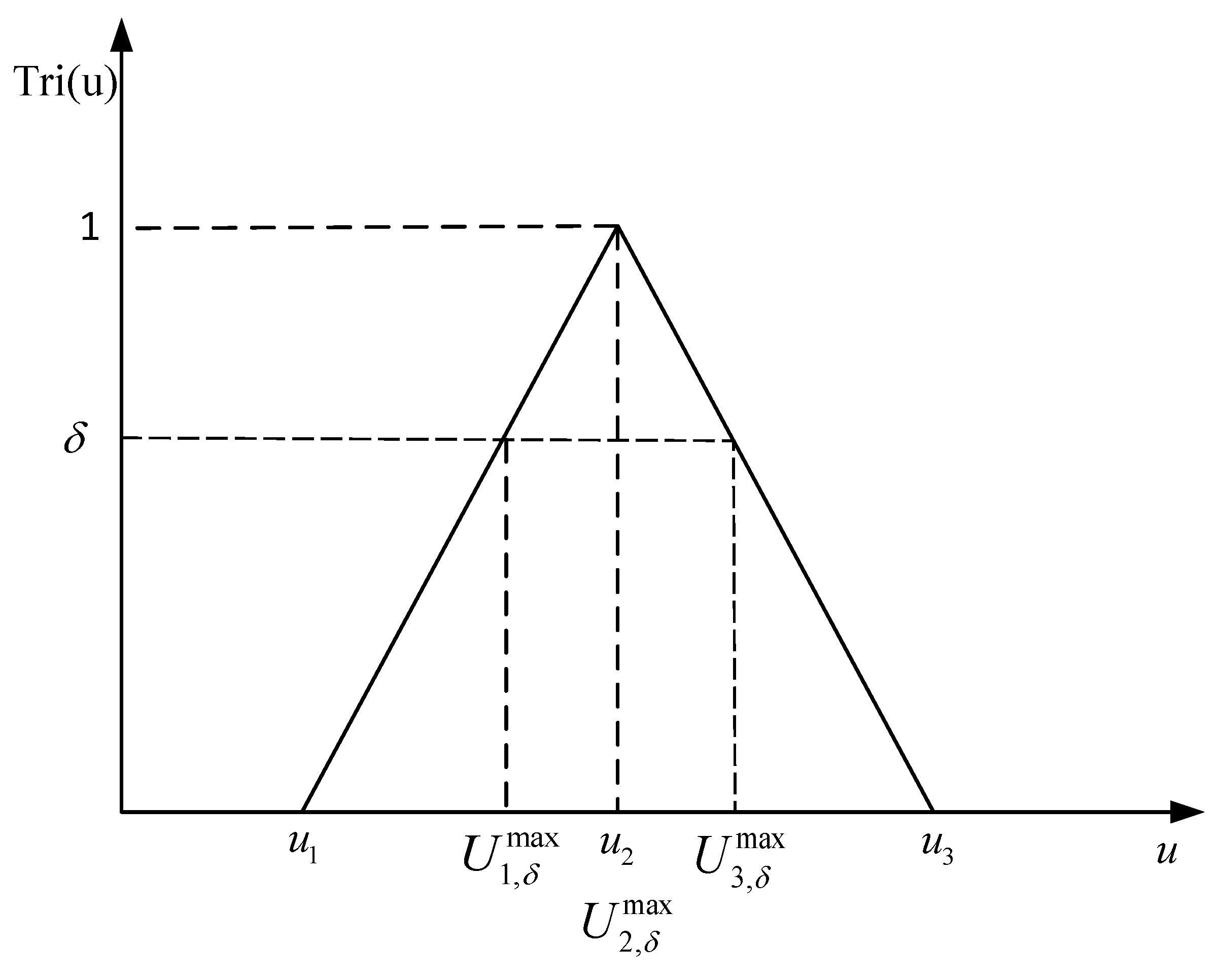
The utility supply ${\widehat{U}}_u^{\max }$ in Constraint (36) is an uncertain parameter. It is assumed that the triangular membership function of ${\widehat{U}}_u^{\max }$ is $T_{ri}(u)$, which is expressed as follows:

$$T_{ri}(u)=\{\begin{array}{c}\frac{u-u_1}{u_2-u_1}{,\mathrm{u}}_1\le u\le u_2;\\ \frac{u_3-u}{u_3-u_2},{\mathrm{u}}_2<u\le u_3;\\ 0,\mathrm{other}.\end{array}$$

(37)

Using the theory of fuzzy knowledge, Constraint (36) can be converted to Constraint (38). Finally, the uncertain model with utility constraints is transformed into a deterministic model with membership degree.

$${\displaystyle \sum _{i\in I_u}({\lambda }_{iu}\cdot w(i,n))}+{\displaystyle \sum _{i\in I_u}({\phi }_{iu}}\cdot b(i,n))\le w_1\cdot U_{1,\delta }^{\max }+w_2\cdot U_{2,\delta }^{\max }+w_3\cdot U_{3,\delta }^{\max };u\in U,n\in N.$$

(38)

$w_1$,$w_2$,$w_3$ are the weights, and $w_1+w_2+w_3=1$; the fuzzy parameters of High-pressure Steam (HS) and Cooling Water (CW) include the most pessimistic value, the most possible value, and the most optimistic value. The three prominent values, i.e., the most pessimistic, the most possible, and the most optimistic values for each fuzzy number are usually estimated by decision maker [37,38]. In this paper, the three prominent values are defined according to determining method of universe and the experience of engineering. The universe $U$ of fuzzy number is defined as an equation according to Basyigit and Ulu [39], where $D_{min}$ is the minimum value in statistical data of fuzzy number, $D_{max}$ is the maximum value in statistical data of fuzzy number. $D_1$ and $D_2$ are defined as an equation and according to the experience of engineering. $D_{mf}$ is the value of which the frequency of occurrence is the highest in statistical data of fuzzy numbers.

$$U=[D_{min}-D_1,D_{ma\mathrm{x}}+D_2],$$

(39)

$$D_1=0.2\ast \left|D_{min}-D_{mf}\right|,$$

(40)

$$D_2=0.2\ast \left|D_{ma\mathrm{x}}-D_{mf}\right|.$$

(41)

In order to describe fuzzy numbers more generally, in this paper we define $u_1$, $u_2$ and $u_3$ as the most pessimistic value, the most possible value, and the most optimistic value. The most pessimistic value $u_1$ is equal to $D_{min}-D_1$ (the left boundary of universe). The most possible value $u_2$ is equal to $D_{mf}$. The most optimistic value $u_3$ is equal to $D_{ma\mathrm{x}}+D_2$ (the right boundary of universe).

$$u_1=D_{min}-D_1,$$

(42)

$$u_2=D_{mf},$$

(43)

$$u_3=D_{max}+D_2.$$

(44)

The triangular membership degrees of $U_{1,\delta }^{\max }$, $U_{2,\delta }^{\max }$, $U_{3,\delta }^{\max }$ are the boundary points of $U_u^{\max }$ under the cut set $\delta$, the corresponding calculation formula of the boundary point is as follows, and the relationship between them is shown in Figure 1.

$$U_{1,\delta }^{\max }=u_1+\delta \cdot (u_2-u_1),$$

(45)

$$U_{2,\delta }^{\max }=u_2,$$

(46)

$$U_{3,\delta }^{\max }=u_3-\delta \cdot (u_3-u_2).$$

(47)

3. Integrated Model and Solving Strategy

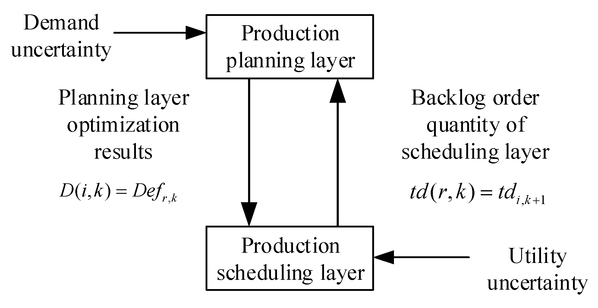
In this paper, the integrated model of production planning and scheduling considering demand uncertainty and utility uncertainty is solved based on the integrated optimization method and rolling horizon optimization strategy. The solving method of integrated optimization is to construct a bi-level integrated model of planning and scheduling to deal with the demand and utility uncertainties. As the uncertainty of demand and utility are different in time scales, it is necessary to deal with the uncertainty of demand and utility in production planning layer and scheduling layer respectively. The discrete-time model is established in the production planning layer, and chance constrained programming is used to describe demand uncertainty. The continuous-time model is established in the production scheduling layer, and fuzzy theory is used to describe utility uncertainty. When the planning layer completes the Kth optimization, the optimization result $D(i,k)$ corresponding to the first planning period is equal to $De{f}_{r,k}$. Parameter $De{f}_{r,k}$ is assigned as a task to the scheduling layer. The double-layer structure of production planning and scheduling is shown in Figure 2.

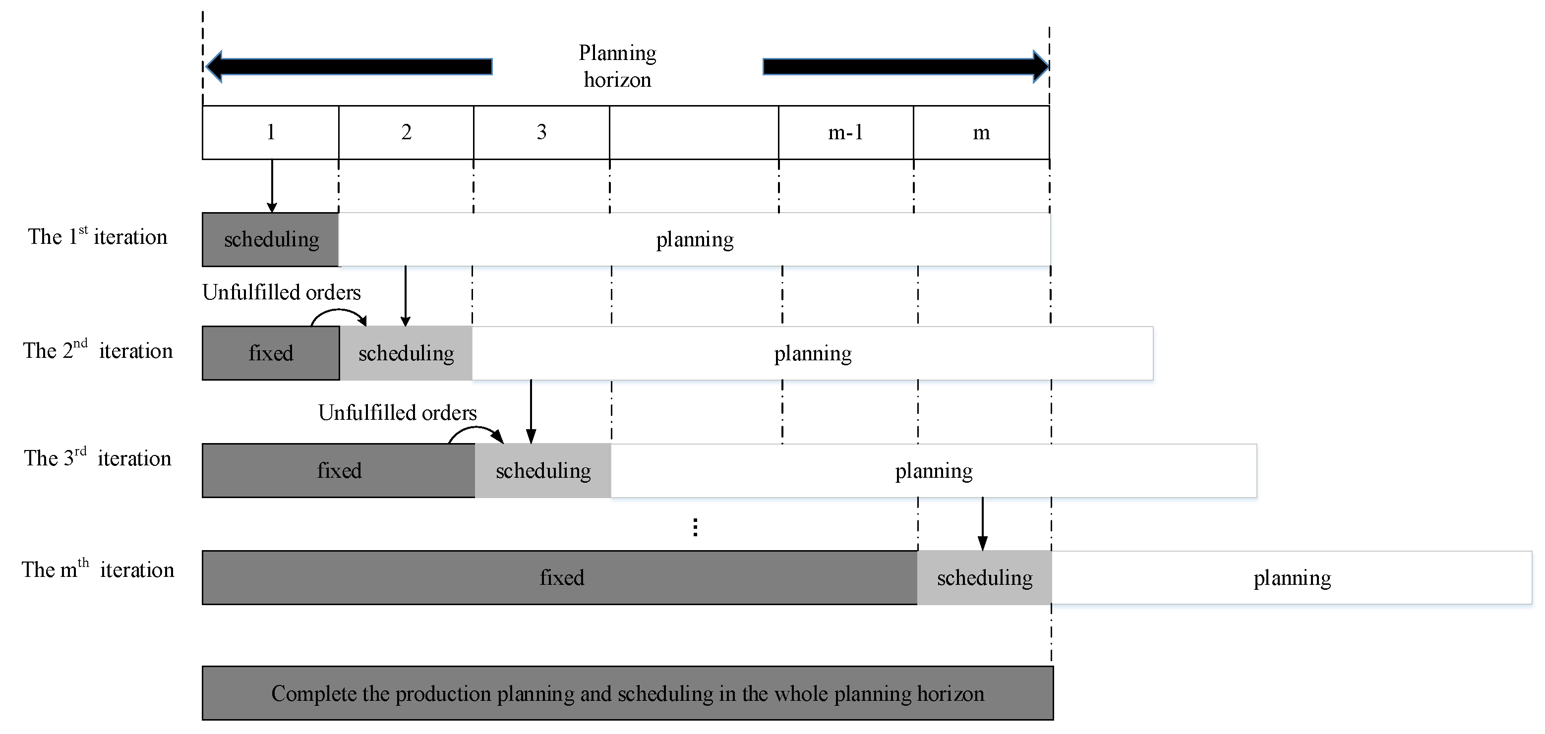
Rolling horizon optimization strategy is a general time decomposition method. The planning horizon of the discrete-time model in the planning layer is composed of $m$ planning periods with equal time durations. The scheduling horizon of the continuous-time model in the scheduling layer is equal to the length of the planning period. The rolling horizon optimization strategy is used to iteratively solve the integrated model of production planning and scheduling. The specific steps of rolling horizon optimization strategy are as follows:

a. Solve the production planning model and assign the delivery quantity of the first planning period to the scheduling model.

b. Solve the scheduling model of the current period and judge whether the scheduling layer has completed the delivery quantity assigned by the planning layer. If it can be completed, roll the planning horizon and repeat step a; if it cannot be completed, the unfinished tasks will be passed to the next planning period as the backlog order quantity, then roll the planning horizon and repeat the step a.

c. The calculation is terminated after obtaining the planning and scheduling schemes for all periods.

The flow chart of iterative solving strategy of integrated model is shown in Figure 3, and the schematic diagram of rolling horizon optimization strategy is shown in Figure 4.

4. Case Study

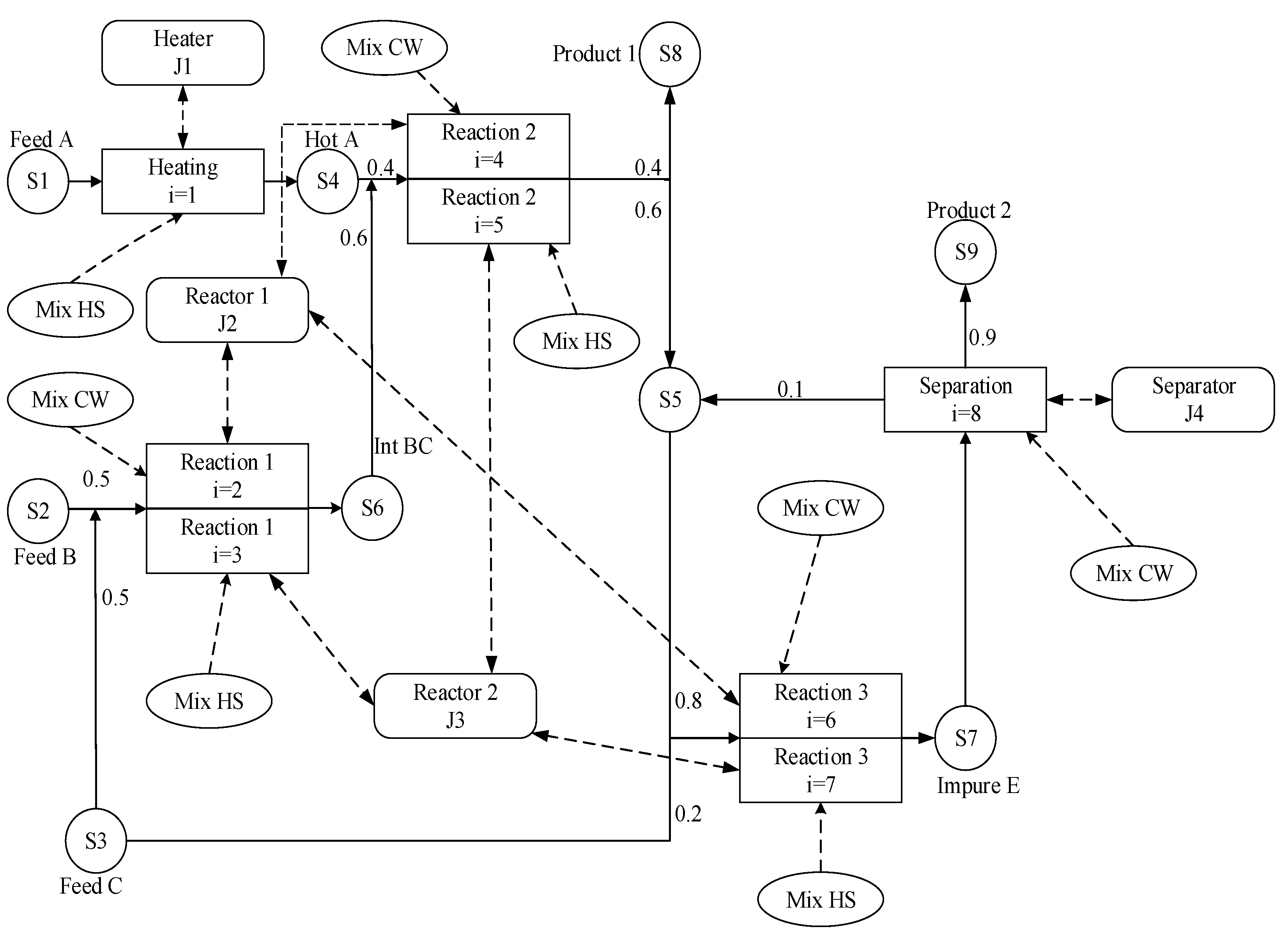
The classical example [40] was used to verify the feasibility and effectiveness of the two-layer integrated model of planning and scheduling in dealing with the uncertain problems of demand and utility based on the RTN representation. The example uses RTN representation to describe the production process, as shown in Figure 5. The three raw materials S1, S2 and S3 produce two products S8 and S9 through a series of endothermic and exothermic reactions, in which the endothermic reaction requires high-pressure steam (HS) and the exothermic reaction requires condensed water (CW). Due to the limitations of the energy system, the average supply of HS and CW is 64 and 69 kg/min, respectively. Heating can be performed on heater J1. Reaction 1 can be performed on reactors J2, J3. Reaction 2 can be performed on reactors J2, J3. Reaction 3 can be performed on reactors J2, J3. Separation can be performed on separator J4. The study involved a total of eight different production processes. Unlimited storage policy is adopted for raw materials and products, and limited storage policy is adopted for intermediate materials [41,42]. The relevant data of the calculation example are shown in

Table 1. Task processing time coefficient and capacity data.

Task (i)	Unit (j)	${\mathit{\alpha }}_{\mathit{i}}$	${\mathit{\beta }}_{\mathit{i}}$	${\mathit{B}}_{\mathit{i}}^{\mathbf{min}}$	${\mathit{B}}_{\mathit{i}}^{\mathbf{max}}$
Heating (i = 1)	Heater	0.667	0.00667	-	100
Reaction 1 (i = 2)	Reactor 1	1.334	0.02664	-	50
Reaction 1 (i = 3)	Reactor 2	1.334	0.01665	-	80
Reaction 2 (i = 4)	Reactor 1	1.334	0.02664	-	50
Reaction 2 (i = 5)	Reactor 2	1.334	0.01665	-	80
Reaction 3 (i = 6)	Reactor 1	0.667	0.01332	-	50
Reaction 3 (i = 7)	Reactor 2	0.667	0.008325	-	80
Separation (i = 8)	Separator	1.3342	0.00666	-	200

,

Table 2. Material and device resource related data.

Resource	Capacity (kg)	Initial (kg)	Price ($/kg)
S1	UL	AA	0
S2	UL	AA	0
S3	UL	AA	0
S4	100	0	0
S5	200	0	0
S6	150	0	0
S7	200	0	0
S8	UL	0	40
S9	UL	0	30
Heater	1	1	-
Reactor1	1	1	-
Reactor2	1	1	-
Separator	1	1	-

UL—Unlimited; AA—available as and when required.

and

Table 3. Utility consumption coefficient.

Task (i)	${\mathit{\lambda }}_{\mathit{i}\mathit{H}\mathit{S}}$ $(\mathit{k}\mathit{g}\cdot {\mathbf{min}}^{-1})$	${\mathit{\phi }}_{\mathit{i}\mathit{H}\mathit{S}}$ $(\mathit{k}\mathit{g}\cdot {\mathbf{min}}^{-1})$	${\mathit{\lambda }}_{\mathit{i}\mathit{C}\mathit{W}}$ $(\mathit{k}\mathit{g}\cdot {\mathbf{min}}^{-1})$	${\mathit{\varphi }}_{\mathit{i}\mathit{C}\mathit{W}}$ $(\mathit{k}\mathit{g}\cdot {\mathbf{min}}^{-1})$
i = 1	6	0.25	-	-
i = 2	-	-	4	0.25
i = 3	5	0.25	-	-
i = 4	-	-	4	0.3
i = 5	4	0.5	-	-
i = 6	-	-	3	0.3
i = 7	4	0.2	-	-
i = 8	-	-	6	0.35

.

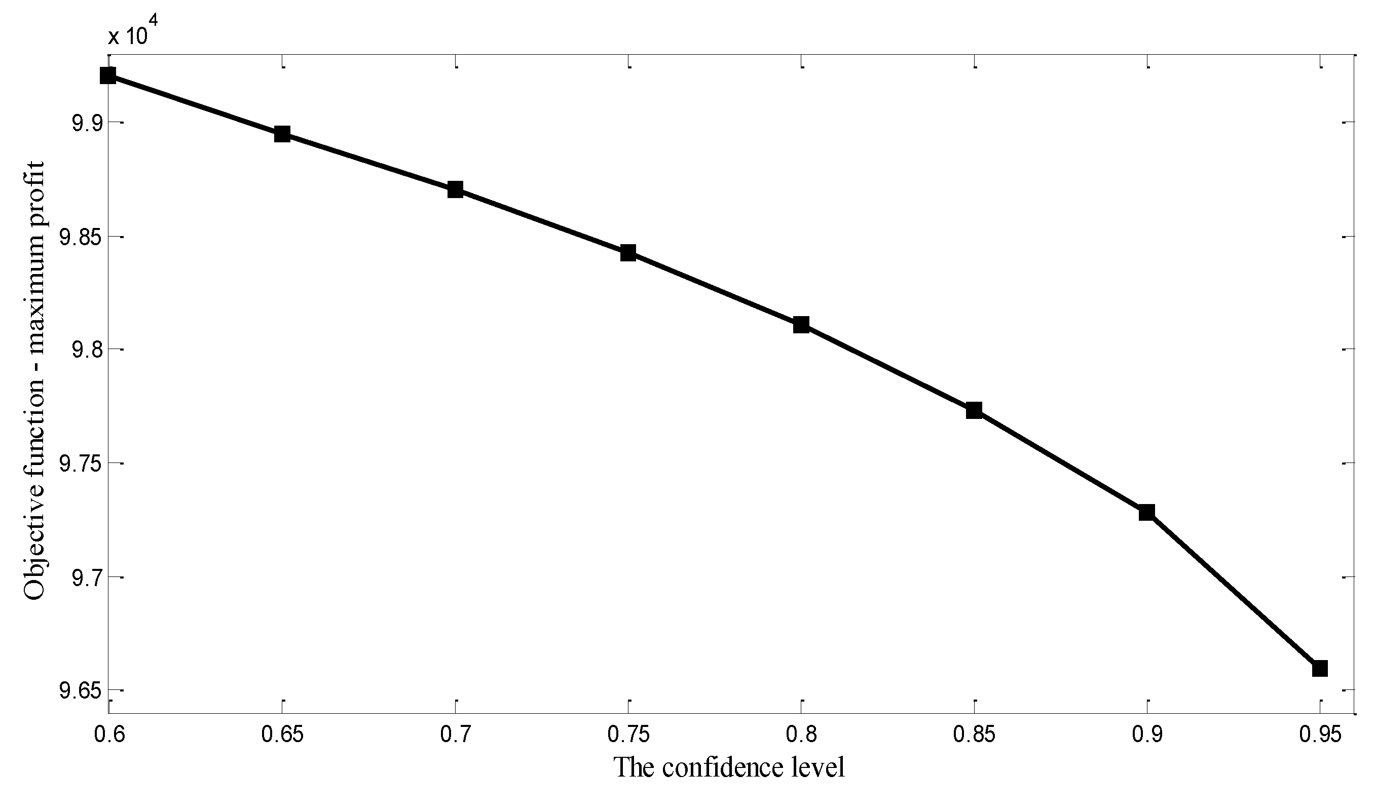
4.1. The Influence of the Planning Layer Confidence Factor on the Optimization Results

The stochastic programming with chance constraints is introduced into the production planning layer to describe the uncertainty of demand. Through a series of mathematical transformation, the uncertain model with chance constraints can be transformed into a deterministic model with specified confidence level. Different confidence levels have a very important impact on the optimization results. The objective functions under different confidence factors are shown in

Table 4. The objective function under different confidence factors.

Confidence Factor	Inverse Function	Objective Function ($)
0.6	−0.25	99,206.36
0.65	−0.39	98,945.22
0.7	−0.52	98,702.73
0.75	−0.67	98,422.94
0.8	−0.84	98,105.84
0.85	−1.04	97,732.78
0.9	−1.28	97,285.11
0.95	−1.65	96,594.95

. The value of the confidence factor in the part of integrated model simulation analysis is 0.9. The variation trend of maximum profit under different confidence levels is shown in Figure 6.

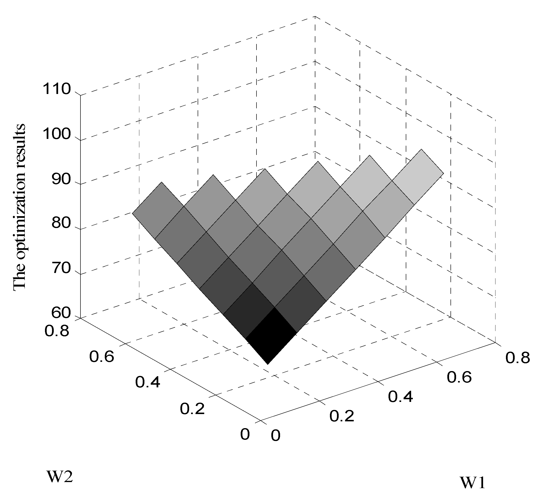
4.2. The Influence of Scheduling Layer Fuzzy Weight on the Optimization Results

In the production scheduling layer, fuzzy theory is introduced to describe the uncertainty of utilities. It is assumed that triangular membership function is adopted to express the uncertainty of utilities. Using the knowledge of fuzzy theory, the uncertainty model with utility is transformed into a certainty model with fuzzy weights. The fuzzy parameter values of HS is $u_1=62,u_2=64,u_3=68;$ and the fuzzy parameter values of CW is $u_1=67,u_2=69,u_3=73$. A visualized sensitivity analysis of fuzzy weights is illustrated in Figure 7. The optimization results of scheduling layer under different weights are shown in

Table 5. Scheduling layer optimization result data under different weights.

${\mathit{w}}_1$	${\mathit{w}}_2$	${\mathit{w}}_3$	Objective Function (kg)
0.1	0.1	0.8	67.59
0.1	0.2	0.7	72.51
0.1	0.3	0.6	77.43
0.1	0.4	0.5	82.35
0.1	0.5	0.4	87.27
0.1	0.6	0.3	92.19
0.1	0.7	0.2	97.11
0.1	0.8	0.1	102.03

. It can be seen from Figure 7 that when the weight of the maximum possible value increases from 0.1 to 0.8, the optimal solution of the uncertain model is closer to the optimal solution of the deterministic model. This is because the weights $w_1$, $w_2$, and $w_3$ represent the degree of inclination of the model to the most optimistic value, the maximum possible value, and the most pessimistic value in the membership function. In other words, if the weight of the boundary is large, the influence of the boundary on the optimization result will be greater. For the fuzzy weights, $w_1$, $w_2$, $w_3$ represent the weights of the most pessimistic, the most possible, and the most optimistic value of the related fuzzy numbers, respectively. In practice, the suitable values for these weights as well as $\delta$ are usually determined subjectively by the experience and knowledge of the decision maker. Based on the most likely value concept proposed by Lai and Hwang [38], and considering several relevant works [43,44], we set these parameters to: $w_1=0.1,w_2=0.5,w_3=0.4$ in this paper.

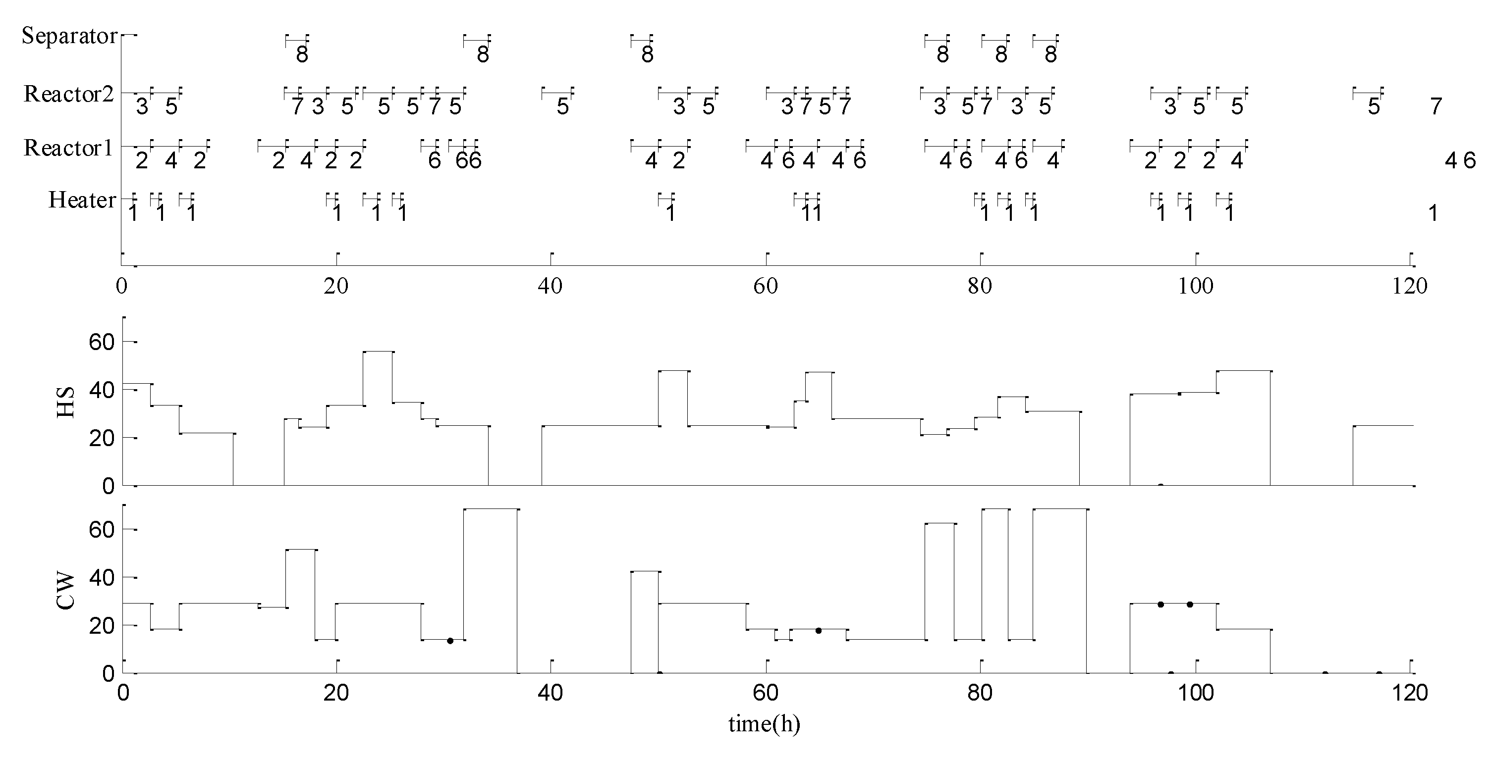
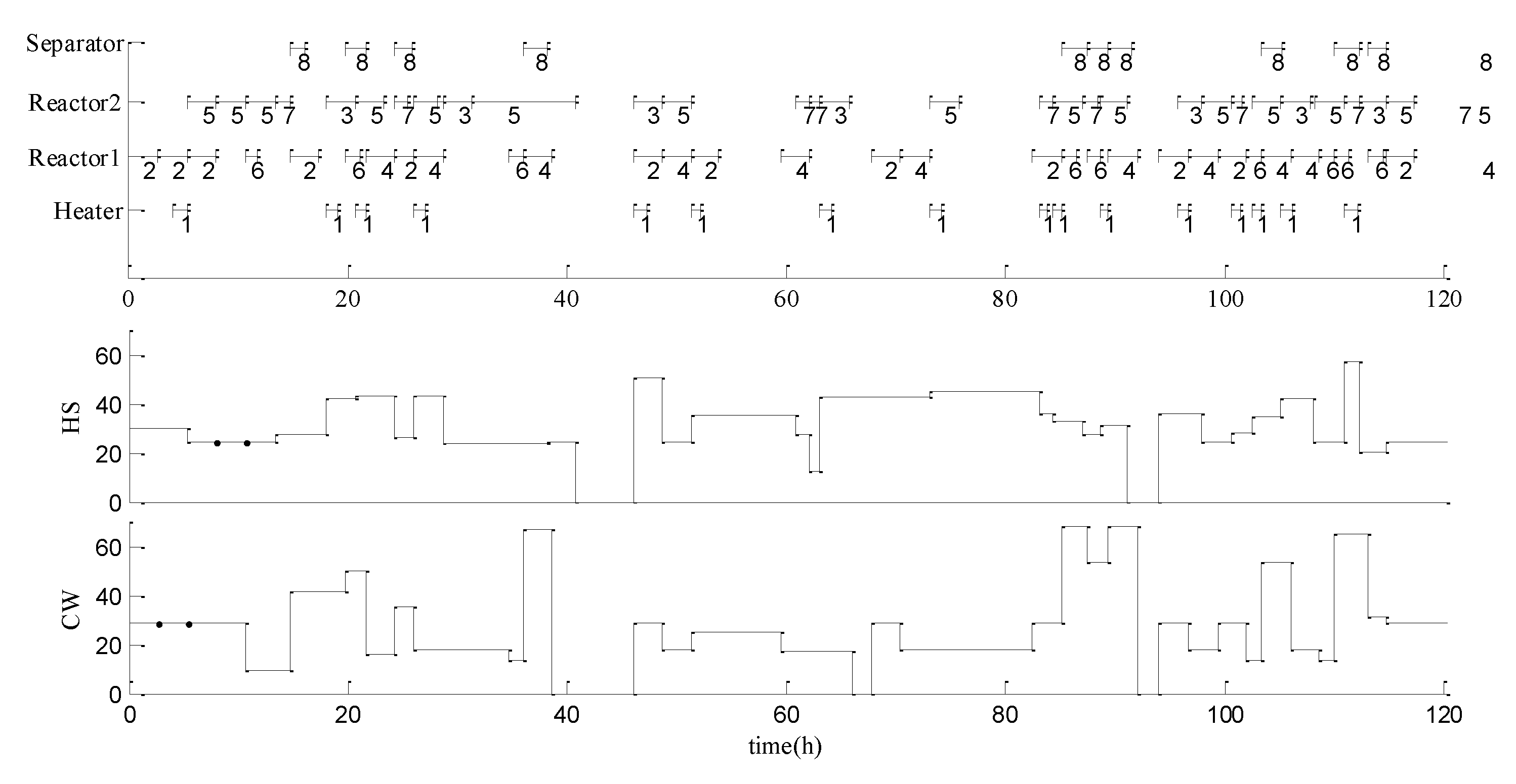
4.3. Integrated Model Simulation Analysis

The order data of two products in nine planning periods and the corresponding average supply of two utilities are given. Based on the RTN representation, integrated optimization solving method and rolling horizon optimization strategy were used to iteratively solve the integrated model to complete the planning and scheduling tasks of the first five planning periods. The software Lingo 11.0 was used for simulation calculation on a 2.20 GHz computer, where the planning horizon is 5 days and the planning period and scheduling horizon are both 1 day. The number of event points is 12. Figure 8 and Figure 9 respectively show the gantt chart and utility consumption level of the deterministic method and the uncertainty method. From Figure 8 and Figure 9, we can intuitively get the respective task number and the corresponding specific utility consumption under the deterministic method and the uncertain method. Under the deterministic method, the solution time of the rolling horizon algorithm is 28 s. Under the uncertain method, the solution time of the rolling horizon algorithm is 34 s.

In the comparative analysis between the deterministic method and the uncertain method shown in

Table 6. Comparative analysis of the planning layer.

Modeling Method	Objective Function ($)	${\mathit{S}}_8^{\mathit{p}\mathit{l}\mathit{a}\mathit{n}}(\mathit{k}\mathit{g})$	${\mathit{S}}_9^{\mathit{p}\mathit{l}\mathit{a}\mathit{n}}(\mathit{k}\mathit{g})$
Deterministic method	99,688.52	1330	1550
Uncertain method	97,285.11	1296.998	1514.416

and

Table 7. Comparative analysis of the scheduling layer.

Modeling Method	Objective Function ($)	${\mathit{S}}_8^{\mathit{p}\mathit{l}\mathit{a}\mathit{n}}(\mathit{k}\mathit{g})$	${\mathit{S}}_9^{\mathit{p}\mathit{l}\mathit{a}\mathit{n}}(\mathit{k}\mathit{g})$
Deterministic method	128.9	1201.1	1550
Uncertain method	87.277	1209.721	1514.416

, $S_8^{plan}$ and $S_9^{plan}$ respectively represent the planned production of $S_8$ and $S_9$; $S_8^{schedule}$ and $S_9^{schedule}$ represent the scheduled production of $S_8$ and $S_9$ respectively. The objective function of the planning layer of the deterministic method is $99,688.52, and the output of products $S_8$ and $S_9$ in the planning layer are, respectively, 1330 and 1550 kg. In the uncertain method with the confidence factor of 0.9, the objective function of the planning layer is $97,285.11, and the output of products $S_8$ and $S_9$ are respectively 1296.998 and 1514.416 kg. The objective function in the scheduling layer of the deterministic method is 128.9 kg, and the output of products $S_8$ and $S_9$ are, respectively, 1201.1 and 1550 kg. The objective function in the scheduling layer of the uncertain method is 87.277 kg, and the output of products $S_8$ and $S_9$ are, respectively, 1209.721 and 1514.416 kg. The final profit of the enterprise under the deterministic method is $86,792.96, and the final profit of the enterprise under the uncertain method is $88,557.392. The comparison of the final profit shows that the uncertain method reflects the actual production process more realistically due to considering the uncertainty of the demand and the utility, which brings greater profits to the enterprise.

Table 8. The consumption amount of each period of utility under the deterministic method.

$\mathit{u}\mathit{t}\mathit{i}\mathit{l}\mathit{i}\mathit{t}\mathit{y}$	$\mathit{u}\mathit{s}{\mathit{e}}_1(\mathit{k}\mathit{g})$	$\mathit{u}\mathit{s}{\mathit{e}}_2(\mathit{k}\mathit{g})$	$\mathit{u}\mathit{s}{\mathit{e}}_3(\mathit{k}\mathit{g})$	$\mathit{u}\mathit{s}{\mathit{e}}_4(\mathit{k}\mathit{g})$	$\mathit{u}\mathit{s}{\mathit{e}}_5(\mathit{k}\mathit{g})$	$\mathit{u}\mathit{s}{\mathit{e}}_{\mathit{a}\mathit{l}\mathit{l}}(\mathit{k}\mathit{g})$
HS	352.31419	345.83433	383.03704	370.31418	353.44445	1804.94419
CW	337.26051	339.90991	357.33333	322.22298	328.33334	1685.06007

and

Table 9. The consumption amount of each period of utility under the uncertain method.

$\mathit{u}\mathit{t}\mathit{i}\mathit{l}\mathit{i}\mathit{t}\mathit{y}$	$\mathit{u}\mathit{s}{\mathit{e}}_1(\mathit{k}\mathit{g})$	$\mathit{u}\mathit{s}{\mathit{e}}_2(\mathit{k}\mathit{g})$	$\mathit{u}\mathit{s}{\mathit{e}}_3(\mathit{k}\mathit{g})$	$\mathit{u}\mathit{s}{\mathit{e}}_4(\mathit{k}\mathit{g})$	$\mathit{u}\mathit{s}{\mathit{e}}_5(\mathit{k}\mathit{g})$	$\mathit{u}\mathit{s}{\mathit{e}}_{\mathit{a}\mathit{l}\mathit{l}}(\mathit{k}\mathit{g})$
HS	339.07849	371.35303	340.01582	343.52171	341.69782	1735.66687
CW	340.84803	359.11669	372.16621	330.04896	330.19241	1732.3723

respectively represent the consumption amount of utility in each period under the deterministic method and uncertain method, where $us{e}_i(i=1\cdots 5)$ represents the consumption amount of utility in the planning period $i$ and $us{e}_{all}$ represents the total usage amount of utility. The total amounts of utility HS used under the deterministic method and the uncertain method are 1804.94419 and 1735.6687 kg, respectively. The total amounts of utility CW used under the deterministic method and the uncertain method are 1685.06007 and 1732.3723 kg, respectively.

Backlog order quantity of 87.277 kg under the uncertain method is significantly less than that of 128.9 kg under the deterministic method. These comparative results show that introducing the uncertain programming method into the planning and scheduling layers, respectively, can greatly reduce the generation of backlog order quantity, and the scheduling layer can more effectively complete the tasks assigned by the planning layer. Based on the RTN representation, the uncertain method adopted in the scheduling layer can effectively reduce the impact of uncertainty factors on the optimization results, and can clearly count the consumption amount of utilities in each period. Therefore, the proposed integrated model can more realistically reflect the actual production situation, save energy, and reduce production costs, so that the final profit of the enterprise obtained by the uncertain method is $88,557.392, which is obviously better than the final profit of the enterprise under the deterministic method of $86,792.96.

Considering the uncertainty of demand and utility, the proposed method is slightly more complex than the deterministic model in modeling and solving, but it belongs to the category of pre-scheduling, and the solving time is 34 s, which can fully meet the real-time requirements of actual production. In addition, this method has more application value for chemical enterprises whose demand is affected by seasons and which need utilities, especially for small businesses. In order to reduce the cost, small businesses will be gathered and purchase utilities from other companies to support their own production. Compared with large enterprises which have their own energy systems, the utilities supply for small businesses experiences disturbance more easily. Consequently, for this kind of small business, considering the uncertain utility problem for effective enterprise production process is of great application value and practical significance.

5. Conclusions

This paper introduces and analyzes uncertain factors involved in production planning and scheduling. According to the property of time scale, these uncertain factors are dealt with distinctively in the planning and scheduling layers. The planning layer and scheduling layer models are formulated by discrete-time and continuous-time modeling methods, respectively. Chance constrained programming and fuzzy theory are introduced into planning layer model and scheduling layer model, respectively, to describe the uncertainties of demand and utility. Rolling horizon optimization strategy is utilized to solve the bi-level integrated model iteratively. Through comparison, simulation results show that the proposed model and algorithm are feasible and effective, can calculate the consumption of utility in every period, decrease the effects of uncertain factors on optimization results, and more accurately reflect the actual production process.

References

- Chu, Y.; You, F.; Wassick, J.M.; Agarwal, A. Integrated planning and scheduling under production uncertainties: Bi-level model formulation and hybrid solution method. Comput. Chem. Eng. 2015, 72, 255–272. [Google Scholar] [CrossRef]
- An, Y.W.; Yan, H.S. Solution Strategy of Integrated Optimization of Production Planning and Scheduling in a Flexible Job-shop. Acta Autom. Sin. 2013, 39, 1476–1491. [Google Scholar] [CrossRef]
- Li, W.; Ong, S.K.; Nee, A.Y.C. A Unified Model-based Integration of Process Planning and Scheduling. In Process Planning & Scheduling for Distributed Manufacturing; Springer: London, UK, 2007; pp. 295–309. [Google Scholar]
- Shao, X.; Li, X.; Liang, G.; Zhang, C. Integration of process planning and scheduling—A modified genetic algorithm-based approach. Comput. Oper. Res. 2009, 36, 2082–2096. [Google Scholar] [CrossRef]
- Lasserre, J.B. An Integrated Model for Job-Shop Planning and Scheduling. Manag. Sci. 1992, 38, 1201–1211. [Google Scholar] [CrossRef]
- Xiong, F.; Yan, H.S. Integrated production planning and scheduling of multi-stage workshop based on alternant iterative genetic algorithm. J. Southeast Univ. (Nat. Sci. Ed.) 2012, 42, 183–187. [Google Scholar]
- Li, Z.K.; Ierapetritou, M.G. Production planning and scheduling integration through augmented Lagrangian optimization. Comput. Chem. Eng. 2010, 34, 996–1006. [Google Scholar] [CrossRef]
- Wang, Y.; Su, H.Y.; Shao, H.S.; Lu, S.; Xie, L. Integration of Production Planning and Scheduling under Demand and Utility Uncertainties. J. Zhejiang Univ. (Eng. Sci.) 2017, 51, 57–67. [Google Scholar]
- Vogel, T.; Almada-Lobo, B.; Almeder, C. Integrated versus hierarchical approach to aggregate production planning and master production scheduling. OR Spectr. 2017, 39, 193–229. [Google Scholar] [CrossRef]
- Hassani, Z.I.M.; El Barkany, A.; Jabri, A.; El Abbassi, I.; Darcherif, A.M. New Approach to Integrate Planning and Scheduling of Production System: Heuristic Resolution. Int. J. Eng. Res. Afr. 2018, 39, 156–169. [Google Scholar] [CrossRef]
- Pantelides, C.C. Unified Frameworks for the Optimal Process Planning and Scheduling. In Proceedings of the Second Conference on the Foundations of Computer Aided Process Operations, Crested Butte, CO, USA, 18–23 July 1993; CACHE Publications: New York, NY, USA, 1994; pp. 253–274. [Google Scholar]
- Zhang, X.; Sargent, R.W.H. The optimal operation of mixed production facilities—A general formulation and some approaches for the solution. Comput. Chem. Eng. 1996, 20, 897–904. [Google Scholar] [CrossRef]
- Castro, P.; Barbosa-Póvoa, A.P.F.D.; Matos, H. An Improved RTN Continuous-Time Formulation for the Short-term Scheduling of Multipurpose Batch Plants. Ind. Eng. Chem. Res. 2001, 40, 2059–2068. [Google Scholar] [CrossRef]
- Chen, G. Modeling and Optimization for Short-term Scheduling of Multipurpose Batch Plants. Chin. J. Chem. Eng. 2014, 22, 682–689. [Google Scholar] [CrossRef]
- Schilling, G.; Pantelides, C.C. A simple continuous-time process scheduling formulation and a novel solution algorithm. Comput. Chem. Eng. 1996, 20, S1221–S1226. [Google Scholar] [CrossRef]
- Dimitriadis, A.D.; Shah, N.; Pantelides, C.C. RTN-based rolling horizon algorithms for medium term scheduling of multipurpose plants. Comput. Chem. Eng. 1997, 21, S1061–S1066. [Google Scholar] [CrossRef]
- Chao, S.; You, F. Distributionally robust optimization for planning and scheduling under uncertainty. Comput. Chem. Eng. 2017, 110, 53–68. [Google Scholar]
- Curcio, E.; Amorim, P.; Qi, Z.; Almada-Lobo, B. Adaptation and approximate strategies for solving the lot-sizing and scheduling problem under multistage demand uncertainty. Int. J. Prod. Econ. 2018, 202, 81–96. [Google Scholar] [CrossRef]
- Li, P.; Wendt, M.; Wozny, G. Optimal production planning under uncertain market conditions. Comput. Aided Chem. Eng. 2003, 15, 511–516. [Google Scholar]
- Wang, Y.; Jin, X.; Xie, L.; Zhang, Y.; Lu, S. Uncertain Production Scheduling Based on Fuzzy Theory Considering Utility and Production Rate. Information 2017, 8, 158. [Google Scholar] [CrossRef]
- Chen, Q.X.; Jiao, B.; Yan, S.B. Flow Shop Production Scheduling under Uncertainty within Infinite Intermediate Storage. Adv. Mater. Res. 2011, 204–210, 777–783. [Google Scholar] [CrossRef]
- Lamba, N.; Karimi, I.A. Scheduling Parallel Production Lines with Resource Constraints. 1. Model Formulation. Ind. Eng. Chem. Res. 2002, 41, 790–800. [Google Scholar] [CrossRef]
- Méndez, C.A.; Cerdá, J. An MILP framework for short-term scheduling of single-stage batch plants with limited discrete resources. Comput. Aided Chem. Eng. 2002, 10, 721–726. [Google Scholar]
- Tian, Y. Chemical Production Planning and Scheduling Integration under Uncertainty. J. Chem. Ind. 2014, 65, 3552–3558. [Google Scholar]
- Chand, S.; Traub, R.; Uzsoy, R. Rolling horizon procedures for the single machine deterministic total completion time scheduling problem with release dates. Ann. Oper. Res. 1997, 70, 115–125. [Google Scholar] [CrossRef]
- Bonfill, A.; Bagajewicz, M.; Espuña, A.; Puigjaner, L. Risk management in the scheduling of batch plants under uncertain market demand. Ind. Eng. Chem. Res. 2004, 43, 741–750. [Google Scholar] [CrossRef]
- Chanas, S.; Kasperski, A. Minimizing maximum lateness in a single machine scheduling problem with fuzzy processing times and fuzzy due dates. Eng. Appl. Artif. Intell. 2001, 14, 377–386. [Google Scholar] [CrossRef]
- Ning, C.; You, F. A data-driven multistage adaptive robust optimization framework for planning and scheduling under uncertainty. AIChE J. 2017, 63, 4343–4369. [Google Scholar] [CrossRef]
- Leung, S.C.H.; Tsang, S.O.S.; Ng, W.L.; Wu, Y. A robust optimization model for multi-site production planning problem in an uncertain environment. Eur. J. Oper. Res. 2007, 181, 224–238. [Google Scholar] [CrossRef]
- Iris, Ç.; Lam, J.S.L. Recoverable robustness in weekly berth and quay crane planning. Transp. Res. Part B Methodol. 2019, 122, 365–389. [Google Scholar] [CrossRef]
- Cheng, H.N.; Xiang, S.G.; Yang, X.; Han, F.Y. Supply chain planning model under uncertainty. Comput. Appl. Chem. 2004, 21, 97–102. [Google Scholar]
- Safaei, A.S.; Farsad, S.; Paydar, M.M. Emergency logistics planning under supply risk and demand uncertainty. Oper. Res. 2018. Available online: https://doi.org/10.1007/s12351-018-0376-3 (accessed on 30 January 2018).
- Englberger, J.; Herrmann, F.; Manitz, M. Two-stage stochastic master production scheduling under demand uncertainty in a rolling planning environment. Int. J. Prod. Res. 2016, 54, 6192–6215. [Google Scholar] [CrossRef]
- Fajie Wei, R.Z. Activity-Oriented Production Theory and Cost Theory of Enterprises; Beijing University of Aeronautics and Astronautics Press: Beijing, China, 2007. [Google Scholar]
- Wang, Y. Research on Production Planning and Scheduling under Uncertainty. Ph.D. Thesis, Zhejiang University, Hangzhou, China, 2016. [Google Scholar]
- Iris, C.; Cevikcan, E. A fuzzy linear programming approach for aggregate production planning. In Supply Chain Management under Fuzziness; Springer: Berlin/Heidelberg, Germany, 2014; pp. 355–374. [Google Scholar]
- Torabi, S.A.; Ebadian, M.; Tanha, R. Fuzzy hierarchical production planning (with a case study). Fuzzy Sets Syst. 2010, 161, 1511–1529. [Google Scholar] [CrossRef]
- Lai, Y.J.; Hwang, C.L. A new approach to some possibilistic linear programming problems. Fuzzy Sets Syst. 1992, 49, 121–133. [Google Scholar] [CrossRef]
- Basyigit, A.; Ulu, C.; Guzelkaya, M. A New Fuzzy Time Series Model Using Triangular and Trapezoidal Membership Functions. In Proceedings of the International Work-Conference on Time Series, Granada, Spain, 25–27 June 2014; pp. 25–27. [Google Scholar]
- Li, Z.; Ierapetritou, M.G. Rolling horizon based planning and scheduling integration with production capacity consideration. Chem. Eng. Sci. 2010, 65, 5887–5900. [Google Scholar] [CrossRef]
- And, M.G.I.; Floudas, C.A. Effective Continuous-Time Formulation for Short-Term Scheduling. 1. Multipurpose Batch Processes. Ind. Eng. Chem. Res. 1998, 37, 4341–4359. [Google Scholar]
- Mokhtari, H.; Abadi, I.N.K.; Zegordi, S.H. Production capacity planning and scheduling in a no-wait environment with controllable processing times: An integrated modeling approach. Expert Syst. Appl. 2011, 38, 12630–12642. [Google Scholar] [CrossRef]
- Garciasabater, J.P. Capacity and material requirement planning modelling by comparing deterministic and fuzzy models. Int. J. Prod. Res. 2008, 46, 5589–5606. [Google Scholar] [Green Version]
- Christou, I.; Lagodimos, A.; Lycopoulou, D. Hierarchical production planning for multi-product lines in the beverage industry. Prod. Plan. Control 2007, 18, 367–376. [Google Scholar] [CrossRef]
Figure 1.
The triangular membership function of parameter .
Figure 2.
The double-layer structure of production planning and scheduling.
Figure 3.
Flow chart of integrated model iterative solving strategy.
Figure 4.
Rolling horizon optimization strategy.
Figure 5.
Resource-Task Network diagram.
Figure 6.
The variation trend of maximum profit under different confidence levels.
Figure 7.
Scheduling layer optimization results under different weights.
Figure 8.
Gantt chart and utility consumption of the deterministic method.
Figure 9.
Gantt chart and utility consumption of the uncertain method.