An Improved Squirrel Search Algorithm for Global Function Optimization


School of Electrical Engineering, Northeast Electric Power University, Jilin 132012, China
*
Author to whom correspondence should be addressed.
Algorithms 2019, 12(4), 80; https://doi.org/10.3390/a12040080
Submission received: 10 March 2019
/
Revised: 11 April 2019
/
Accepted: 12 April 2019
/
Published: 17 April 2019
Abstract
:An improved squirrel search algorithm (ISSA) is proposed in this paper. The proposed algorithm contains two searching methods, one is the jumping search method, and the other is the progressive search method. The practical method used in the evolutionary process is selected automatically through the linear regression selection strategy, which enhances the robustness of squirrel search algorithm (SSA). For the jumping search method, the ‘escape’ operation develops the search space sufficiently and the ‘death’ operation further explores the developed space, which balances the development and exploration ability of SSA. Concerning the progressive search method, the mutation operation fully preserves the current evolutionary information and pays more attention to maintain the population diversity. Twenty-one benchmark functions are selected to test the performance of ISSA. The experimental results show that the proposed algorithm can improve the convergence accuracy, accelerate the convergence speed as well as maintain the population diversity. The statistical test proves that ISSA has significant advantages compared with SSA. Furthermore, compared with five other intelligence evolutionary algorithms, the experimental results and statistical tests also show that ISSA has obvious advantages on convergence accuracy, convergence speed and robustness.
1. Introduction
Optimization is one of the most common problems in the engineering field, and with the development of new technology, the problems that need to be optimized have gradually turn to large scale, multi peak and nonlinear approaches. The intelligence evolutionary algorithm is a mature global optimization method with high robustness and wide applicability. The fact that the evolutionary process is not constrained by search space and does not require other auxiliary information means that the intelligence evolutionary algorithm can deal with complex problems effectively, which are too difficult to be solved by the traditional optimization algorithms [1,2]. The applications of the intelligence evolutionary algorithms have covered system control, machine design and engineering planning, for example [3,4,5,6,7].
The intelligence evolutionary algorithms can be divided into the evolutionary heuristic algorithms, the physical heuristic algorithms and the group heuristic algorithms, according to their inspiration. The evolutionary heuristic algorithms originate from the genetic evolution process, with the representative algorithms described as follows: The genetic algorithm imitates Darwin’s theory of natural selection and finds the optimal solution by selection, crossover and mutation [8]. Similarly, the essence of the differential evolutionary algorithm is the genetic algorithm based on real coding; the mutation operation modifies each individual according to the difference vectors of population [9]. In the covariance-matrix adaptation evolution strategy, the direction of mutation steps of a population is directly described by the covariance matrix, where the search range of the next generation is increased or decreased adaptively. The individuals produced by sampling are optimized through the iterative loop [10]. The clonal selection algorithm is based on the clonal selection theory; the fitness value corresponds to the cell affinity, and the optimization process imitates the affinity maturation process of cells with low antigen affinity [11]. Given that human beings have higher survivability because they are good at observing and drawing experience from others’ habits, the social cognitive optimization algorithm was proposed, with better solutions being selected by the imitating process and new solutions being produced by the observing process [12]. Imitating the toning process of musicians, the melody search is aimed at finding the best melody of continuity, the harmony memory considering rate controls the search range of each solution (harmony) and the pitch adjusting rate produces a local perturbation of the new solution [13]. The teaching-learning-based optimization algorithm is proposed through imitating the teachers’ teaching and the students’ learning process. The teacher is the individual with the best grade (fitness value) and the other individuals in the population are students. In order to improve the grades of the whole class, each student studies from the teacher in the teaching stage and the students learn from each other in learning stage [14]. There are three relationships among living things: mutualism, commensalism and parasitism; creatures can benefit themselves by any of these relationships. The symbiotic organisms search was proposed according to this phenomenon. Each individual interacts with other individuals during the optimization and the better individuals are retained after each interaction [15]. The mouth brooding fish algorithm simulates the symbiotic interaction strategies adopted by organisms to survive and propagate in the ecosystem. The proposed algorithm uses the movement, dispersion and protection behavior of a mouth brooding fish as an update mode, and the individuals in the algorithm are updated after these three stages to find the best possible answer [16].
The physical heuristic algorithms are inspired by physical phenomena, with the representative algorithms as follows: The freedom of molecules increases after a solid melts, and the temperature needs to drop slowly to return to stable solids with minimum energy. Simulated annealing takes the fitness value as the energy of the solid, with the energy decreasing gradually with the optimization proceeding and the optimal solution being found [17]. The gravitational search algorithm is based on the law of universal gravitation—for each individual the fitness value represents its resultant force produced by all the individuals in the population [18]. The magnetic optimization algorithm is inspired by the theory of magnetic field, where the resultant forces of individuals are changed by the field strength and the distance among individuals. The acceleration, the velocity and positions of individuals are also updated, with the individuals reaching the optimum values gradually [19]. Considering the refraction that occurs when light travels from a light scattering medium to a denser medium, the ray optimization algorithm was proposed. For each individual, the normal vector is determined by its optimal solution and the global optimal solution; the optimal solution can be found with the exit rays close to normal [20]. The kinetic energy of gas molecules takes the energy of gas as the fitness value. When the pressure remains unchangeable and the temperature decreases, the molecules gradually accumulate to the position where the temperature is the lowest and the kinetic energy is the smallest in the container [21]. Inspired by the physical phenomenon of water evaporation, the water evaporation optimization algorithm was proposed. The factors that affect the water evaporation rate are taken as the fitness values. According to the water evaporation rate model, the evaporation probability matrix was considered as the individual renewal probability. Considering that the aggregated forms of water molecules are different, the algorithm is divided into a monolayer evaporation phase in the early evolutionary stage and a droplet evaporation phase in the later evolutionary stage [22]. The lightning attachment procedure optimization algorithm simulates the lightning formation process, which takes the test points between cloud and ground as individuals and the corresponding electrical fields represent fitness values. The three evolutionary operations—downward pilot, upward pilot and branch fading—imitate the downward leader movement, the upward leader propagation and the discharge of lightning, respectively [23].
The group heuristic algorithms mainly simulate biological habits in nature. The representative algorithms are as follows: The ant colony optimization algorithm was proposed according to the way that ants leave pheromones on their path during movement, with better paths having more pheromones, and thus better paths have greater possibilities to be chosen by ants. As a result, more and more pheromones will be left on those paths, and the optimal solution will be found with the increasing concentration of pheromones [24]. The particle swarm optimization algorithm is inspired by the behavior of birds seeking food. For each individual, the position is updated by its current speed, its optimal position and the global best position [25]. The artificial bee colony algorithm was proposed by imitating honeybee foraging behavior. The whole population is divided into three groups: the leading bees, the following bees and the detecting bees. The leading bees are responsible for producing a new honey source, while the following bees search greedily near better honey sources. If the quality of the honey source remains unchanged after many iterations, the leading bees will change to detecting bees and continue to search for a high quality honey source [26]. The social spider optimization regards the whole search space as the spiders’ attached web, with the spiders’ positions as the possible solutions of the optimization problem, and the corresponding weights representing the fitness values of individuals. Female and male subpopulations produce offspring through their respective cooperation and mating behavior [27]. The selfish herd theory proves that when animals encounter predators, each individual increases its survival possibilities by aggregating with other individuals in the herd, whether this approach affects the survival probability of other individuals or not. According to this theory, the selfish herd optimizer was proposed, wherein each individual updates the location in this way to obtain a greater probability of survival [28]. Inspired by the foraging process of hummingbirds, the hummingbirds optimization algorithm was proposed. The hummingbird can search according to its cognitive behavior without interacting with other individuals in a self-searching phase. In addition to searching through experience, hummingbirds can also search by using various dominant individuals as guidance information in a guided-search phase, with the two phases cooperating to promote the population evolution [29].
A large number of experimental results show that the intelligence optimization algorithms can obtain, exact or approximate an optimal solution to large-scale optimization problems in a limited time frame. However, there are also disadvantages, such as the convergence speed being not fast enough and easily falling into the local optimal. Therefore, scholars have put forward various new intelligence evolutionary algorithms.
In 2018, the squirrel search algorithm (SSA) [30] was proposed by Jain M. The algorithm imitates the dynamic jumping strategies and the gliding characters of flying squirrels. The mathematical model mainly consists of the location of a food source and the appearance of predators. The whole optimization process includes the summer phase and the winter phase. However, similar to other intelligent evolutionary algorithms, SSA also has some shortcomings, such as low convergence accuracy and slow convergence speed [31,32]. According to SSA, the single winter search method of the global search ability is not enough, which makes the algorithm easily fall into local optimal. Furthermore, the random summer search method decreases the convergence speed, and the convergence precision is also reduced. In order to improve the convergence precision and the convergence speed, this paper proposed an improved squirrel search algorithm (ISSA). The proposed algorithm includes the jumping search method and the progressive search method. When the squirrels meet with predators, the ‘escape’ and ‘death’ operations are introduced into the jumping search method and the ‘mutation’ operation is introduced into the progressive search method. ISSA also chooses the suitable search method through the linear regression selection strategy during the optimization process. Twenty-one benchmark functions are used to evaluate the performance of the proposed algorithm. The experiments contain three parts: the influence of the parameter on ISSA, the comparison of the proposed methods and SSA and the comparison of ISSA and five other improved evolutionary algorithms.
2. The Squirrel Search Algorithm
The standard SSA updates the positions of individuals according to the current season, the type of individuals and whether predators appear [30].
2.1. Initialize the Population
Assuming that the number of the population is N, the upper and lower bounds of the search space are FSU and FSL. N individuals are randomly produced according to Formula (1):
FSi represents the i-th individual, (i = 1…N); rand is a random number between 0 and 1; D is the dimension of the problem.
2.2. Classify the Population
Taking the minimization problem as an example, SSA requires that there is only one squirrel at each tree, assuming the total number of the squirrels is N, therefore, there are N trees in the forest. All the N trees contain one hickory tree and Nfs (1 < Nfs < N) acorn trees; the others are normal trees which have no food. The hickory tree is the best food resource for the squirrels and the acorn tree takes second place. Nfs can be different depending on the different problems. Ranking the fitness values of the population in ascending order, the squirrels are divided into three types: individuals located at hickory trees (Fh), individuals located at acorn trees (Fa) and individuals located at normal trees (Fn). Fh refers to the individual with the minimum fitness value, Fa contains the individuals whose fitness rank 2 to Nfs + 1 and the remaining individuals are noted as Fn. In order to find the better food resource, the destination of Fa is Fh; the destinations of Fn are randomly determined as either Fa or Fh.
2.3. Update the Position
The individuals update their positions by gliding to the hickory trees or acorn trees. The specific updating formulas are shown as Formulas (2) and (3), respectively:
r is a random number between 0 and 1; valued at 0.1 represents the predator appearance probability; if , then no predator appears, the squirrels glide in the forest to find the food, and the individuals are safe; if , the predators appear, the squirrels are forced to narrow the scope of activities, the individuals are endangered, and their positions are relocated randomly (the specific method will be introduced in Section 2.4); t represents the current iteration; Gc is the constant with the value of 1.9; Fai (i = 1,2,…Nfs) is the individual randomly selected from Fa; dg is the gliding distance which can be calculated by Formula (4):
hg is the constant valued 8; sf is the constant valued 18; represents the gliding angle which can be calculated by Formula (5):
D is the drag force and L is the lift force which can be calculated by calculated by Formulas (6) and (7), respectively:
, V, S and CD are all the constants which are equal to 1.204 kg m−3, 5.25 ms−1, 154 cm2 and 0.6, respectively; CL is a random number between 0.675 and 1.5.
2.4. Seasonal Transition Judgement and Random Updating
At the beginning of each iteration, the standard SSA requires that the whole population is in winter, which means all the individuals are updated in the way introduced in Section 2.3. When all the individuals have been updated, whether the season changes is judged according to Formulas (8) and (9):
T is the maximum number of iterations, if , winter is over and the season turns to summer, otherwise, the season is unchanged. When the season turns to summer, all the individuals who glide to Fh stay at the updated location, and all the individuals who glide to Fa and do not meet with predators relocate their positions by Formula (10):
is the random walk model whose step obey the distribution and can be calculated by Formula (11):
is the constant valued 1.5; can calculated by Formula (12):
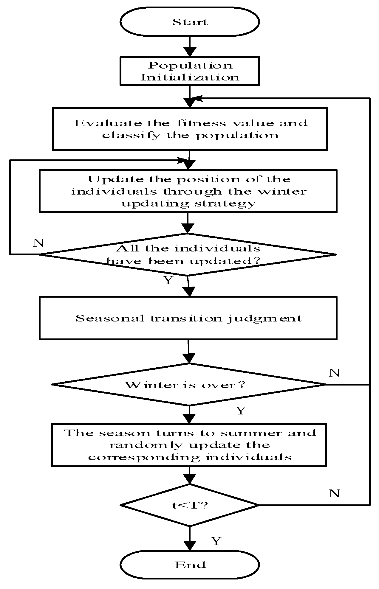
In conclusion, the procedure of the standard SSA is shown in Figure 1:
3. The improved Squirrel Search Algorithm
3.1. Motivation
A large number of experiments have proven that different evolutionary strategies are suitable for different problems, and also that the requirements are also different with the development of evolution. In the early stage of optimization, individuals are distributed dispersedly in the search space, and there are still large distances among the individuals with better fitness values. Thus it is important to maintain the diversity of the population to develop the search space sufficiently. Meanwhile, the convergence speed should be improved as well. In the later stage of optimization, the difference among the individuals are increasingly shorter, and thus the main work is to search around the elite individuals to improve the convergence speed. In addition to this, in order to prevent the algorithm from falling into a local optimal, the diversity of the population also needs to be supplemented.
Considering the analysis above, an improved squirrel search algorithm (ISSA) is proposed in this paper to improve the performance and the robustness of SSA. The proposed algorithm includes the jumping search method and the progressive search method, both of having an independent winter search strategy for the early evolutionary stage when and summer search strategy for the later evolutionary stage when . Algorithm 1 shows the detailed steps of ISSA:
| Algorithm 1. Pseudo Code of ISSA |
| Input:pop |
| Output:fbest (fbest is the best fitness value optimized by the algorithm) |
| for t = 1 to T (T is the total generation of the algorithm to be executed) |
| evaluate the fitness values of the population |
| update the population through the jumping search method introduced in Section 3.2 |
| if t == T/n (n is the total substages of the whole optimization, details in Section 3.4) |
| calculate the corresponding linear regression equations introduced in Section 3.4 |
| if two or more calculated slopes are positive |
| continue optimizing through the progressive search method introduced in Section 3.3 |
| else |
| continue optimizing through the jumping search method mentioned in Section 3.2 |
| end |
| end |
| end |
3.2. The Jumping Search Method
3.2.1. ‘Escape’ Operation in Winter
According to the winter updating method, a random relocation makes the endangered individuals abandon the current evolutionary direction, which decreases the convergence speed even if it can explore the new position to maintain the population diversity. In addition, the safe individuals evolve towards either Fh or Fa based on themselves, which can maintain the current evolutionary information and supplement the population diversity. However, the convergence speed will decrease because Fa is ultimately not the best individual.
In order to maintain the population diversity and improve the convergence speed, a new winter search strategy was designed in the jumping search method. The details are as follows:
If , FSi is safe, the position is updated by Formula (13):
If , FSi is endangered, FSi is considered to be dead and generates a new one by Formula (14):
In Formula (14), U is the maximum of FSi and L is the minimum of FSi.
Producing a subpopulation GS, all the individuals in GS have not been updated, and the original FSi is considered to be the predator with the hunting radius calculated by Formula (15). The individual in GS is threatened if the distance between itself and the predator is shorter than the hunting radius. All the threatened individuals ‘escape’ by Formula (16) and continue searching around the new position by Formula (17) after ‘escaping’.
In the formula above, FSj represents the threatened individual.
The advantages of the new winter search strategy include: (1) Considering the evolutionary information in early stage is abundant enough to maintain the population diversity, the safe individuals only evolve to the best individual Fh, which will improve the convergence speed; (2) The endangered individuals reinitialize in a smaller range, and thus the current evolutionary information can be retained in a way that avoids a blind search, which will improve the searching efficiency. More importantly, the threatened individuals evolve towards Fa which avoids the individuals concentrating excessively. The further development after ‘escaping’ supplements the population diversity and prevents the algorithm from falling into a local optimal. In summary, the new winter search strategy maintains the population diversity as well as improves the convergence speed, which satisfies the requirement of the early evolutionary stage.
3.2.2. ‘Death’ Operation in Summer
According to the summer updating method, only safe individuals who evolve towards Fa are randomly relocated; the others stay at their updated positions without any change, although it supplements the population diversity and retains the current evolutionary information, and the blindness of random relocation decreases the convergence speed, which is not fit for the requirement of the later evolutionary stage.
In order to satisfy the corresponding requirement, a new summer search strategy was proposed. The proposed strategy searches around the elite individual carefully and supplements the population diversity to make up the disadvantages introduced above. The details are as follows:
If , FSi is safe, the position is updated by Formula (18):
If , FSi is endangered, FSi is considered to be dead and a new one will be generated by Formula (19). Furthermore, all the threatened individuals are considered to be dead and the new ones will be generated by Formula (20):
In the formula above, N (0,1) is a random number which obeys the standard normal distribution.
Fh is the best individual found so far. Formula (18) takes Fh as the base vector and takes the differential vector between Fh and FSi as the disturbance. Due to the fact that differences among the individuals in summer () are smaller than those in winter (), the essence of Formula (18) is to search finely around Fh and retain the current evolutionary information. In Formula (19), the random number is generated by scattered in [0.5−2,0.52] but close to 1 in greater possibilities, thus the individuals generated by Formula (19) are more similar to FSi, while the individuals generated by Formula (20) distribute in [0.5Fh,1.5Fh] uniformly. Therefore, the search space of Formulas (19) and (20) are smaller than the random relocation shown in Formula (10). In addition, Formula (19) pays more attention to retain the current evolutionary information and Formula (20) pays more attention to developing the search space.
3.2.3. Characters of the Jumping Search Method
According to the new winter search strategy introduced in Section 3.2.1 and the new summer search strategy introduced in Section 3.2.2: (1) If , the winter search strategy takes the FSi as the base vector and takes the differential vectors between Fh and FSi as the disturbance; the summer search strategy takes the Fh as the base vector and takes the differential vectors between Fh and FSi as the disturbance. As both of them evolve towards Fh, the difference between the winter search strategy and the summer search strategy is that the former focuses on maintaining the population diversity, while the latter focuses on improving the convergence speed. (2) If , the winter search strategy updates the individuals by changing the learning target and gets away from the current position, while the summer search strategy generates new individuals around FSi or Fh. In summary, the different requirements in different stages are satisfied by the coordination of the two search strategies. The pseudo code of the jumping search method is shown in Algorithm 2:
| Algorithm 2. Pseudo Code of the Jumping Search Method |
| Input:pop |
| Output:popnew |
| if |
| season = winter |
| else |
| season = summer |
| end |
| if season == winter |
| forp1 = 1 to popsize (popsize is the total number of squirrels) |
| if |
| end |
| if |
| for p2 = 1 to nt1 (nt1 is the total number of threatened squirrels) |
| end |
| end |
| end |
| end |
| if season == summer |
| forp1 = 1 to popsize |
| if |
| end |
| if |
| for p2 = 1 to nt2 (nt2 is the total number of dead squirrels) |
| end |
| end |
| end |
3.3. The Progressive Search Method
3.3.1. The Principle of the Progressive Search Method
The progressive search method is designed to improve the robustness of SSA, compared with the jumping search method. The progressive search method has a similar thought but different details.
When , the season is winter, update and mutate the individuals as follows:
If , FSi is safe, update the position according to Formula (13);
If FSi is endangered, select a dimension randomly and mutate it in the range of FSL and FSH, which is aimed at retaining the current evolutionary direction and information.
When , the season is summer, update and mutate the individuals as follows:
If , FSi is safe, update the position according to Formula (21):
is calculated by Formulas (11) and (12), which makes the individuals search in a short distance with greater possibilities and search in a long distance occasionally.
If , FSi is endangered, select a dimension randomly and mutate it in the range of L and U.
3.3.2. The Analysis of the Progressive Search Method
According to the introduction of the progressive search method above, for the winter stage, if the individuals are safe, the search strategy is the same as that in the jumping search method. However, if the individuals are endangered, mutate one dimension of the individuals randomly, and the convergence speed will slow down but more evolutionary information is retained. For the summer stage, if the individuals are safe, the search strategy is similar to the jumping search method, but the gliding step is replaced by the flight. If the individuals are endangered, mutate one dimension of the individuals randomly to maintain the diversity of the population. Algorithm 3 shows the pseudo code of the progressive search method:
| Algorithm 3. Pseudo Code of the Progressive Search Method |
| Input:pop |
| Output:popnew |
| if |
| if |
| season = winter |
| else |
| season = summer |
| end |
| if season == winter |
| forp1 = 1 to popsize |
| end |
| if |
| select one dimension randomly and change it between FSL and FSH |
| end |
| end |
| end |
| if season == summer |
| forp1 = 1 to popsize |
| if |
| end |
| if |
| select one dimension randomly and change it between U and L |
| end |
| end |
3.4. Linear Regression Selection Strategy
According to the introduction in Section 3.2 and Section 3.3, due to the fact that individuals generated in summer are more similar to Fh, the jumping search method improves the convergence speed in an obvious manner. As the progressive search method retains the evolutionary information efficiently, the population diversity can be better maintained. Meanwhile, during the optimization process of the minimization problem, the best fitness value of the population is supposed to be a downward trend. If the population diversity is not abundant enough, the search space will not be developed sufficiently, meaning the algorithm will not convergence efficiently and the best fitness value will fluctuate or even become larger. Considering that different problems are suitable for different evolutionary strategies, this paper proposes a linear regression selection strategy to choose the appropriate updating method from the two methods mentioned above. The details are as follows:
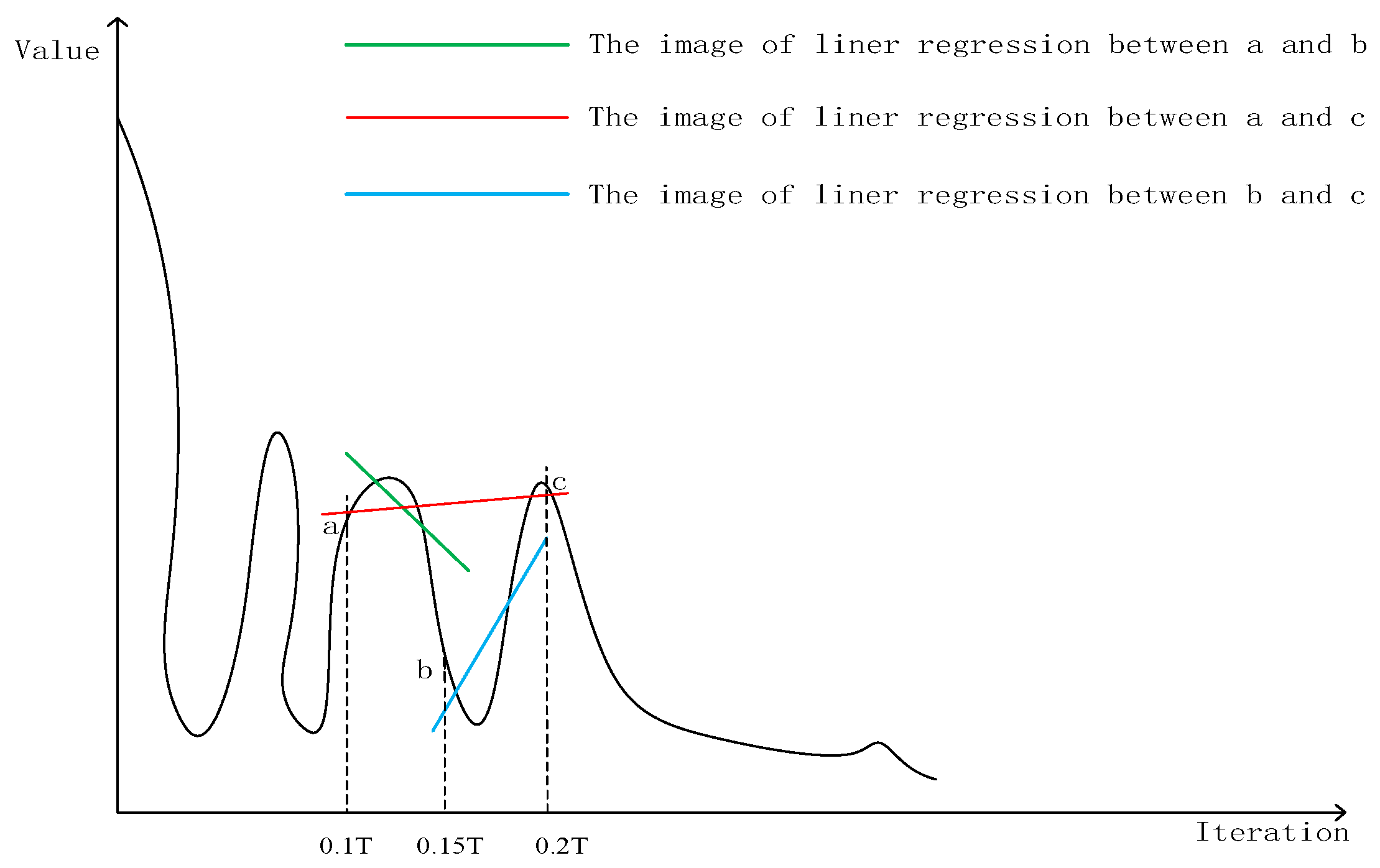
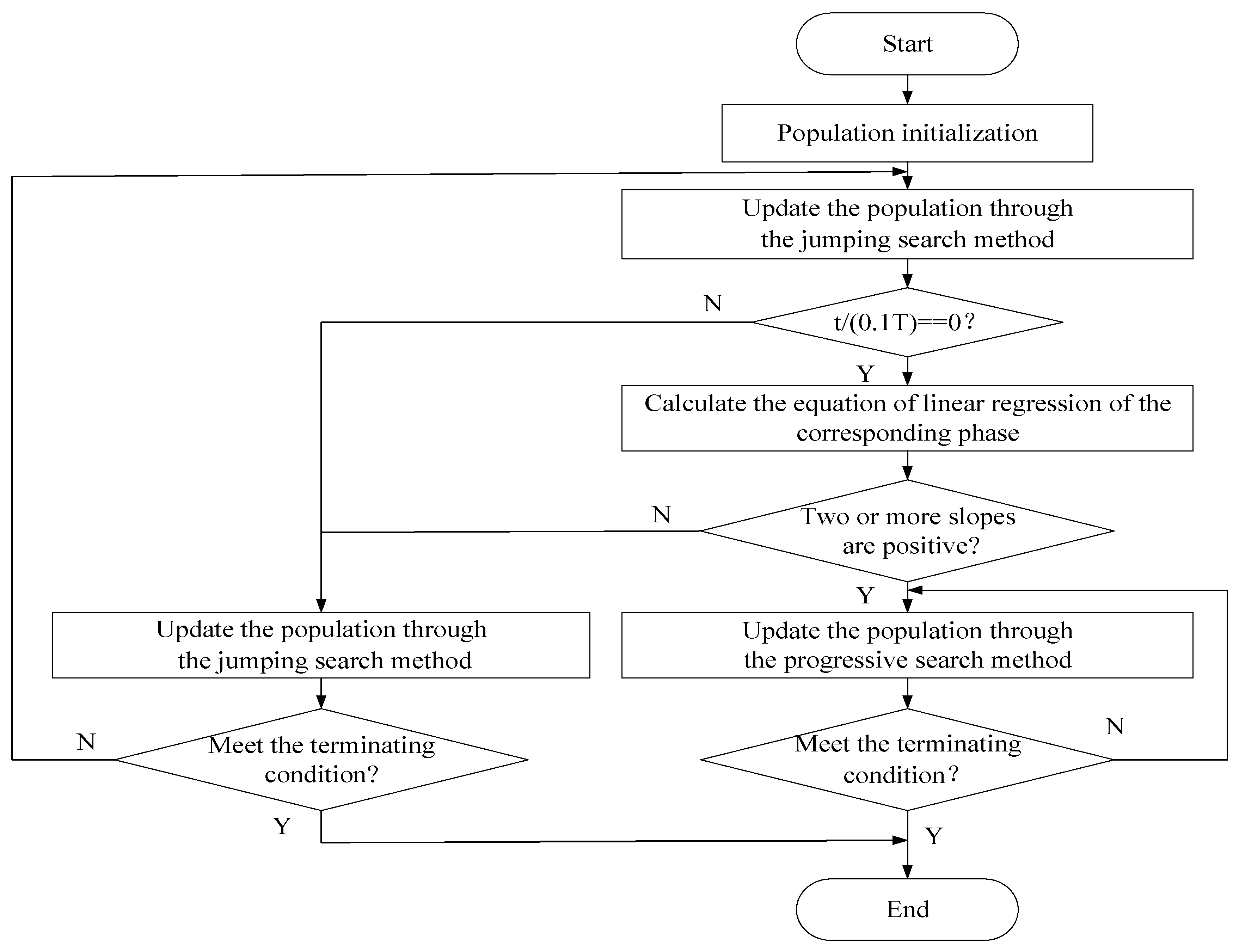
Divide the whole evolutionary process into n substages evenly. The optimization starts with the jumping search method, calculating the linear regression equations of the best fitness value when a substage is finished. There are three linear regression equations needed to be calculated: the best fitness value of the first half substage, the second half substage and the whole substage. If two or more equations’ slopes are positive, the best fitness value may fluctuate or become larger, that is, the population diversity needs to be supplemented. The jumping search method is not suitable for the current problem. Therefore, the progressive search method is selected to finish the evolution. Otherwise, the population diversity is abundant enough, and will continue evolving through the jumping search method to converge faster. Figure 2 is the illustration of the linear regression selection strategy introduced above. Taking n = 10 and t = 0.2 T as an example, calculate the linear regression equations of the three regions: [0.1 T, 0.15 T], [0.15 T, 0.2 T] and [0.1 T, 0.2 T]. It can be seen from Figure 2 that the slope of ab is negative, and the slopes of bc and ac are positive, which means that the best fitness value will fluctuate or become larger, therefore, select the progressive search method to finish the evolution. Figure 3 is the procedure of ISSA.
4. Analysis of the Experimental Results
4.1. Benchmark Functions
In order to test the performance of the proposed ISSA, a series of experiments are carried out. All the experiments work on CPU: Intel Core i5-7200 M, 4 G RAM, 2.70 GHZ, Windows 10 and Matlab R2016a.
The experiment selects 21 benchmark functions from reference [15,33,34,35], which include the low dimensional unimodal functions (F1, F2), the low dimensional multimodal functions (F3–F10), the high dimensional unimodal functions (F11–F17) and the high dimensional multimodal functions (F18–F21). The specific functions are shown in Table 1:
4.2. The Influence of Parameter on ISSA
ISSA divides the whole evolutionary process into n substages and selects the proper strategy when a substage is completed. In order to obtain good performances as fast as possible, take n = 0, n = 5, n = 10, n = 15 and n = 20 and test the ISSA on low dimensional unimodal function F2, the low dimensional multimodal functions F6 and F10, the high dimensional unimodal functions F16 and F17, the high dimensional multimodal functions F18 and the total number of evolutions at 18,000, respectively. Nfs is 3 which is the same as the reference [30]. The population size is 30, and every function runs 30 times independently in order to avoid the occasionality of the single execution. The results are as follows: the number before ‘±’ is the mean and the number after ‘±’ is the deviation of the obtained best fitness value.
According to Table 2, there is almost no impact of different n on low dimensional unimodal function; for low dimensional multimodal functions, the results of n = 0 are much worse than that of n ≠ 0. According to 3.4, ISSA starts with the jumping search method and ISSA is same as the jumping search method in total when n = 0. ISSA is the combination of two strategies and the searching strategy may turn to the progressive search method when n ≠ 0. The results of F2 and F6 mean that different strategies are fit for different problems and the linear regression selection strategy is effective. Aside from this, the results of F2 and F6 are better with a higher selection frequency; for high dimensional unimodal functions, the experimental results are not much different. However, there are obvious differences on a high dimensional multimodal function between n = 5 and n = 0, n = 10, 15 and 20. In order to guarantee the convergence performance and the operating efficiency of ISSA at the same time, take n = 10 for the remaining experiments in this paper.
4.3. The Efficiency of the Proposed Methods
The proposed ISSA selects the jumping search method or the progressive method according to the linear regression selection strategy automatically. In order to verify the efficiency of the proposed methods, compare the standard SSA, the jumping search method, the progressive method and the ISSA through the 21 benchmark functions in terms of convergence speed, population diversity and convergence precision.
4.3.1. Comparison of Convergence Speed on Four Methods
For each method mentioned above, the total number of evolution is 30,000 and Nfs is 3, the population size is 30, which is aimed at comparing the methods fairly effectively. Every method runs 30 times independently in order to avoid the randomness of the single execution.
Figure 4a–i shows the convergence curves of SSA, the jumping search method, the progressive search method and ISSA on the low dimensional unimodal functions F2, the low dimensional multimodal functions F3 and F5, the high dimensional unimodal functions F11, F13, F14 and F16 and the high dimensional multimodal functions F18 and F21 when the evaluation time is 30,000. The blue, green, yellow and red curves refer to SSA, the jumping search method, the progressive method and ISSA, respectively. The abscissa of each figure is the iteration and the ordinate of each figure is the best value found so far. The title of each figure is given as the name F2, F3, F5, F11, F13, F14 and F16. For the low dimensional functions, the jumping search method, the progressive method and ISSA all have obvious improvements on convergence speed compared with SSA. The convergence speed from high to low is the jumping search method, ISSA and the progressive search method. In relation to the high dimensional functions, the convergence speed of the jumping search method and ISSA is still much better than SSA and the jumping search method performs better, but the improvement of the progressive search method is not as obvious as that on the low dimensional functions.
4.3.2. Comparison of Population Diversity on Four Methods
In order to compare the population diversity of the four methods intuitively, all the population sizes are 30. Table 3 is the comparison of the individuals’ distribution on the 2-dimensional unimodal function F2 and the 2-dimensional multimodal function F5 when the convergence accuracy is up to 10−6, 10−8 and 10−10. The points in the figures refer to the individuals’ positions, and the blue, green, black and red points refer to SSA, the jumping search method, the progressive search method and ISSA, respectively. The abscissa and the ordinate of each figure are the search range for the function; for F2 the search range is from −10 to 10 and for F5 the search range is from −100 to 100. The title of each figure is the name of F2 or F5. Table 4 shows the variance of the population’s fitness values when the algorithms converge to about 10−4 of benchmark functions. The functions contain the high dimensional unimodal functions F11 and F12 and the high dimensional multimodal functions F20 and F21. The number before ‘±’ is the variance’s mean and the number after ‘±’ is the variance’s standard deviation. ‘/’ represents the algorithm failure to converge to 10−4 after evaluating 30,000 times.
It can be seen from Table 3 that SSA has the most dispersed individual distribution because of the individuals’ re-initialization. For the three proposed strategies mentioned in this paper, individuals of the progressive search method distribute most dispersedly. ISSA takes second place, and the jumping search method has the most concentrated distribution. The progressive search method mutates individuals on a certain dimension, which will make more individuals distribute on lines x1 = 0 and x2 = 0. As a result, the benchmark functions have a great chance to converge to the optimal value. SSA re-initializes the whole individual, which makes the individuals distribute in the search space irregularly. From the analysis above, the progressive search method has the best population diversity while the jumping search method performs worst when the population evaluates to the fixed accuracy.
Data in Table 4 show that the variances of SSA and the progressive search method are much larger than the variances of the jumping method and ISSA. Excessive population diversity slows down the convergence speed and some functions cannot converge to the fixed accuracy. Meanwhile, for the population diversity of the three proposed strategies in this paper, the progressive search method performs best, ISSA takes second place and the jumping search method performs worst.
4.3.3. Comparison of Comprehensive Performance on Four Methods
In order to compare the comprehensive performance of the four methods, Table 5 shows the mean and standard deviation of the optimal value obtained in 30 independent experiments on the 21 benchmark functions. For each method, the population size is 30, the total of evolution times is 30,000 and the Nfs is 3. The number before ‘±’ is the mean and the number after ‘±’ is the deviation of the obtained best fitness value; ‘+’, ‘−’ and ‘=’ represent that the means of the corresponding method are better than ISSA, worse than ISSA and equal to ISSA, respectively.
Table 5 shows that the convergence precision of the jumping search method, the progressive method and the ISSA are all obviously better than SSA. Meanwhile, compared with ISSA, the numbers of benchmark functions with the better mean, the worse mean and the equivalent mean of SSA are 1, 18, and 2, respectively; the corresponding numbers of the jumping search method are 1, 4 and 16, respectively; the corresponding numbers of the progressive search method are 3, 12 and 6, respectively. In order to compare the differences of each method, a Friedman test was taken to check the data in Table 5 [36]. The specific process is shown below:
The Friedman test ranks the algorithms for each data set separately; k refers to the number of algorithms and n refers to the number of data sets of each algorithm. The results are shown in Table 6, and is calculated as follows: ; α = 0.05, df = 4 − 1 = 3 at the 5% significant level and according to the Chi-square distribution table. Therefore, the four methods are considered to have significant differences at the 5% significance level.
To further compare the performance of the four methods, assuming that the convergence performance of ISSA is better than the other three methods, a Holm test was carried out and the results are shown in Table 7:
It can be seen from Table 7 that , , . The original hypothesis is rejected at the 5% significance level. Therefore, compared with SSA, ISSA has significantly better performance. ISSA has a smaller average rank, though it does not outperform the progressive search method and the jumping search method.
In conclusion, the jumping search method has the best convergence speed and the progressive search method performs best on maintaining the population diversity. Compared with SSA, both have obvious advantages in convergence accuracy. ISSA combines the two methods together, improves the convergence speed and the convergence accuracy and maintains the population diversity as well. ISSA can find the global optimal of more benchmark functions and has the best comprehensive performance.
4.4. Performance Compared with Other Algorithms
To verify the advantages of ISSA, we compared it with five algorithms with better optimization results: the improved differential evolutionary algorithm—MDE (modified differential evolution, with self-adaptive parameters method) [37], the improved gravitational search algorithm—IGSA/PSO (an improved gravitational search algorithm for green partner selection in virtual enterprises) [38], the improved artificial bee colony algorithm—distABC (artificial bee colony algorithm, with distribution-based update rule) [39], the improved particle swarm optimization—ADN-RSN-PSO (all-dimension neighborhood based particle swarm optimization with randomly selected neighbors) [40] and the improved grey wolf optimization algorithm—PSO-GWO (an improved hybrid grey wolf optimization algorithm) [41].
For each algorithm mentioned above, the population number is 30, the total number of evolution times is 24,000 and each method runs 30 times independently to ensure the comparison is fair enough. The relevant parameters are set as follows:
- ISSA: n = 10; Nfs = 3;
- MDE: the crossover probability CR = 0.4, the mutation probability F is determined by the random number between 0 and 1.
- IGSA/PSO: the gravitational constant G0 = 100, α = 20;
- distABC: limit = (the population number × dimension)/2;
- ADN-RSN-PSO: the weight factor w = 0.7298, c1 = c2 = 2.05;
- PSO-GWO: the weight factor c1 = c2 = 2.05; aini = 2, afin = 0; r1, r2, r3, r4 are all the random numbers between 0 and 1.
Table 8 shows the optimization results of low dimensional functions (F1–F10) and Table 11 shows the ones of high dimensional functions (F11–F21). Best, Worst, Mean and SD respectively represent the best fitness value, the worst fitness value, the mean fitness value and the standard deviation obtained by 30 independent executions. R represents the times of the algorithm converges to the appointed precision. The appointed precision is 10−8 for the benchmark functions, whose optimal is 0. For the benchmark functions F1, F7, F9 and F10 whose optimal is not equal to 0, the appointed precision is −0.6, −1.6, −3.6 and −8.6 respectively.
It can be seen from Table 8 that MDE can converge to the optimal on F1, F3, F4, F5, F6, F7 and F8, but the performances of F7 and F8 are not stable enough; distABC only converges to the optimal stably on F4 and has a certain probability to converge to the optimal on F3 and F5; IGSA/PSO has no stable convergence performance on all the functions but still has a certain probability to converge to the optimal on F1, F3, F4 and F5; ADN-RSN-PSO has the worst performance without any function convergences to the optimal; PSO-GWO can converge stably to the optimal on F3, F4, F5 and F8, and there is also a certain probability for F7 to converge to the optimal. For ISSA, all the low dimensional functions can converge to the optimal and have the stable convergence performances on F2, F3, F4, F5 and F8. Aside from this, ISSA obtains the minimum mean on all functions except F6. In order to compare the differences of each method, we used the Friedman test to check the data in Table 8. The specific process is shown below, and the results can be obtained by Table 9:
; α = 0.05, df = 6 − 1 = 5 at the 5% significant level and according to the Chi-square distribution table. Therefore, the six algorithms are considered to have significant differences at the 5% significance level.
To further compare the performance of the six algorithms, assume that the convergence performance of ISSA is better than the other five algorithms. A Holm test was carried out and the results are shown in Table 10:
It can be seen from Table 10 that , , , , ; the original hypothesis is rejected at the 5% significance level. Therefore, compared with AND-RSN-PSO, distABC and IGSA/PSO, ISSA has significantly better performance. ISSA has a smaller average rank, though it does not outperform PSO-GWO and MDE. In summary, compared with five other algorithms, the proposed algorithm ISSA has better performance on the low dimensional functions.
Table 11 shows the convergence results on the high dimensional functions. It can be seen that MDE can converge to a certain precision on F11, F12, F13, F16, F18 and F20, but the obtained precision has obvious gaps compared with ISSA; distABC almost has no efficient convergence performance on the high dimensional functions; IGSA/PSO can converge to a certain precision on F11, F12 and F13, but the results are not good enough; ADN-RSN-PSO can converge to a certain precision on all the high dimensional functions except on F18, but the obtained precision is far from ISSA; PSO-GWO can converge to a better precision except on F18, whose convergence result is not good enough and on F21 which cannot converge efficiently, with the obtained convergence precision still being worse than that of ISSA. For ISSA, all the functions can converge to the optimal except F15, F16 and F20. Aside from this, the best fitness value, the worst fitness value, the mean fitness value and the standard deviation of F11, F12, F13, F14, F17, F19 and F21 are all equal to zero and keep unchanged even if the dimensions become higher. The best fitness value of F18 is also equal to zero no matter whether the dimension is 30, 50 or 100, and the deviation is much smaller than the other five algorithms for F15, F16 and F20, which cannot converge to the optimal. The best fitness value, the worst fitness value, the mean fitness value and the standard deviation are still much better than the other five algorithms. In order to compare the differences of each method, a Friedman test is taken to check the data in Table 11 when the dimension is 30. The specific process is shown below:
It can be obtained by: with the results shown in Table 12; α = 0.05, df = 6 − 1 = 5 at the 5% significant level and according to the Chi-square distribution table. Therefore, the six algorithms are considered to have significant differences at the 5% significance level.
To further compare the performance of the six algorithms, assume that the convergence performance of ISSA is better than the other five methods. A Holm test is carried out and the results are shown in Table 13:
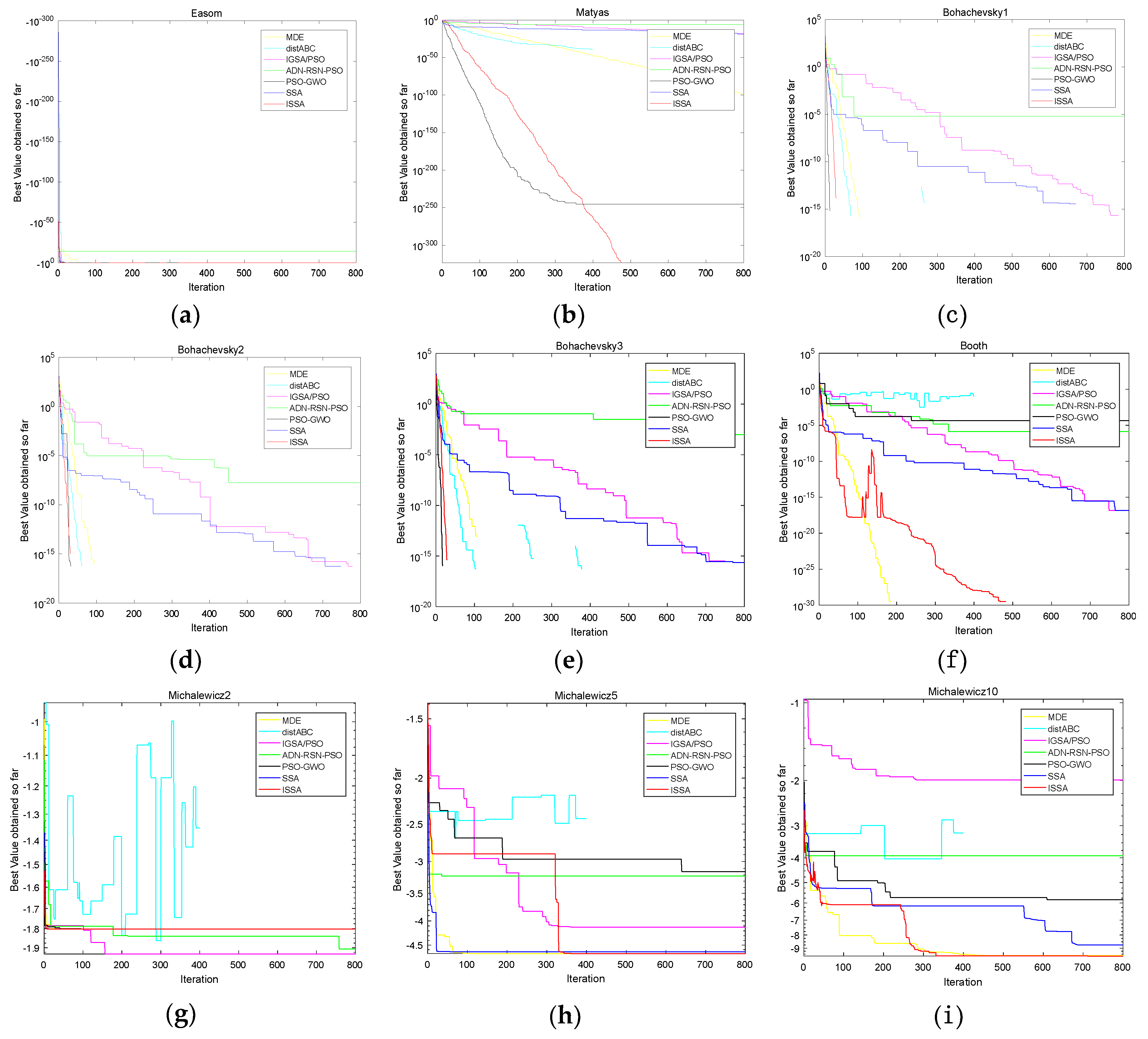
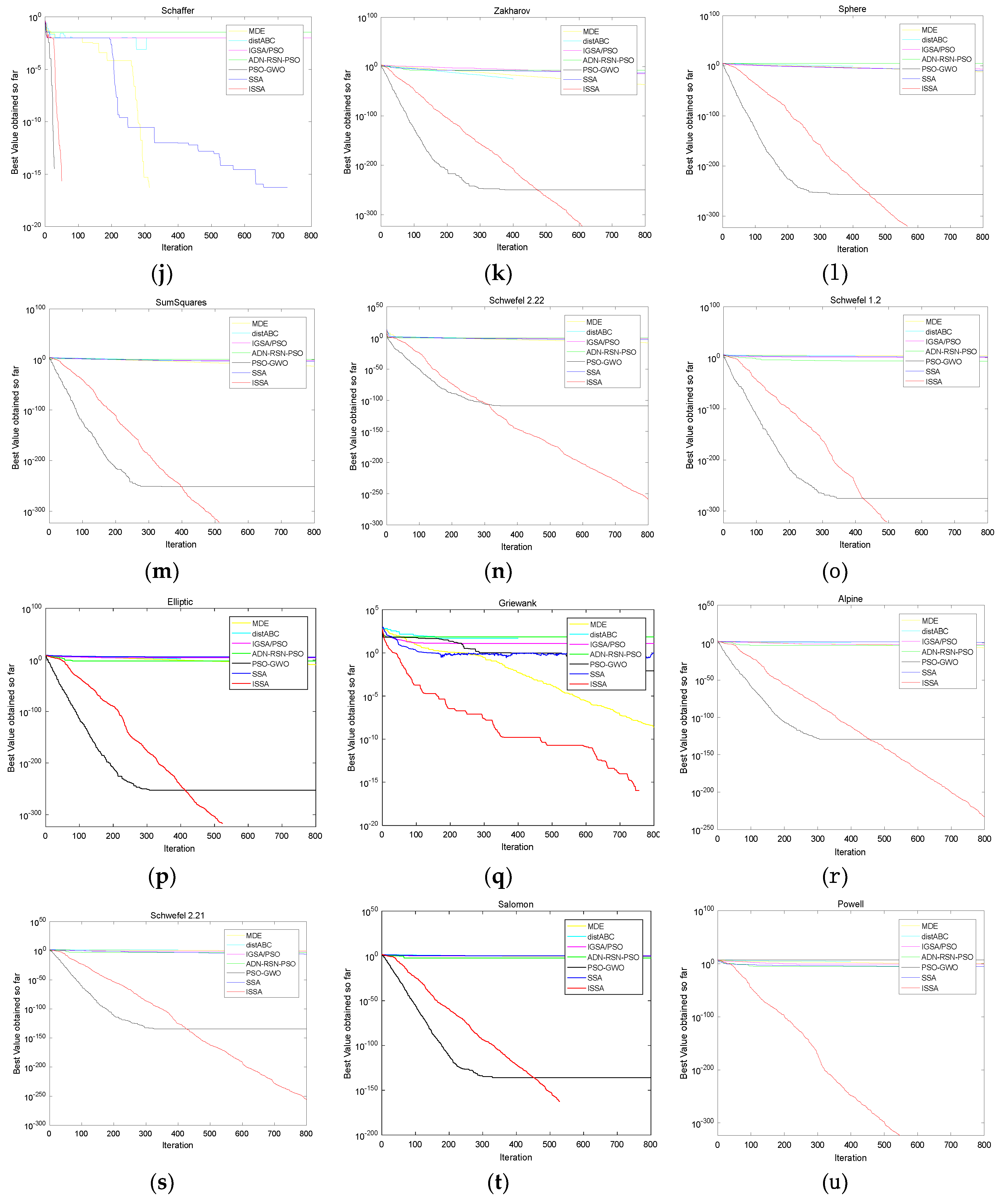
It can be seen from Table 13 that , , , , , and the original hypothesis is rejected at the 5% significance level. Therefore, compared with AND-RSN-PSO, distABC, IGSA/PSO and MDE, ISSA has a significantly better performance. ISSA has a smaller average rank, though it does not outperform PSO-GWO. In summary, the ISSA proposed in this paper has obvious advantages on convergence precision and stability in terms of the high dimensional functions. Figure 5a–u shows the convergence curves of the algorithms mentioned above on F1–F21 in order to compare the convergence performances intuitively. The yellow, cyan, purple, green, black, blue and red curves refer to MDE, distABC, IGSA/PSO, AND-RSN-PSO, PSO-GWO, SSA and ISSA, respectively. The abscissa of each figure is the iteration and the ordinate of each figure and is the best value found so far. The title of each figure is given the name of F1–F21.
5. Conclusions
This paper proposes an improved squirrel search algorithm. In terms of SSA, the winter searching method cannot develop the search space sufficiently, and the summer searching method is too random to guarantee the convergence speed. ISSA introduces the jumping search method and the progressive search method. For the jumping search method, the ‘escape’ operation in winter supplements the population diversity and fully exploits the search space, while the ‘death’ operation in summer explores the search space more sufficiently and improves the convergence speed. Aside from this, the mutation in the progressive search method retains the evolutionary information more effectively and maintains the population diversity. ISSA selects the suitable method by the linear regression selection strategy according to the variation tendency of the best fitness value, which improves the robustness of the algorithm. Compared with SSA, ISSA pays more attention to developing the search space in winter, and pays more attention to exploring around the elite individual in summer, which keeps a good balance between development and exploration improves the convergence speed and the convergence accuracy. Moreover, ISSA selects a proper search strategy along with the optimization processing, so ISSA has greater possibilities in finding the optimal solution. The experimental results on 21 benchmark functions and the statistical tests show that the proposed algorithm can promote the convergence speed, improve the convergence accuracy and maintain the population diversity at the same time. Furthermore, ISSA has obvious advantages in convergence performances compared with other five intelligent evolutionary algorithms.
Author Contributions
Y.J.W. designed the experiments and revised the paper; T.L.D. shared the ideas and mainly wrote the paper.
Funding
This research was funded by the National Natural Science Foundation of China under grants NO.61501107 and NO.61603073, and the Project of Scientific and Technological Innovation Development of Jilin NO.201750227 and NO.201750219.
Conflicts of Interest
The authors declare no conflict of interest.
References
- He, J.; Lin, G. Average Convergence Rate of Evolutionary Algorithms. IEEE Trans. Evol. Comput. 2016, 20, 316–321. [Google Scholar] [CrossRef]
- Chugh, T.; Sindhya, K.; Hakanen, J. A survey on handling computationally expensive multiobjective optimization problems with evolutionary algorithms. Soft Comput. 2017, 23, 3137–3166. [Google Scholar] [CrossRef]
- Bhattacharyya, B.; Raj, S. Swarm intelligence based algorithms for reactive power planning with Flexible AC transmission system devices. Int. J. Electr. Syst. 2016, 78, 158–164. [Google Scholar] [CrossRef]
- Laina, R.; Lamzouri, F.E.-Z.; Boufounas, E.-M.; El Amrani, A.; Boumhidi, I. Intelligent control of a DFIG wind turbine using a PSO evolutionary algorithm. Procedia Comput. Sci. 2018, 127, 471–480. [Google Scholar] [CrossRef]
- Manjunath, P.G.C.; Krishna, P.; Parappagoudar, M.B.; Vundavilli, P.R. Multi-Objective Optimization of Squeeze Casting Process using Evolutionary Algorithms. IJSIR 2016, 7, 55–74. [Google Scholar]
- Ntouni, G.D.; Paschos, A.E.; Kapinas, V.M.; Karagiannidis, G.K.; Hadjileontiadis, L.J. Optimal detector design for molecular communication systems using an improved swarm intelligence algorithm. Micro Nano Lett. 2018, 13, 383–388. [Google Scholar] [CrossRef]
- Liu, M.; Zhang, F.; Ma, Y.; Pota, H.R.; Shen, W. Evacuation path optimization based on quantum ant colony algorithm. Adv. Eng. Inform. 2016, 30, 259–267. [Google Scholar] [CrossRef]
- Yang, J.H.; Honavar, V. Feature Subset Selection Using a Genetic Algorithm. IEEE Intell. Syst. 1998, 13, 44–49. [Google Scholar] [CrossRef]
- Storn, R.; Price, K. Differential Evolution—A Simple and Efficient Heuristic for global Optimization over Continuous Spaces. J. Glob. Optim. 1997, 11, 341–359. [Google Scholar] [CrossRef]
- Hansen, N.; Ostermeier, A. Completely Derandomized Self-Adaptation in Evolution Strategies. Evol. Comput. 2001, 9, 159–195. [Google Scholar] [CrossRef] [Green Version]
- De Castro, L.N.; Von Zuben, F.J. Learning and Optimization Using the Clonal Selection Principle. IEEE Trans. Evol. Comput. 2002, 6, 239–251. [Google Scholar] [CrossRef]
- Xie, X.F.; Zhang, W.J.; Yang, Z.L. Social cognitive optimization for nonlinear programming problems. In Proceedings of the 2002 International Conference on Machine Learning and Cybernetics, Beijing, China, 4–5 November 2002; pp. 779–783. [Google Scholar]
- Ashrafi, S.M.; Dariane, A.B. A novel and effective algorithm for numerical optimization: Melody Search (MS). In Proceedings of the 2011 11th International Conference on Hybrid Intelligent Systems, Malacca, Malaysia, 5–8 December 2011; pp. 109–114. [Google Scholar]
- Rao, R.V.; Patel, V. An elitist teaching-learning-based optimization algorithm for solving complex constrained optimization problems. Int. J. Ind. Eng. Comput. 2012, 3, 535–560. [Google Scholar] [CrossRef]
- Cheng, M.Y.; Prayogo, D. Symbiotic Organisms Search: A new metaheuristic optimization algorithm. Comput. Struct. 2014, 139, 98–112. [Google Scholar] [CrossRef]
- Jahani, E.; Chizari, M. Tackling global optimization problems with a novel algorithm—Mouth Brooding Fish algorithm. Appl. Soft Comput. 2018, 62, 987–1002. [Google Scholar] [CrossRef]
- Kirkpatrick, S.; Gelatt, C.D., Jr.; Vecchi, M.P. Optimization by Simulated Annealing. Science 1983, 220, 671–680. [Google Scholar] [CrossRef] [Green Version]
- Rashedi, E.; Nezamabadi-Pour, H.; Saryazdi, S. GSA: A Gravitational Search Algorithm. Inf. Sci. 2009, 179, 2232–2248. [Google Scholar] [CrossRef]
- Mirjalili, S.; Sadiq, A.S. Magnetic Optimization Algorithm for training Multi Layer Perceptron. In Proceedings of the IEEE 3rd International Conference on Communication Software and Networks, Xi’an, China, 27–29 May 2011; pp. 42–46. [Google Scholar]
- Kaveh, A.; Khayatazad, M. A new meta-heuristic method: Ray Optimization. Comput. Struct. 2012, 112–113, 283–294. [Google Scholar] [CrossRef]
- Moein, S.; Logeswaran, R. KGMO: A swarm optimization algorithm based on the kinetic energy of gas molecule. Inf. Sci. 2014, 275, 127–144. [Google Scholar] [CrossRef]
- Kaveh, A.; Bakhshpoori, T. Water Evaporation Optimization: A novel physically inspired optimization algorithm. Comput. Struct. 2016, 167, 69–85. [Google Scholar] [CrossRef]
- Nematollahi, A.F.; Rahiminejad, A.; Vahidi, B. A novel physical based meta-heuristic optimization method known as Lightning Attachment Procedure Optimization. Appl. Soft Comput. 2017, 59, 596–621. [Google Scholar] [CrossRef]
- Colorni, A. Distributed Optimization by Ant Colonies. In Proceedings of the 1st European Conference on Artificial Life, Paris, France, 11–13 December 1991; pp. 134–142. [Google Scholar]
- Kennedy, J.; Eberhart, R.C. Particle swarm optimization. In Proceedings of the IEEE International Conference on Neural Networks, Perth, Australia, 27 November–1 December 1995; pp. 1942–1948. [Google Scholar]
- Basturk, B.; Karaboga, D. An artificial bee colony (ABC) algorithm for numeric function optimization. In Proceedings of the Swarm Intelligence Symposium, Indianapolis, IN, USA, 12–14 May 2006; pp. 687–697. [Google Scholar]
- Cuevas, E.; Cienfuegos, M. A swarm optimization algorithm inspired in the behavior of the social-spider. Expert. Syst. Appl. 2013, 40, 6374–6384. [Google Scholar] [CrossRef] [Green Version]
- Fausto, F.; Cuevas, E.; Valdivia, A. A global optimization algorithm inspired in the behavior of selfish herds. Biosystems 2017, 160, 39–55. [Google Scholar] [CrossRef] [PubMed]
- Zhang, Z.; Huang, C.; Huang, H.; Tang, S.; Dong, K. An optimization method: Hummingbirds optimization algorithm. J. Syst. Eng. Electron. 2018, 29, 168–186. [Google Scholar] [CrossRef]
- Jain, M.; Singh, V.; Rani, A. A novel nature-inspired algorithm for optimization: Squirrel search algorithm. Swarm Evol. Comput. 2018, 44, 148–175. [Google Scholar] [CrossRef]
- Zhang, Y.; Liu, M. An improved genetic algorithm encoded by adaptive degressive ary number. Soft Comput. 2018, 22, 6861–6875. [Google Scholar] [CrossRef]
- Gomes, W.C.; dos Santos Filho, R.C.; de Sales Junior, C.D.S. An Improved Artificial Bee Colony Algorithm with Diversity Control. In Proceedings of the 2018 Brazilian Conference on Intelligent Systems, Sao Paulo, Brazil, 22–25 October 2018; pp. 19–24. [Google Scholar]
- Wang, S.; Li, Y.; Yang, H. Self-adaptive differential evolution algorithm with improved mutation strategy. Appl. Intell. 2017, 47, 644–658. [Google Scholar] [CrossRef]
- Kiran, M.S.; Hakli, H.; Gunduz, M. Artificial bee colony algorithm with variable search strategy for continuous optimization. Inf. Sci. 2015, 300, 140–157. [Google Scholar] [CrossRef]
- Feng, X.; Xu, H.; Wang, Y. The social team building optimization algorithm. Appl. Soft Comput. 2018, 2, 1–22. [Google Scholar] [CrossRef]
- Demišar, J.; Schuurmans, D. Statistical Comparisons of Classifiers over Multiple Data Sets. J. Mach. Learn. Res. 2006, 7, 1–30. [Google Scholar]
- Li, X.; Yin, M. Modified differential evolution with self-adaptive parameters method. J. Comb. Optim. 2016, 31, 546–576. [Google Scholar] [CrossRef]
- Xiao, J.; Niu, Y.; Chen, P. An improved gravitational search algorithm for green partner selection in virtual enterprises. Neurocomputing 2016, 217, 103–109. [Google Scholar] [CrossRef]
- Babaoglu, I. Artificial bee colony algorithm with distribution-based update rule. Appl. Soft Comput. 2015, 34, 851–861. [Google Scholar] [CrossRef]
- Sun, W.; Lin, A.; Yu, H. All-dimension neighborhood based particle swarm optimization with randomly selected neighbors. Inf. Sci. 2017, 405, 141–156. [Google Scholar] [CrossRef]
- Teng, Z.J.; Lv, J.L.; Guo, L.W. An improved hybrid grey wolf optimization algorithm. Soft Comput. 2018, 22, 1–15. [Google Scholar] [CrossRef]
Figure 1.
The procedure of the standard squirrel search algorithm (SSA).

Figure 2.
The illustration of the linear regression selection strategy.

Figure 3.
The procedure of improved squirrel search algorithm (ISSA).

Figure 4.
Convergence curves of the proposed methods and SSA.

Figure 5.
The convergence curves of ISSA and other algorithms.


Table 1.
Benchmark functions.
| Name | Function | D | Range | Optimal |
|---|---|---|---|---|
| F1 Easom | 2 | [−100,100] | −1 | |
| F2 Matyas | 2 | [−10,10] | 0 | |
| F3 Bohachevsky1 | 2 | [−100,100] | 0 | |
| F4 Bohachevsky2 | 2 | [−100,100] | 0 | |
| F5 Bohachevsky3 | 2 | [−100,100] | 0 | |
| F6 Booth | 2 | [−10,10] | 0 | |
| F7 Michalewicz2 | 2 | −1.8013 | ||
| F8 Schaffer | 2 | [−100,100] | 0 | |
| F9 Michalewicz5 | 5 | −4.6877 | ||
| F10 Michalewicz10 | 10 | −9.6602 | ||
| F11 Zakharov | 30/50/100 | [−5,10] | 0 | |
| F12 Sphere | 30/50/100 | [−100,100] | 0 | |
| F13 SumSquares | 30/50/100 | [−10,10] | 0 | |
| F14 Schwefel 1.2 | 30/50/100 | [−100,100] | 0 | |
| F15 Schwefel 2.21 | 30/50/100 | [−100,100] | 0 | |
| F16 Schwefel 2.22 | 30/50/100 | [−10,10] | 0 | |
| F17 Elliptic | 30/50/100 | [−100,100] | 0 | |
| F18 Griewank | 30/50/100 | [−600,600] | 0 | |
| F19 Salomon | 30/50/100 | [−100,100] | 0 | |
| F20 Alpine | 30/50/100 | [−10,10] | 0 | |
| F21 Powell | 32/52/100 | [4,5] | 0 |
Table 2.
The experimental results of ISSA with different n.
| F | n | ||||
|---|---|---|---|---|---|
| 0 | 5 | 10 | 15 | 20 | |
| F2 | 0 ± 0 | 0 ± 0 | 0 ± 0 | 0 ± 0 | 0 ± 0 |
| F6 | 6.2502e−04 ± 1.9021e−04 | 1.7129e−10 ± 9.2634e−11 | 3.5323e−08 ± 1.2626e−09 | 7.7188e−07 ± 2.8698e−08 | 7.5656e−07 ± 1.9151e−08 |
| F10 | −7.6632 ± 0.7985 | −9.4261 ± 0.0680 | −9.2260 ± 0.7780 | −8.1919 ± 1.3054 | −8.0299 ± 1.1781 |
| F16 | 6.2909e−163 ± 0 | 7.4432e−162 ± 0 | 1.0302e−164 ± 0 | 2.0455e−165 ± 0 | 7.1391e−164 ± 0 |
| F17 | 0 ± 0 | 0 ± 0 | 0 ± 0 | 0 ± 0 | 0 ± 0 |
| F18 | 1.8504e−15 ± 1.0135e−15 | 4.4095e−08 ± 1.9301e−07 | 2.1945e−15 ± 8.2481e−16 | 2.9976e−15 ± 6.5204e−15 | 3.1826e−15 ± 7.1639e−15 |
Table 3.
The comparison of the individuals’ distribution.
| Fun Accuracy | Method | ||||
|---|---|---|---|---|---|
| SSA | Jumping Search | Progressive Search | ISSA | ||
| F2 | 10−6 |  |  |  |  |
| 10−8 |  |  |  |  | |
| 10−10 |  |  |  |  | |
| F5 | 10−6 |  |  |  |  |
| 10−8 |  |  |  |  | |
| 10−10 |  |  |  |  | |
Table 4.
The comparison of the population’s fitness value.
| Name | Method | |||
|---|---|---|---|---|
| SSA | Jumping Search Method | Progressive Search Method | ISSA | |
| F11 | 1.2837e+05 ± 7.3449e+04 | 2.5981e−04 ± 2.4867e−04 | 1.1115e+04 ± 3.3201e+03 | 0.0017 ± 0.0015 |
| F12 | 5.7955e+04 ± 2.1202e+04 | 7.1891e−05 ± 4.6142e−05 | 1.3107e+03 ± 543.9195 | 7.2366e−04 ± 6.0848e−04 |
| F20 | / | 6.0584e−05 ± 2.5350e−05 | 1.2767 ± 0.2946 | 2.2921e−04 ± 1.7366e−04 |
| F21 | / | 8.5775e−05 ± 8.4886e−05 | 7.2621e+04 ± 6.0527e+04 | 6.2753e−04 ± 4.7156e−04 |
Table 5.
The comparison of the convergence precision.
| Name | Method | |||
|---|---|---|---|---|
| SSA | Jumping Search Method | Progressive Search Method | ISSA | |
| F1 | −1 ± 0 (=) | −1 ± 1.0909e−16 (=) | −1 ± 0 (=) | −1 ± 3.9171e−16 |
| F2 | 4.4212e−21 ± 1.5032e−20 (−) | 0 ± 0 (=) | 9.7986e−149 ± 5.3669e−148 (−) | 0 ± 0 |
| F3 | 7.4015e−18 ± 4.0540e−17 (−) | 0 ± 0 (=) | 0 ± 0 (=) | 0 ± 0 |
| F4 | 1.0191e−20 ± 2.9625e−20 (−) | 0 ± 0 (=) | 0 ± 0 (=) | 0 ± 0 |
| F5 | 1.2019e−20 ± 4.4285e−20 (−) | 0 ± 0 (=) | 0 ± 0 (=) | 0 ± 0 |
| F6 | 1.4402e−18 ± 3.0624e−18 (+) | 0.0202 ± 0.0238 (−) | 2.6295e−33 ± 1.4403e−32 (+) | 4.9331e−12 ± 1.6068e−11 |
| F7 | −1.8468 ± 0.0838 (−) | −1.7911 ± 0.0116 (−) | −1.8013 ± 6.8344e−16 (=) | −1.8013 ± 8.5739e−16 |
| F8 | 0 ± 0 (=) | 0 ± 0 (=) | 0 ± 0 (=) | 0 ± 0 |
| F9 | −4.6459 ± 2.7201e−15 (−) | −4.4543 ± 0.1818 (−) | −4.6808 ± 0.1336 (+) | −4.6617 ± 0.0304 |
| F10 | −9.5333 ± 0.2598 (−) | −8.2037 ± 0.3744 (−) | −9.6602 ± 0 (+) | −9.5882 ± 0.0891 |
| F11 | 2.7472e−13 ± 1.1640e−12 (−) | 0 ± 0 (=) | 2.1318e−16 ± 1.1676e−15 (−) | 0 ± 0 |
| F12 | 8.0478e−13 ± 4.3612e−12 (−) | 0 ± 0 (=) | 1.9301e−15 ± 1.0572e−14 (−) | 0 ± 0 |
| F13 | 2.0435e−10 ± 1.0129e−09 (−) | 0 ± 0 (=) | 3.5232e−11 ± 1.9297e−10 (−) | 0 ± 0 |
| F14 | 0.5472 ± 2.7161 (−) | 0 ± 0 (=) | 0.0865 ± 0.4149 (−) | 0 ± 0 |
| F15 | 7.2194e−08 ± 6.4247e−08 (−) | 0 ± 0 (=) | 0.0241 ± 0.1321 (−) | 0 ± 0 |
| F16 | 0.0978 ± 0.4017 (−) | 0 ± 0 (=) | 1.4322e−11 ± 7.8443e−11 (−) | 0 ± 0 |
| F17 | 9.7812e+03 ± 3.5168e+04 (−) | 0 ± 0 (=) | 2.3545e−15 ± 1.2896e−14 (−) | 0 ± 0 |
| F18 | 0.6323 ± 0.3594 (−) | 0 ± 0 (+) | 0.0129 ± 0.0650 (−) | 1.9614e−16 ± 3.6843e−16 |
| F19 | 0.1099 ± 0.0548 (−) | 0 ± 0 (=) | 0.0233 ± 0.0773 (−) | 0 ± 0 |
| F20 | 0.0025 ± 0.0109 (−) | 0 ± 0 (=) | 9.1222e−13 ± 4.9964e−12 (−) | 0 ± 0 |
| F21 | 8.6605 ± 38.6332 (−) | 0 ± 0 (=) | 7.3093e−05 ± 2.2255e−05 (−) | 0 ± 0 |
Table 6.
The results of the Friedman test.
| Function | Rank | |||
|---|---|---|---|---|
| SSA | Jumping Search | Progressive Search | ISSA | |
| F1 | 1.5 | 3 | 1.5 | 4 |
| F2 | 4 | 1.5 | 3 | 1.5 |
| F3 | 4 | 2 | 2 | 2 |
| F4 | 4 | 2 | 2 | 2 |
| F5 | 4 | 2 | 2 | 2 |
| F6 | 2 | 4 | 1 | 3 |
| F7 | 4 | 3 | 1 | 2 |
| F8 | 2.5 | 2.5 | 2.5 | 2.5 |
| F9 | 3 | 4 | 1 | 2 |
| F10 | 3 | 4 | 1 | 2 |
| F11 | 4 | 1.5 | 3 | 1.5 |
| F12 | 4 | 1.5 | 3 | 1.5 |
| F13 | 4 | 1.5 | 3 | 1.5 |
| F14 | 4 | 1.5 | 3 | 1.5 |
| F15 | 3 | 1.5 | 4 | 1.5 |
| F16 | 4 | 1.5 | 3 | 1.5 |
| F17 | 4 | 1.5 | 3 | 1.5 |
| F18 | 4 | 1 | 3 | 2 |
| F19 | 4 | 1.5 | 3 | 1.5 |
| F20 | 4 | 1.5 | 3 | 1.5 |
| F21 | 4 | 1.5 | 3 | 1.5 |
| Total rank | 75 | 44 | 51 | 40 |
| Average rank | 3.5714 | 2.0952 | 2.4286 | 1.9048 |
| Sort | 1 | 3 | 2 | 4 |
Table 7.
The results of the Holm test.
| i | Algorithm | z = (Ri − R4)/ = (Ri − R4)/ = (Ri − R4)/0.3984 | Pi | |
|---|---|---|---|---|
| 1 | SSA | (3.5714 − 1.9048)/0.3984 = 4.1832 | 2e−05 | 0.0167 |
| 2 | progressive search | (2.4286 − 1.9048)/0.3984 = 1.3148 | 0.1885 | 0.0250 |
| 3 | jumping search | (2.0952 − 1.9048)/0.3984 = 0.4779 | 0.6348 | 0.0500 |
Table 8.
The convergence results of F1–F10.
| Name | Method | Best | Worst | Mean | SD | R |
|---|---|---|---|---|---|---|
| F1 | Modified differential evolution (MDE) | −1 | −1 | −1 | 0 | 30 |
| Improved artificial bee colony (distABC) | −0.9957 | −0.4070 | −0.8023 | 0.1716 | 30 | |
| Improved gravitational search algorithm (IGSA/PSO) | −1 | 0 | −0.8333 | 0.3790 | 30 | |
| All-dimension neighborhood based particle swarm optimization with randomly selected neighbors (ADN-RSN-PSO) | −0.9126 | 0 | −0.0345 | 0.1668 | 30 | |
| Improved grey wolf optimization (PSO-GWO) | −1.0000 | −0.9983 | −0.9997 | 4.3750e−04 | 30 | |
| ISSA | −1 | −1.0000 | −1 | 4.1233e−17 | 30 | |
| F2 | MDE | 1.8981e−124 | 6.0392e−111 | 2.0134e−112 | 1.1026e−111 | 30 |
| distABC | 6.4478e−12 | 1.3143e−04 | 4.5038e−06 | 2.3974e−05 | 21 | |
| IGSA/PSO | 3.5151e−20 | 1.2328e−18 | 4.3235e−19 | 3.5081e−19 | 30 | |
| ADN-RSN-PSO | 1.5194e−14 | 9.3798e−06 | 3.8898e−07 | 1.7203e−06 | 20 | |
| PSO-GWO | 8.0797e−271 | 5.0693e−225 | 1.6898e−226 | 0 | 30 | |
| ISSA | 0 | 0 | 0 | 0 | 30 | |
| F3 | MDE | 0 | 0 | 0 | 0 | 30 |
| distABC | 0 | 6.6613e−16 | 2.2204e−17 | 1.2162e−16 | 30 | |
| IGSA/PSO | 0 | 6.6613e−16 | 5.1810e−17 | 5.1810e−17 | 30 | |
| ADN-RSN-PSO | 1.7529e−09 | 0.3443 | 0.0209 | 0.0670 | 1 | |
| PSO-GWO | 0 | 0 | 0 | 0 | 30 | |
| ISSA | 0 | 0 | 0 | 0 | 30 | |
| F4 | MDE | 0 | 0 | 0 | 0 | 30 |
| distABC | 0 | 0 | 0 | 0 | 30 | |
| IGSA/PSO | 0 | 5.5511e−17 | 1.8504e−18 | 1.0135e−17 | 30 | |
| ADN-RSN-PSO | 2.2204e−16 | 0.0025 | 1.5597e−04 | 4.6084e−04 | 6 | |
| PSO-GWO | 0 | 0 | 0 | 0 | 30 | |
| ISSA | 0 | 0 | 0 | 0 | 30 | |
| F5 | MDE | 0 | 0 | 0 | 0 | 30 |
| distABC | 0 | 2.2128e−10 | 7.3769e−12 | 4.0400e−11 | 30 | |
| IGSA/PSO | 0 | 1.6653e−16 | 2.9606e−17 | 4.3081e−17 | 30 | |
| ADN-RSN-PSO | 4.3178e−12 | 0.5315 | 0.0194 | 0.0968 | 3 | |
| PSO-GWO | 0 | 0 | 0 | 0 | 30 | |
| ISSA | 0 | 0 | 0 | 0 | 30 | |
| F6 | MDE | 0 | 0 | 0 | 0 | 30 |
| distABC | 9.3892e−04 | 0.9114 | 0.1484 | 0.1747 | 0 | |
| IGSA/PSO | 2.3141e−19 | 6.8399e−17 | 1.4187e−17 | 1.5244e−17 | 30 | |
| ADN-RSN-PSO | 4.6791e−13 | 3.3521e−04 | 2.3684e−05 | 7.2443e−05 | 7 | |
| PSO-GWO | 4.7856e−07 | 9.8150e−04 | 1.4743e−04 | 2.1193e−04 | 0 | |
| ISSA | 0 | 1.5479e−12 | 5.1596e−14 | 5.1596e−14 | 30 | |
| F7 | MDE | −1.8013 | −1.9996 | −1.8206 | 0.0587 | 30 |
| distABC | −1.7576 | −1.1419 | −1.4170 | 0.1852 | 12 | |
| IGSA/PSO | −1.8381 | −1.9969 | −1.9554 | 0.0443 | 30 | |
| ADN-RSN-PSO | −1.7829 | −1.4155 | −1.7056 | 0.1385 | 25 | |
| PSO-GWO | −1.8013 | −1.2138 | −1.7697 | 0.1218 | 27 | |
| ISSA | −1.8013 | −1.8013 | −1.8013 | 7.5040e−16 | 30 | |
| F8 | MDE | 0 | 0.0097 | 6.4773e−04 | 0.0025 | 28 |
| distABC | 0.0014 | 0.0103 | 0.0085 | 0.0027 | 0 | |
| IGSA/PSO | 5.7927e−04 | 0.0097 | 0.0071 | 0.0034 | 0 | |
| ADN-RSN-PSO | 0.2325 | 0.4767 | 0.3792 | 0.0769 | 0 | |
| PSO-GWO | 0 | 0 | 0 | 0 | 30 | |
| ISSA | 0 | 0 | 0 | 0 | 30 | |
| F9 | MDE | −4.6459 | −4.9833 | −4.7363 | 0.0866 | 30 |
| distABC | −2.6563 | −1.7364 | −2.2089 | 0.2644 | 0 | |
| IGSA/PSO | −4.3109 | −2.5452 | −3.6519 | 0.4646 | 19 | |
| ADN-RSN-PSO | −3.4226 | −2.1793 | −2.6879 | 0.3210 | 0 | |
| PSO-GWO | −4.4527 | −2.7246 | −3.4183 | 0.4289 | 14 | |
| ISSA | −4.6877 | −4.6459 | −4.6856 | 0.0093 | 30 | |
| F10 | MDE | −9.6552 | −9.1153 | −9.5328 | 0.1095 | 30 |
| distABC | −3.5674 | −2.7672 | −3.1627 | 0.1969 | 0 | |
| IGSA/PSO | −8.6839 | −3.8323 | −5.9454 | 1.2127 | 12 | |
| ADN-RSN-PSO | −4.9021 | −3.3798 | −3.7563 | 0.3143 | 0 | |
| PSO-GWO | −6.7936 | −4.1522 | −5.4923 | 0.6488 | 0 | |
| ISSA | −9.6602 | −9.5403 | −9.6241 | 0.0411 | 30 |
Table 9.
The results of the Friedman test.
| Function | Rank | |||||
|---|---|---|---|---|---|---|
| MDE | distABC | IGSA/PSO | AND-RSN-PSO | PSO-GWO | ISSA | |
| F1 | 1 | 5 | 4 | 6 | 3 | 2 |
| F2 | 3 | 6 | 4 | 5 | 2 | 1 |
| F3 | 2 | 4 | 5 | 6 | 2 | 2 |
| F4 | 2.5 | 2.5 | 5 | 6 | 2.5 | 2.5 |
| F5 | 2 | 5 | 4 | 6 | 2 | 2 |
| F6 | 1 | 6 | 2 | 4 | 5 | 3 |
| F7 | 2 | 6 | 5 | 4 | 3 | 1 |
| F8 | 3 | 5 | 4 | 6 | 1.5 | 1.5 |
| F9 | 2 | 6 | 3 | 5 | 4 | 1 |
| F10 | 2 | 6 | 3 | 5 | 4 | 1 |
| Total rank | 20.5 | 51.5 | 39 | 53 | 29 | 17 |
| Average rank | 2.05 | 5.15 | 3.9 | 5.3 | 2.9 | 1.7 |
| Sort | 5 | 2 | 3 | 1 | 4 | 6 |
Table 10.
The results of the Holm test.
| i | Algorithm | z = (Ri − R6)/ = (Ri − R6)/ = (Ri − R6)/0.8367 | Pi | |
|---|---|---|---|---|
| 1 | AND-RSN-PSO | (5.3 − 1.7)/0.8367 = 4.3026 | 2e−05 | 0.01 |
| 2 | distABC | (5.15 − 1.7)/0.8367 = 4.1233 | 4e−05 | 0.0125 |
| 3 | IGSA/PSO | (3.9 − 1.7)/0.8367 = 2.6294 | 0.0087 | 0.0167 |
| 4 | PSO-GWO | (2.9 − 1.7)/0.8367 = 1.4342 | 0.1513 | 0.025 |
| 5 | MDE | (2.05 − 1.7)/0.8367 = 0.4183 | 0.6781 | 0.05 |
Table 11.
The convergence results of F11–F21.
| Name | D | Method | Best | Worst | Mean | SD | R |
|---|---|---|---|---|---|---|---|
| F11 | 30 | MDE | 1.0401e−14 | 1.5722e−12 | 1.9227e−13 | 3.1621e−13 | 30 |
| distABC | 0.0366 | 2.2711 | 0.3127 | 0.4293 | 0 | ||
| IGSA/PSO | 7.9175e−07 | 0.0051 | 5.0970e−04 | 0.0011 | 0 | ||
| ADN-RSN-PSO | 5.7203e−17 | 27.6484 | 1.0388 | 5.0631 | 9 | ||
| PSO-GWO | 5.5036e−276 | 7.3227e−204 | 2.4409e−205 | 0 | 30 | ||
| ISSA | 0 | 0 | 0 | 0 | 30 | ||
| 50 | MDE | 2.4111e−07 | 7.1216e−06 | 1.3533e−06 | 1.6316e−06 | 0 | |
| distABC | 5.3447e+03 | 1.5571e+05 | 5.4741e+04 | 3.8374e+04 | 0 | ||
| IGSA/PSO | 0.1664 | 3.5193 | 1.0541 | 0.7896 | 0 | ||
| ADN-RSN-PSO | 1.9193e−13 | 100.5956 | 6.6218 | 19.7265 | 2 | ||
| PSO-GWO | 1.6753e−281 | 1.4189e−221 | 4.7307e−223 | 0 | 30 | ||
| ISSA | 0 | 0 | 0 | 0 | 30 | ||
| 100 | MDE | 0.7826 | 24.0248 | 5.3714 | 5.5151 | 0 | |
| distABC | 1.3689e+06 | 2.7723e+06 | 2.2532e+06 | 3.6327e+05 | 0 | ||
| IGSA/PSO | 637.5637 | 3.1652e+03 | 1.3765e+03 | 659.7935 | 0 | ||
| ADN-RSN-PSO | 1.8339e−12 | 0.4017 | 0.0410 | 0.0877 | 3 | ||
| PSO-GWO | 1.2087e−284 | 2.6558e−214 | 9.3853e−216 | 0 | 30 | ||
| ISSA | 0 | 0 | 0 | 0 | 30 | ||
| F12 | 30 | MDE | 9.2637e−14 | 7.6003e−11 | 5.8122e−12 | 1.3863e−11 | 30 |
| distABC | 0.0086 | 0.2122 | 0.0605 | 0.0567 | 0 | ||
| IGSA/PSO | 1.0212e−08 | 1.0867e−04 | 1.1358e−05 | 2.3307e−05 | 0 | ||
| ADN-RSN-PSO | 9.6397e−26 | 397.2135 | 14.0547 | 72.4037 | 3 | ||
| PSO-GWO | 6.2166e−292 | 6.3326e−231 | 2.1637e−232 | 0 | 30 | ||
| ISSA | 0 | 0 | 0 | 0 | 30 | ||
| 50 | MDE | 1.6536e−07 | 9.7707e−06 | 2.9899e−06 | 2.6119e−06 | 0 | |
| distABC | 449.1668 | 2.6220e+03 | 1.2305e+03 | 564.3590 | 0 | ||
| IGSA/PSO | 0.0041 | 1.5093 | 0.2486 | 0.3447 | 0 | ||
| ADN-RSN-PSO | 8.2423e−17 | 403.1810 | 26.2589 | 82.8892 | 3 | ||
| PSO-GWO | 6.4181e−278 | 4.5968e−223 | 1.5336e−224 | 0 | 30 | ||
| ISSA | 0 | 0 | 0 | 0 | 30 | ||
| 100 | MDE | 1.6536e−07 | 9.7707e−06 | 2.9899e−06 | 2.6119e−06 | 0 | |
| distABC | 2.2131e+05 | 2.8567e+05 | 2.5701e+05 | 1.4272e+04 | 0 | ||
| IGSA/PSO | 405.5180 | 2.5861e+03 | 1.0468e+03 | 448.9013 | 0 | ||
| ADN-RSN-PSO | 1.3639e−26 | 146.5426 | 5.9463 | 26.7914 | 6 | ||
| PSO-GWO | 7.3808e−273 | 3.3942e−226 | 1.1314e−227 | 0 | 30 | ||
| ISSA | 0 | 0 | 0 | 0 | 30 | ||
| F13 | 30 | MDE | 4.9141e−15 | 2.3773e−12 | 2.3077e−13 | 4.2943e−13 | 30 |
| distABC | 0.0019 | 0.0248 | 0.0103 | 0.0069 | 0 | ||
| IGSA/PSO | 1.6976e−05 | 0.0101 | 0.0018 | 0.0026 | 0 | ||
| ADN-RSN-PSO | 8.0743e−29 | 38.4053 | 2.4114 | 7.6095 | 9 | ||
| PSO-GWO | 2.0610e−290 | 2.3985e−230 | 8.0010e−232 | 0 | 30 | ||
| ISSA | 0 | 0 | 0 | 0 | 30 | ||
| 50 | MDE | 4.3369e−08 | 2.3226e−06 | 5.8020e−07 | 5.5813e−07 | 0 | |
| distABC | 60.5866 | 437.6214 | 192.8170 | 90.6097 | 0 | ||
| IGSA/PSO | 0.2174 | 15.5868 | 2.6151 | 3.1442 | 0 | ||
| ADN-RSN-PSO | 2.3824e−19 | 35.9528 | 3.3225 | 9.7473 | 7 | ||
| PSO-GWO | 4.7500e−286 | 4.9925e−230 | 2.9195e−231 | 0 | 30 | ||
| ISSA | 0 | 0 | 0 | 0 | 30 | ||
| 100 | MDE | 0.1475 | 4.8333 | 0.8994 | 0.9433 | 0 | |
| distABC | 7.3635e+04 | 1.2853e+05 | 1.0609e+05 | 1.4043e+04 | 0 | ||
| IGSA/PSO | 215.7341 | 673.2718 | 428.7446 | 119.2857 | 0 | ||
| ADN-RSN-PSO | 2.7413e−20 | 2.0323e+03 | 87.6861 | 369.4296 | 1 | ||
| PSO-GWO | 2.8630e−289 | 4.3016e−227 | 1.4339e−228 | 0 | 30 | ||
| ISSA | 0 | 0 | 0 | 0 | 30 | ||
| F14 | 30 | MDE | 5.2747e+03 | 3.2657e+04 | 1.3414e+04 | 6.1786e+03 | 0 |
| distABC | 1.3735e+04 | 9.6878e+04 | 5.2398e+04 | 1.8624e+04 | 0 | ||
| IGSA/PSO | 4.7593 | 149.2362 | 47.7658 | 37.3198 | 0 | ||
| ADN-RSN-PSO | 2.6758e−36 | 1.4738e+03 | 56.9252 | 268.1544 | 2 | ||
| PSO-GWO | 2.0189e−294 | 5.7304e−239 | 1.9102e−240 | 0 | 30 | ||
| ISSA | 0 | 0 | 0 | 0 | 30 | ||
| 50 | MDE | 5.2107e+04 | 1.3519e+05 | 8.0055e+04 | 1.9715e+04 | 0 | |
| distABC | 1.7554e+05 | 4.6751e+05 | 2.8911e+05 | 6.8753e+04 | 0 | ||
| IGSA/PSO | 472.8938 | 2.5645e+03 | 1.1703e+03 | 534.2655 | 0 | ||
| ADN-RSN-PSO | 4.9794e−13 | 1.9352e+03 | 73.0431 | 352.4516 | 2 | ||
| PSO-GWO | 3.1521e−284 | 1.7900e−240 | 5.9668e−242 | 0 | 30 | ||
| ISSA | 0 | 0 | 0 | 0 | 30 | ||
| 100 | MDE | 3.1074e+05 | 6.3577e+05 | 4.2536e+05 | 8.1732e+04 | 0 | |
| distABC | 9.0218e+05 | 2.2811e+06 | 1.4725e+06 | 3.2973e+05 | 0 | ||
| IGSA/PSO | 5.9127e+03 | 2.2013e+04 | 1.1214e+04 | 3.2236e+03 | 0 | ||
| ADN-RSN-PSO | 3.6628e−11 | 6.1001e+03 | 354.5833 | 1.1445e+03 | 2 | ||
| PSO-GWO | 5.5639e−279 | 3.6892e−238 | 6.3759e−240 | 0 | 30 | ||
| ISSA | 0 | 0 | 0 | 0 | 30 | ||
| F15 | 30 | MDE | 0.6789 | 15.6594 | 4.6249 | 3.3505 | 0 |
| distABC | 29.4236 | 88.1198 | 69.3981 | 14.3107 | 0 | ||
| IGSA/PSO | 0.1421 | 5.0155 | 1.3894 | 1.2303 | 0 | ||
| ADN-RSN-PSO | 3.5252e−06 | 3.2581 | 0.4436 | 0.8071 | 0 | ||
| PSO-GWO | 4.9641e−143 | 4.1240e−106 | 1.3747e−107 | 7.5293e−107 | 30 | ||
| ISSA | 6.8624e−294 | 1.9355e−221 | 6.4516e−223 | 0 | 30 | ||
| 50 | MDE | 7.3112 | 26.3407 | 15.3471 | 4.5763 | 0 | |
| distABC | 86.2687 | 95.1062 | 92.3951 | 2.4449 | 0 | ||
| IGSA/PSO | 5.0050 | 11.4719 | 8.6978 | 1.5023 | 0 | ||
| ADN-RSN-PSO | 5.6962e−09 | 2.5363 | 0.4027 | 0.6049 | 1 | ||
| PSO-GWO | 3.6326e−139 | 5.3333e−111 | 1.7782e−112 | 9.7371e−112 | 30 | ||
| ISSA | 2.2890e−275 | 5.3435e−222 | 1.7813e−223 | 0 | 30 | ||
| 100 | MDE | 24.5859 | 46.3713 | 33.8856 | 4.9749 | 0 | |
| distABC | 92.1930 | 97.9642 | 96.0475 | 1.1959 | 0 | ||
| IGSA/PSO | 14.1813 | 22.4854 | 17.8145 | 1.9772 | 0 | ||
| ADN-RSN-PSO | 3.5409e−13 | 2.3798 | 0.2541 | 0.5142 | 1 | ||
| PSO-GWO | 1.3222e−143 | 3.3096e−116 | 1.2837e−117 | 6.0495e−117 | 30 | ||
| ISSA | 1.3362e−271 | 1.3887e−230 | 4.8821e−232 | 0 | 30 | ||
| F16 | 30 | MDE | 6.3446e−14 | 2.0800e−11 | 2.1415e−12 | 4.0992e−12 | 30 |
| distABC | 0.0036 | 0.1511 | 0.0145 | 0.0262 | 0 | ||
| IGSA/PSO | 0.0016 | 0.2406 | 0.0451 | 0.0495 | 0 | ||
| ADN-RSN-PSO | 9.8349e−06 | 37.3092 | 2.4168 | 7.3907 | 0 | ||
| PSO-GWO | 5.6633e−141 | 4.9625e−113 | 1.6893e−114 | 9.0549e−114 | 30 | ||
| ISSA | 9.3727e−307 | 1.1611e−225 | 3.8704e−227 | 0 | 30 | ||
| 50 | MDE | 3.4911e−05 | 1.9115e−04 | 9.2416e−05 | 3.9599e−05 | 0 | |
| distABC | 3.5850 | 100.0040 | 16.9396 | 16.7889 | 0 | ||
| IGSA/PSO | 0.5307 | 13.3690 | 2.6048 | 2.4739 | 0 | ||
| ADN-RSN-PSO | 6.1043e−08 | 20.3200 | 2.5146 | 4.8767 | 0 | ||
| PSO-GWO | 4.9924e−140 | 1.5073e−107 | 5.0244e−109 | 2.7520e−108 | 30 | ||
| ISSA | 2.1080e−272 | 7.1760e−227 | 2.4359e−228 | 0 | 30 | ||
| 100 | MDE | 0.1146 | 2.2932 | 0.5097 | 0.4762 | 0 | |
| distABC | 3.5037e+13 | 6.5783e+27 | 2.9767e+26 | 1.2607e+27 | 0 | ||
| IGSA/PSO | 16.1544 | 40.1933 | 25.2979 | 5.3738 | 0 | ||
| ADN-RSN-PSO | 1.7105e−04 | 106.2857 | 8.2050 | 21.3386 | 0 | ||
| PSO-GWO | 3.4506e−142 | 4.3916e−113 | 1.5163e−114 | 8.0109e−114 | 30 | ||
| ISSA | 8.5914e−275 | 1.5030e−226 | 5.0101e−228 | 0 | 30 | ||
| F17 | 30 | MDE | 75.0038 | 75.0038 | 75.0038 | 2.4914e−06 | 0 |
| distABC | 14.1555 | 967.8401 | 263.9005 | 227.9731 | 0 | ||
| IGSA/PSO | 6.3987e+03 | 1.3092e+05 | 3.2932e+04 | 2.9068e+04 | 0 | ||
| ADN-RSN-PSO | 9.8556e−09 | 1.2370e+06 | 1.0690e+05 | 2.8807e+05 | 1 | ||
| PSO-GWO | 1.5518e−282 | 1.3001e−226 | 4.3877e−228 | 0 | 30 | ||
| ISSA | 0 | 0 | 0 | 0 | 30 | ||
| 50 | MDE | 125.0040 | 125.0089 | 125.0061 | 0.0011 | 0 | |
| distABC | 8.7542e+05 | 8.0466e+06 | 3.7711e+06 | 1.7995e+06 | 0 | ||
| IGSA/PSO | 5.9214e+04 | 9.9143e+05 | 3.6022e+05 | 2.4168e+05 | 0 | ||
| ADN-RSN-PSO | 1.0970e−10 | 2.1368e+06 | 1.2419e+05 | 4.5201e+05 | 1 | ||
| PSO-GWO | 1.7465e−284 | 5.6730e−226 | 1.9183e−227 | 0 | 30 | ||
| ISSA | 0 | 0 | 0 | 0 | 30 | ||
| 100 | MDE | 246.0984 | 254.7257 | 250.2010 | 1.7431 | 0 | |
| distABC | 7.9086e+08 | 1.7132e+09 | 1.1912e+09 | 2.6043e+08 | 0 | ||
| IGSA/PSO | 2.8580e+06 | 2.8682e+07 | 1.0857e+07 | 5.9353e+06 | 0 | ||
| ADN-RSN-PSO | 1.6856e−10 | 3.7886e+07 | 1.9511e+06 | 7.5422e+06 | 1 | ||
| PSO-GWO | 6.8705e−282 | 1.1504e−207 | 3.8348e−209 | 0 | 30 | ||
| ISSA | 0 | 0 | 0 | 0 | 30 | ||
| F18 | 30 | MDE | 5.6399e−14 | 0.0049 | 1.6441e−04 | 9.0052e−04 | 29 |
| distABC | 37.4773 | 52.3512 | 44.4924 | 3.8327 | 0 | ||
| IGSA/PSO | 2.2085 | 16.7038 | 7.2453 | 3.6023 | 0 | ||
| ADN-RSN-PSO | 473.9074 | 756.4108 | 618.1881 | 58.6785 | 0 | ||
| PSO-GWO | 1.4714e−04 | 0.5205 | 0.1391 | 0.1364 | 0 | ||
| ISSA | 0 | 1.8646e−11 | 6.2199e−13 | 3.4042e−12 | 30 | ||
| 50 | MDE | 2.1559e−07 | 0.0247 | 0.0020 | 0.0050 | 0 | |
| distABC | 88.2182 | 191.3685 | 142.3998 | 20.9568 | 0 | ||
| IGSA/PSO | 21.8794 | 81.5488 | 42.3904 | 14.2207 | 0 | ||
| ADN-RSN-PSO | 968.5157 | 1.3856e+03 | 1.1812e+03 | 107.6813 | 0 | ||
| PSO-GWO | 0.0012 | 0.5782 | 0.1944 | 0.1966 | 0 | ||
| ISSA | 0 | 2.0095e−14 | 3.8525e−15 | 5.4146e−15 | 30 | ||
| 100 | MDE | 0.1950 | 1.1188 | 0.6049 | 0.2438 | 0 | |
| distABC | 1.7147e+03 | 2.7003e+03 | 2.4415e+03 | 200.0542 | 0 | ||
| IGSA/PSO | 147.2077 | 249.3046 | 191.1295 | 25.7575 | 0 | ||
| ADN-RSN-PSO | 2.3436e+03 | 3.0052e+03 | 2.6587e+03 | 141.5865 | 0 | ||
| PSO-GWO | 0.0148 | 1.0070 | 0.4467 | 0.3082 | 0 | ||
| ISSA | 0 | 2.0095e−14 | 3.8525e−15 | 5.4146e−15 | 30 | ||
| F19 | 30 | MDE | 0.2008 | 0.3999 | 0.2899 | 0.0382 | 0 |
| distABC | 0.5839 | 1.3355 | 0.8775 | 0.1932 | 0 | ||
| IGSA/PSO | 1.0999 | 3.6999 | 1.8435 | 0.5102 | 0 | ||
| ADN-RSN-PSO | 1.8736e−05 | 2.4222 | 0.3108 | 0.5509 | 0 | ||
| PSO-GWO | 9.8614e−142 | 3.7041e−106 | 1.4517e−107 | 6.7762e−107 | 30 | ||
| ISSA | 0 | 0 | 0 | 0 | 30 | ||
| 50 | MDE | 0.4999 | 1.1000 | 0.7342 | 0.1439 | 0 | |
| distABC | 3.2414 | 7.4063 | 5.6732 | 0.9657 | 0 | ||
| IGSA/PSO | 3.4999 | 7.0999 | 5.0539 | 0.7385 | 0 | ||
| ADN-RSN-PSO | 1.5276e−04 | 3.7168 | 0.2954 | 0.7185 | 0 | ||
| PSO-GWO | 1.1372e−147 | 7.0961e−103 | 2.3655e−104 | 1.2956e−103 | 30 | ||
| ISSA | 0 | 0 | 0 | 0 | 30 | ||
| 100 | MDE | 2.2228 | 5.7138 | 3.5648 | 0.7504 | 0 | |
| distABC | 46.4171 | 55.0417 | 52.0511 | 1.8933 | 0 | ||
| IGSA/PSO | 9.4999 | 14.0488 | 11.1732 | 1.1383 | 0 | ||
| ADN-RSN-PSO | 1.0459e−07 | 3.5730 | 0.5094 | 0.9123 | 0 | ||
| PSO-GWO | 1.1118e−134 | 3.5210e−77 | 1.1737e−78 | 6.4285e−78 | 30 | ||
| ISSA | 0 | 0 | 0 | 0 | 30 | ||
| F20 | 30 | MDE | 2.0970e−07 | 0.0017 | 2.0093e−04 | 4.2588e−04 | 0 |
| distABC | 0.0349 | 0.9800 | 0.1546 | 0.2342 | 0 | ||
| IGSA/PSO | 0.0019 | 0.1676 | 0.0249 | 0.0340 | 0 | ||
| ADN-RSN-PSO | 1.9121e−07 | 18.8459 | 0.7225 | 3.4292 | 0 | ||
| PSO-GWO | 3.1745e−141 | 4.1132e−119 | 1.5246e−120 | 7.5032e−120 | 30 | ||
| ISSA | 1.1472e−268 | 1.7507e−232 | 6.9323e−234 | 0 | 30 | ||
| 50 | MDE | 4.9616e−05 | 0.0076 | 0.0017 | 0.0020 | 0 | |
| distABC | 23.2445 | 64.7154 | 36.0016 | 9.1027 | 0 | ||
| IGSA/PSO | 0.0772 | 3.2993 | 0.7989 | 0.6953 | 0 | ||
| ADN-RSN-PSO | 2.7451e−05 | 20.6995 | 1.0087 | 3.7981 | 0 | ||
| PSO-GWO | 1.1263e−143 | 1.1212e−110 | 3.7456e−112 | 2.0469e−111 | 30 | ||
| ISSA | 2.4273e−279 | 3.4792e−224 | 1.1597e−225 | 0 | 30 | ||
| 100 | MDE | 0.0418 | 0.2153 | 0.1025 | 0.0453 | 0 | |
| distABC | 178.0676 | 239.7760 | 209.6574 | 13.7426 | 0 | ||
| IGSA/PSO | 6.7693 | 16.2261 | 10.7582 | 2.3683 | 0 | ||
| ADN-RSN-PSO | 9.8116e−07 | 30.9275 | 2.5294 | 7.5049 | 0 | ||
| PSO-GWO | 1.7729e−144 | 5.6582e−121 | 2.2664e−122 | 1.0321e−121 | 30 | ||
| ISSA | 9.0375e−288 | 1.1851e−220 | 3.9503e−222 | 0 | 30 | ||
| F21 | 32 | MDE | 0.0204 | 38.6884 | 5.4340 | 10.5332 | 0 |
| distABC | 272.5527 | 8.4642e+04 | 1.9675e+04 | 2.1057e+04 | 0 | ||
| IGSA/PSO | 0.0468 | 20.9792 | 2.5257 | 3.8308 | 0 | ||
| ADN-RSN-PSO | 4.9194e−20 | 2.8246 | 0.1053 | 0.5147 | 9 | ||
| PSO-GWO | 1.2817e+07 | 1.2817e+07 | 1.2817e+07 | 0 | 0 | ||
| ISSA | 0 | 0 | 0 | 0 | 30 | ||
| 52 | MDE | 0.3480 | 360.7218 | 22.4760 | 67.4348 | 0 | |
| distABC | 4.9677e+05 | 5.6793e+06 | 2.3595e+06 | 1.3184e+06 | 0 | ||
| IGSA/PSO | 1.2118 | 5.0887e+03 | 497.2259 | 1.0764e+03 | 0 | ||
| ADN-RSN-PSO | 3.3860e−31 | 0.0562 | 0.0020 | 0.0102 | 17 | ||
| PSO-GWO | 2.0828 e+07 | 2.0828 e+07 | 2.0828 e+07 | 0 | 0 | ||
| ISSA | 0 | 0 | 0 | 0 | 30 | ||
| 100 | MDE | 61.9570 | 6.2051e+03 | 1.0242e+03 | 1.3454e+03 | 0 | |
| distABC | 3.7772e+07 | 6.2101e+07 | 5.8466e+07 | 4.7813e+06 | 0 | ||
| IGSA/PSO | 1.0160e+04 | 6.5678e+04 | 3.5827e+04 | 1.3363e+04 | 0 | ||
| ADN-RSN-PSO | 1.3081e−21 | 4.5014 | 0.2386 | 0.8825 | 13 | ||
| PSO-GWO | 4.0055 e+07 | 4.0055 e+07 | 4.0055 e+07 | 0 | 0 | ||
| ISSA | 0 | 0 | 0 | 0 | 30 |
Table 12.
The results of the Friedman test.
| Function | Rank | |||||
|---|---|---|---|---|---|---|
| MDE | distABC | IGSA/PSO | AND-RSN-PSO | PSO-GWO | ISSA | |
| F11 | 3 | 5 | 4 | 6 | 2 | 1 |
| F12 | 3 | 5 | 4 | 6 | 2 | 1 |
| F13 | 3 | 5 | 4 | 6 | 2 | 1 |
| F14 | 5 | 6 | 3 | 4 | 2 | 1 |
| F15 | 5 | 6 | 4 | 3 | 2 | 1 |
| F16 | 3 | 4 | 5 | 6 | 2 | 1 |
| F17 | 3 | 4 | 5 | 6 | 2 | 1 |
| F18 | 2 | 5 | 4 | 6 | 3 | 1 |
| F19 | 3 | 5 | 6 | 4 | 2 | 1 |
| F20 | 3 | 5 | 4 | 6 | 2 | 1 |
| F21 | 4 | 5 | 3 | 2 | 6 | 1 |
| Total rank | 37 | 55 | 46 | 55 | 27 | 11 |
| Average rank | 3.3636 | 5 | 4.1818 | 5 | 2.4545 | 1 |
| Sort | 4 | 1 | 3 | 1 | 5 | 6 |
Table 13.
The results of the Holm test.
| i | Algorithm | z = (Ri − R6)/ = (Ri − R6)/ = (Ri − R6)/0.7977 | Pi | |
|---|---|---|---|---|
| 1 | AND-RSN-PSO | (5 − 1)/0.7977 = 5.0144 | 0 | 0.01 |
| 2 | distABC | (5 − 1)/0.7977 = 5.0144 | 0 | 0.01 |
| 3 | IGSA/PSO | (4.1818 − 1)/0.7977 = 3.9887 | 6e−05 | 0.0167 |
| 4 | MDE | (3.3636 − 1)/0.7977 = 2.9630 | 0.0030 | 0.025 |
| 5 | PSO-GWO | (2.4545 − 1)/0.7977 = 1.8234 | 0.068 | 0.05 |
© 2019 by the authors. Licensee MDPI, Basel, Switzerland. This article is an open access article distributed under the terms and conditions of the Creative Commons Attribution (CC BY) license (http://creativecommons.org/licenses/by/4.0/).
Share and Cite
MDPI and ACS Style
Wang, Y.; Du, T. An Improved Squirrel Search Algorithm for Global Function Optimization. Algorithms 2019, 12, 80. https://doi.org/10.3390/a12040080
AMA Style
Wang Y, Du T. An Improved Squirrel Search Algorithm for Global Function Optimization. Algorithms. 2019; 12(4):80. https://doi.org/10.3390/a12040080
Chicago/Turabian StyleWang, Yanjiao, and Tianlin Du. 2019. "An Improved Squirrel Search Algorithm for Global Function Optimization" Algorithms 12, no. 4: 80. https://doi.org/10.3390/a12040080
Note that from the first issue of 2016, this journal uses article numbers instead of page numbers. See further details here.