A Two-Phase Approach for Single Container Loading with Weakly Heterogeneous Boxes

Abstract

We propose in this paper a two-phase approach that decomposes the process of solving the three-dimensional single Container Loading Problem (CLP) into subsequent tasks: (i) the generation of blocks of boxes and (ii) the loading of blocks into the container. The first phase is deterministic, and it is performed by means of constructive algorithms from the literature. The second phase is non-deterministic, and it is performed with the use of Generate-and-Solve (GS), a problem-independent hybrid optimization framework based on problem instance reduction that combines a metaheuristic with an exact solver. Computational experiments performed on benchmark instances indicate that our approach presents competitive results compared to those found by state-of-the-art algorithms, particularly for problem instances consisting of a few types of boxes. In fact, we present new best solutions for classical instances from groups BR1 and BR2.

1. Introduction

Cutting and Packing (C&P) problems are combinatorial optimization problems that focus on the optimal use of existing resources (e.g., wood, glass, or even space), thus being often encountered in manufacturing industries. In a nutshell, cutting problems consist of cutting one or more large objects into small items, while packing problems consist of packing small items into one or more large objects.

In this paper, we investigate a particular C&P problem commonly referred to as the single container loading problem, a three-dimensional single large object placement problem [1]. The CLP is defined as follows: Consider a collection of boxes grouped into m types. Each box type $t=1,\dots ,m$ has a length $l_t$, a width $w_t$, a height $h_t$, a volume $v_t$, and a quantity $q_t$ of boxes available to be loaded. Consider also a container with L, W, and H as its length, width, and height, respectively. The objective is to load—orthogonally and without overlapping—boxes inside the container with the aim of maximizing the volume utilization of the three-dimensional space. In this work, we consider the following additional constraints:

• Orientation constraint: In principle, a box can be loaded in up to six orientations. However, in practice, some of them may be prohibited.
• Stability constraint: Boxes that are not loaded directly on the container floor must be fully supported by top surfaces of one or more boxes.

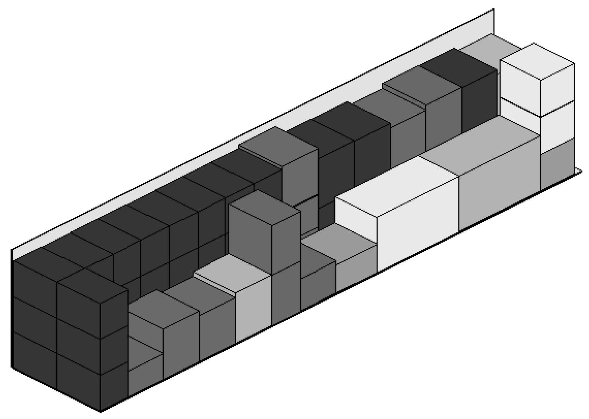
An example of container loading is presented in Figure 1. Some other requirements may appear in real-world applications, such as load bearing strength, weight distribution/limit, and cargo priority. See [2] for an extensive review on CLP constraints.

The CLP is strictly NP-Hard [3], and therefore, exact methods can effectively solve only small size instances. To deal with larger ones, heuristics are the current alternative. In a recent paper [4], CLP heuristics were categorized into three, not necessarily disjoint, groups:

• Conventional heuristics, which take advantage of the specific problem structure. A classical example is the wall-building procedure of George and Robinson [5], where the loading is made layer-by-layer across the depth of the container. Other examples of problem-dependent techniques applied to solve the CLP can be found in [6,7,8].
• Metaheuristics, which have been extensively applied to the CLP. Parreño et al. [9], for instance, conceived of a constructive procedure based on maximal-space representation. Insertion and deletion shifts directly affecting the container layout were used in a variable neighborhood search to improve partial solutions. Further studies include co-evolutionary computation techniques (e.g., Genetic Algorithms (GAs) [10,11]), trajectory-based methods (e.g., simulated annealing [12], the greedy randomized adaptive search procedure [13], and tabu search [14]), and swarm intelligence systems (e.g., bee colony algorithm [15]).
• Tree search methods, which have produced good-quality solutions to the CLP. Fanslau and Bortfeldt [4], for instance, proposed a tree search method that keeps a list of empty spaces to be filled by blocks of boxes. Similar contributions can be found in [16,17,18,19].

Despite this general classification, it has been proven to be pertinent to combine distinct optimization techniques to exploit their main advantages simultaneously (e.g., a metaheuristic with an Integer Linear Programming (ILP) solver), which has been referred to as hybrid metaheuristics [20,21]. Some authors prefer to refer to heuristic algorithms particularly made by the interoperation of metaheuristics and mathematic programming techniques as matheuristics [22]. In this paper, we propose a two-phase approach to tackle the CLP, motivated by a general idea of decomposing the CLP into two subproblems [11,23], namely a three-dimensional problem of generating blocks of boxes and a two-dimensional problem of loading blocks on the floor of the container. In our proposal, the three-dimensional problem is solved by means of constructive algorithms from the literature, and the two-dimensional problem is solved by means of a hybrid metaheuristic. Computational experiments performed on weakly-heterogeneous benchmark instances (with a few types of boxes) show that our approach competes with state-of-the-art CLP algorithms.

The remainder of this work is organized as follows. In Section 2, we describe our algorithm. In Section 3, we provide computational experiments on benchmark instances from the literature and present a discussion of the results. Finally, in Section 4, we close the paper with some conclusions and future perspectives.

2. Block-Loading Hybrid Metaheuristic

Our Block-Loading Hybrid Metaheuristic (BLHM) algorithm is segmented into two subsequent phases: block generation and block loading. On the one hand, the block generation phase is very fast and completely deterministic. Constructive algorithms from the literature [7] perform this task. On the other hand, the block loading phase is non-deterministic. It comprises the generate-and-solve methodology [24,25,26], a problem-independent hybrid optimization framework characterized by the interoperation of a metaheuristic with an ILP solver. In what follows, we describe how BLHM works to address the CLP.

2.1. Block Generation

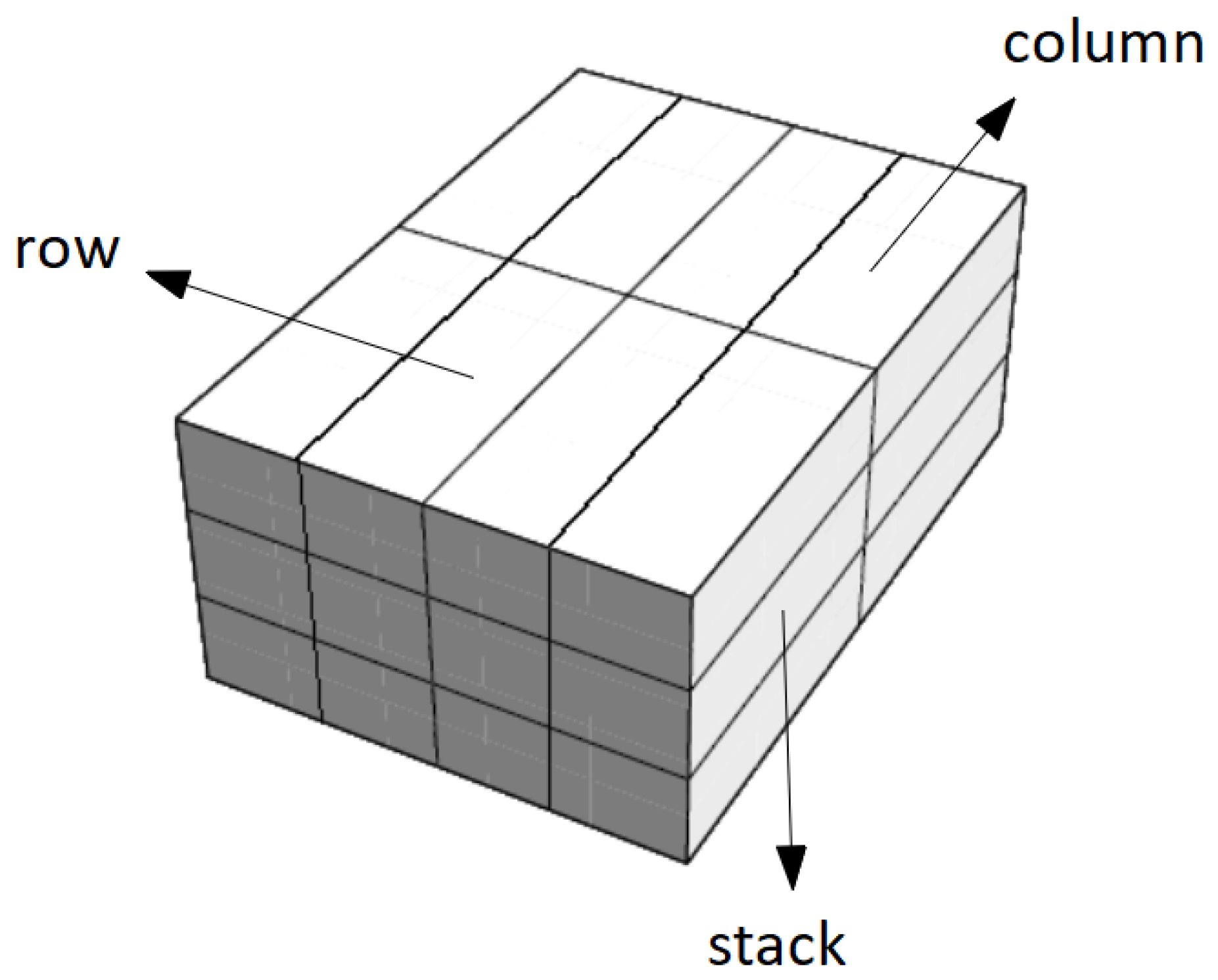
Some CLP algorithms [4,7,8] have received notoriety for loading cuboid blocks of boxes instead of single boxes, thus being properly classified as block-building approaches. By definition, a block is a set of boxes placed compactly inside its Minimum Bounding Cuboid (MBC) [7]. Existing research classifies blocks into two types: simple blocks and guillotine blocks. Simple blocks consist of identical boxes, in the same spatial orientation and occupying the total volume of their respective MBCs. A pseudocode [7] to generate simple blocks is presented in Algorithm 1, which roughly produces valid blocks with $n_x$ boxes in a row, $n_y$ boxes in a column, and $n_z$ boxes in a stack, all of them of the same type, as illustrated in Figure 2.

Algorithm 1 Generating simple blocks (adapted from the original paper [7]).

Input: A container with dimensions L, W, and H and a collection of boxes grouped into types. Each type t has a length $l_t$, a width $w_t$, a height $h_t$, and a quantity $q_t$ of boxes available to be loaded. Output: Set B of simple blocks. 1: $B\leftarrow \varnothing$ 2: for each box type t do 3:  for each allowed orientation of $(l_t,w_t,h_t)$ do 4:   for $n_x=1$ to $q_t$ do 5:    for $n_y=1$ to $\frac{q_t}{n_x}$ do 6:     for $n_z=1$ to $\frac{q_t}{n_x\times n_y}$ do 7:      if $n_x\times l_t\le L$ & $n_y\times w_t\le W$ & $n_z\times h_t\le H$ then 8:       Create a block b with dimensions $(n_x\times l_t,n_y\times w_t,n_z\times h_t)$, and add it to B 9: returnB

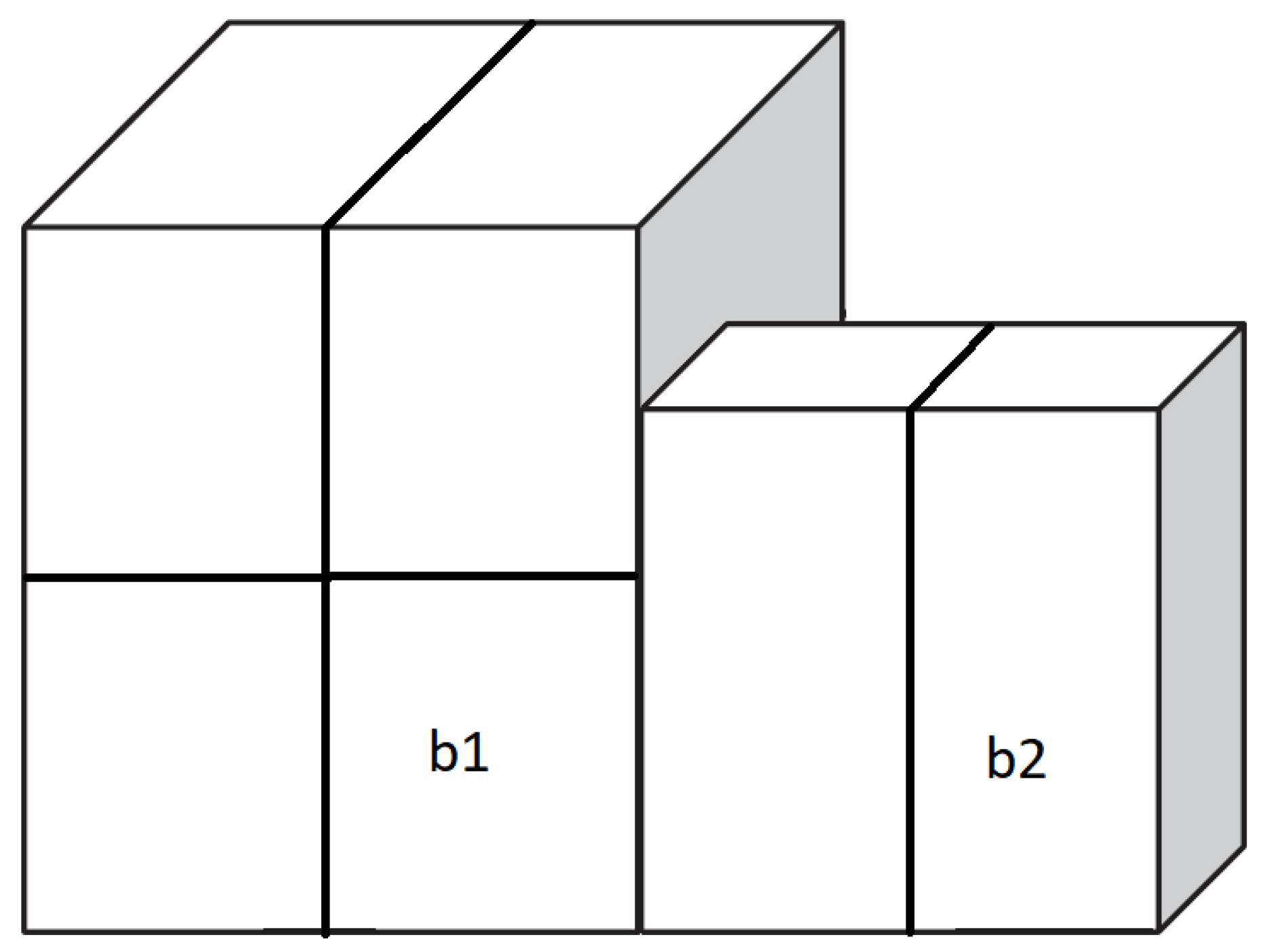
Conversely, guillotine blocks consist of multiple types of boxes possibly placed in different spatial orientations. A pseudocode to generate guillotine blocks, proposed by Zhu and Lim [7], is given in Algorithm 2. B, $PG$, and $NG$ denote, respectively, the set of blocks generated so far, the set of blocks generated in the previous iteration, and the set of blocks generated in the current generation. Given one block $b_1$ from B and another block $b_2$ from $PG$, guillotine blocks are generated by combining the two blocks along the length, width, or height direction of the container, as illustrated in Figure 3.

Algorithm 2 Generating guillotine blocks (adapted from the original paper [7]).

Input: Set B of simple blocks (see Algorithm 1). Output: Extended set B of guillotine blocks.   1: $PG\leftarrow B$   2: repeat   3:  $NG\leftarrow \varnothing$   4:  for each block $b_1$ in $PG$ do   5:   for each block $b_2$ in B do   6:    for each direction $dir$ in $\{L,W,H\}$ do   7:     Combine $b_1$ and $b_2$ along the direction $dir$ to obtain block b   8:     Add b to $NG$ if b is feasible and no equivalent block exists in B   9:  $B\leftarrow B\cup NG$ 10:  $PG\leftarrow NG$ 11: until$PG=\varnothing$ 12: returnB

Fully-Supported Blocks (FSBs) [7] are blocks complying with the stability constraint. They are generated handling an attribute called packing area, which is the rectangular region on the top face of the block that is fully covered by top faces of boxes belonging to its MBC. Obviously, simple blocks are FSBs. Guillotine FSBs are generated according to some rules. For instance, let $b_1$ and $b_2$ be two guillotine FSBs with packing area $p_1$ and $p_2$, respectively. Such blocks can be combined along the length (resp. width) direction if and only if they have the same height (i.e., $b_1.h=b_2.h$) and the sum of the lengths (resp. widths) of their packing areas spans the entire length (resp. width) of their MBCs, i.e., $p_1.l+p_2.l=b_1.l_1+b_2.l_2$ (resp. $p_1.w+p_2.w=b_1.w_1+b_2.w_2$). When $b_1$ and $b_2$ are combined along the length (resp. width) direction, the resultant packing area $p_3$ of the new FSB $b_3$ is given by $p_3.l=p_1.l+p_2.l$ (resp. $p_3.l=\min \{p_1.l,p_2.l\}$) and $p_3.w=\min \{p_1.w,p_2.w\}$ (resp. $p_3.w=p_1.w+p_2.w$). Another scenario arises when combining $b_1$ and $b_2$ along the height direction. One can place $b_1$ on the top face of block $b_2$ if and only if the base area of $b_1$ fits entirely into $p_2$. Then, the packing area of the resultant FSB $b_3$ is equivalent to $p_1$. See [4,7,27] for illustrations of the concepts related to blocks of boxes.

The first phase of our BLHM uses Algorithms 1 and 2 to generate FSBs. Let B be the set of FSBs obtained after running such algorithms. We now resort to an evaluation function to identify promising FSBs belonging to B. An FSB $b_i$, $1\le i\le |B|$, is assumed to be promising if and only if:

$$f\left(b_i\right)=\frac{v_i}{V_i}\ge MinUtil$$

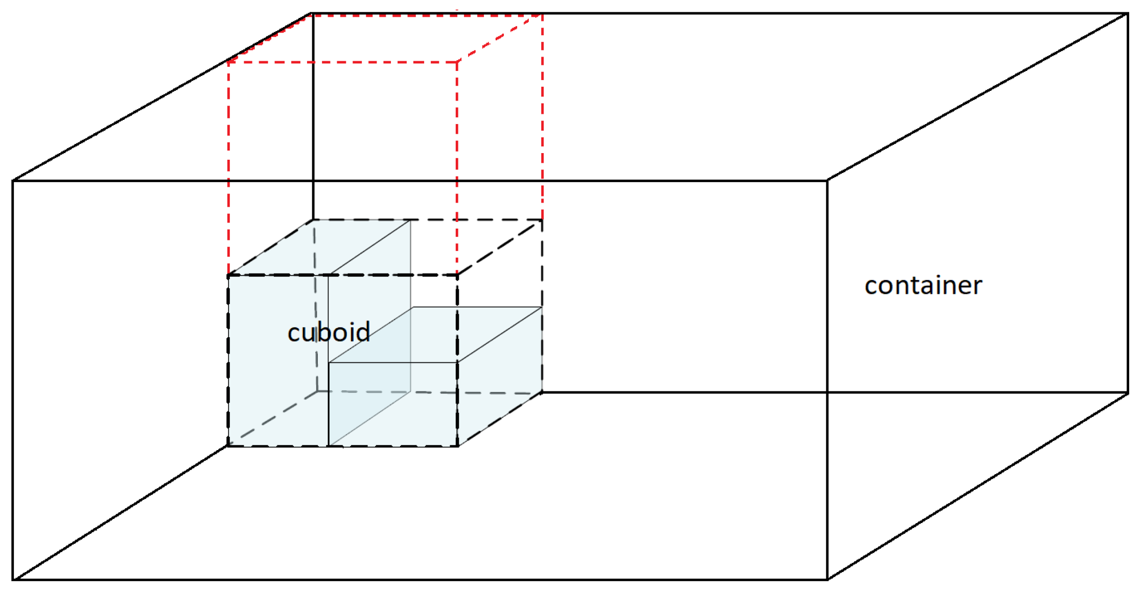
where $v_i$ is the volume of boxes in $b_i$; $V_i$ is the volume of the virtual space occupied by $b_i$, calculated as the product of the base area of its MBC by the height of the container (instead of the height of its MBC, since in the next phase, we just place FSBs on the floor of the container); and $MinUtil$ is a parameter in the real interval $[0,1]$. Note that when $MinUtil$ is near one, only promising FSBs with small residual spaces are considered to the next phase. In this way, we reject FSBs that present a considerable volume not occupied by boxes and FSBs that are too low in relation to the height of the container, as illustrated in Figure 4. In what follows, we refer to $\overline{B}\subset B$ as the set of promising FSBs.

2.2. Block Loading

In the second phase of our BLHM algorithm, we use the GS hybrid framework. In the sequence, we first present an ILP model to the problem of loading FSBs on the container floor and then propose an application of the GS framework to the problem.

2.2.1. ILP Model

Loading FSBs on the container floor is a two-dimensional C&P problem. We implement a well-known ILP model for orthogonal two-dimensional C&P problems [28]. Let $u_{ijk}$ be a binary decision variable standing for the decision of whether or not to load an FSB of type i at coordinate $(j,k)$ of the container floor.

$$u_{ijk}=\left\{\begin{array}{cc}1,\hfill & \mathrm{if} \mathrm{an} \mathrm{FSB} \mathrm{of} \mathrm{type} i \mathrm{is} \mathrm{placed} \mathrm{at}\hfill \\ & \mathrm{coordinate} (j,k),\hfill \\ 0,\hfill & \mathrm{otherwise}.\hfill \end{array}\right.$$

The elements j and k belong, respectively, to the following discretization sets:

$$X=\{x|x=\sum _{i=1}^{|\overline{B}|}{\alpha }_i{l}_i,x\le L-\underset{1\le i\le |\overline{B}|}{min}\{l_i\},{\alpha }_i\in {\mathbb{Z}}^{+}\}$$

$$Y=\{y|y=\sum _{i=1}^{|\overline{B}|}{\beta }_i{w}_i,y\le W-\underset{1\le i\le |\overline{B}|}{min}\{w_i\},{\beta }_i\in {\mathbb{Z}}^{+}\}$$

To avoid overlapping of FSBs, the incidence matrix $g_{ijkpq}$ is defined as:

$$g_{ijkpq}=\left\{\begin{array}{cc}1,\hfill & \mathrm{if} j\le p\le j+l_i-1\hfill \\ & \mathrm{and} k\le q\le k+w_i-1,\hfill \\ 0,\hfill & \mathrm{otherwise}.\hfill \end{array}\right.$$

which is computed a priori for each FSB of type i, for each coordinate $(j,k)$, and for each coordinate $(p,q)$. Finally, the ILP model is defined as follows:

$$\begin{array}{cc}\hfill max& \sum _{i=1}^{|\overline{B}|}\sum _{j\in X}\sum _{k\in Y}{v}_i{u}_{ijk}\hfill \end{array}$$

(1)

$$\begin{array}{cc}\hfill \mathrm{s}.\mathrm{t}.& \sum _{i=1}^{|\overline{B}|}\sum _{j\in X}\sum _{k\in Y}{g}_{ijkpq}{u}_{ijk}\le 1,\forall p\in X,\forall q\in Y\hfill \end{array}$$

(2)

$$\begin{array}{cc}\hfill & \sum _{i=1}^{|\overline{B}|}\sum _{j\in X}\sum _{k\in Y}{q}_i^t{u}_{ijk}\le q_t,t=1,\dots ,m\hfill \end{array}$$

(3)

$$\begin{array}{cc}\hfill & u_{ijk}\in \{0,1\},i=1,\dots ,|\overline{B}|,\forall j\in X,\forall k\in Y\hfill \end{array}$$

(4)

The objective function (1) maximizes the volume of loaded FSBs inside the container. Constraints (2) avoid overlapping of FSBs in any feasible solution. Let $q_i^t$ represent the quantity of boxes of type t in an FSB of type i. Constraints (3) impose that, for each box type t, the quantity of loaded boxes of this type must not exceed the number of boxes available. Finally, Constraints (4) specify the domain of variables. The ILP model (1)–(4) contains $O(|\overline{B}|\times |X|\times |Y|)$ variables and $O(|X|\times |Y|)$ constraints. Since the product $|X|\times |Y|$ may be too large for practical instances of this problem, the number of constraints and variables can easily reach the order of millions, which discourages the straightforward use of classical ILP techniques.

2.2.2. Generate-and-Solve

ILP solvers are very effective at coping with combinatorial optimization problems up to a certain problem-specific instance size. Recently, approaches based on problem instance reduction [29], such as generate-and-solve [24,25,30], construct, merge, solve and adapt [31], and column reduction methods [32], have shown that, when a problem instance is too large to be directly solved by an ILP solver, it might be possible to reduce the problem instance in a way such that it can be effectively solved by the ILP solver and it still contains high-quality solutions to the original problem instance.

The GS hybrid optimization framework has been introduced to cope with hard combinatorial optimization problems, such as those of the C&P family. The framework prescribes the integration of two distinct conceptual components: the Generator of Reduced Instances (GRI) and the Solver of Reduced Instances (SRI), as depicted in Figure 5.

An exact method (e.g., ILP solver) encapsulated in the SRI component is in charge of solving reduced instances (i.e., subproblems) of the original problem that still preserve its conceptual structure. Thus, a feasible solution to a given subproblem will also be a feasible solution to the original problem. At a higher level, a metaheuristic (e.g., GA) works on the complementary optimization problem of generating reduced instances, which, when submitted to the SRI, produce feasible solutions whose objective function values can be used as a figure of merit (fitness) of the associated subproblems, thus guiding the search process. The interaction between GRI and SRI proceeds until a given stopping condition is satisfied. The best solution obtained by the solver to any of the subproblems generated by the metaheuristic is deemed to be the final solution.

2.2.3. Random Key Genetic Algorithm

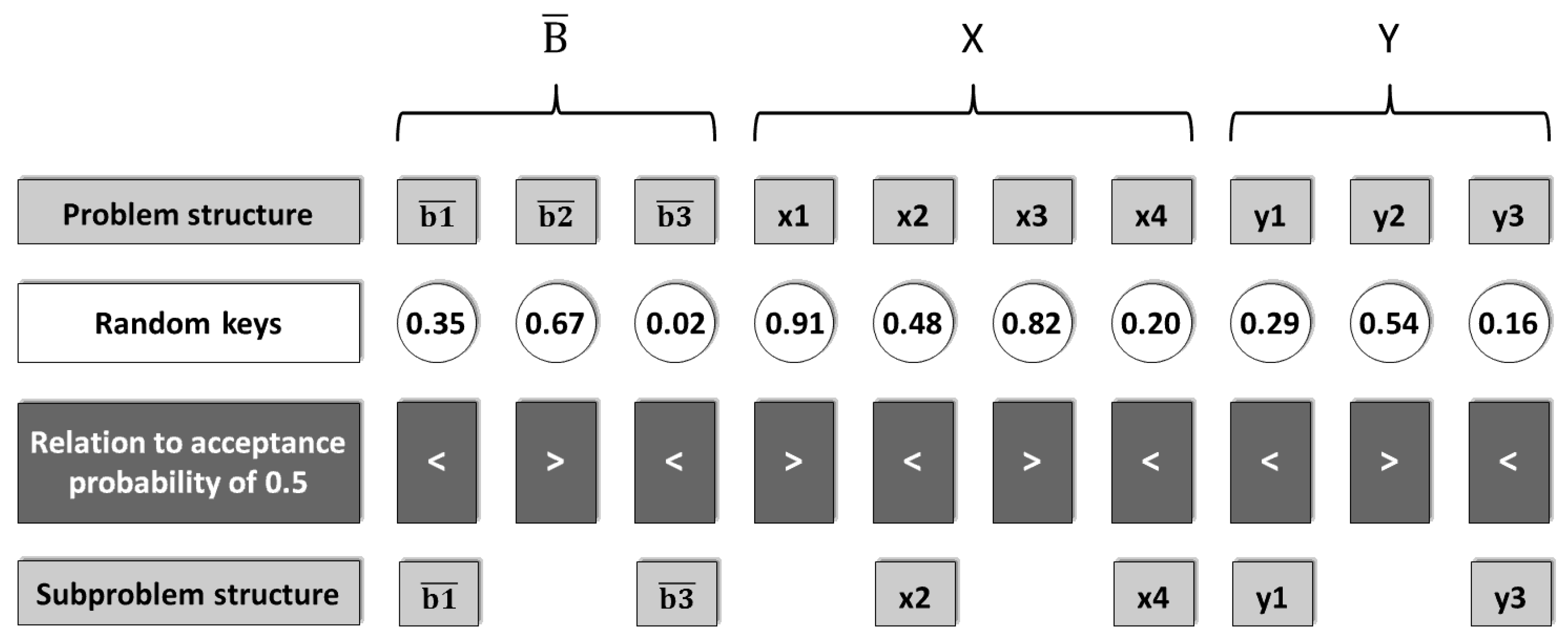
One can generate reduced instances of the block loading problem by removing some of the types of FSBs and/or some of the elements of the discretization sets from the ILP model (1)–(4). In our implementation, the GRI runs a Random Key Genetic Algorithm (RKGA) [33]. Individuals are represented by chromosomes (of random keys) with a size equal to $|\overline{B}|+|X|+|Y|$, as shown in Figure 6.

In this representation, each allele of the encoding scheme denotes the decision of counting (or not) on the presence of an element in the reduced instance. Let $p_{\overline{B}}$, $p_X$, and $p_Y$ be the probability of acceptance related to $\overline{B}$, X, and Y, respectively. If an allele $rk\left(\overline{b_i}\right)\le p_{\overline{B}}$, with $1\le i\le |\overline{B}|$, then the corresponding FSB will be a candidate FSB to be loaded on the container floor by the SRI. This insight is also applied to the discretization sets, i.e., if an allele $rk\left(x_j\right)\le p_X$, with $1\le j\le |X|$ (resp. $rk\left(y_k\right)\le p_Y$, with $1\le k\le |Y|$), then the corresponding element of X (resp. Y) will take part of the reduced instance. As an example in Figure 6, FSBs $\overline{b1}$ and $\overline{b3}$ take part in the subproblem to be solved by the SRI, since their alleles (or random keys) are less than the acceptance probability of 0.5. Regarding the discretization sets, elements $x2$, $x4$, $y1$, and $y3$ take part of the reduced instance. Therefore, $\overline{b1}$ and $\overline{b3}$ may be possibly loaded at coordinates $(x2,y1)$, $(x2,y3)$, $(x4,y1)$, and $(x4,y3)$.

The initial population contains p chromosomes, whose alleles are randomly generated in the real interval $[0,1]$. After an individual is translated to its ILP formulation and solved by means of an ILP solver, its fitness value is computed. Note that, if a chromosome includes all FSBs and coordinates, the original problem will be generated. However, it is very likely that the corresponding ILP model cannot be handled by the ILP solver. The population is then partitioned into two groups: a small group of $p_e$ elite individuals whose corresponding reduced instances present the best fitness values (i.e., objective function values) and the remaining set of $p-p_e$ non-elite individuals.

To evolve the population, a new generation must be produced. First, all elite individuals are carried over from generation g to generation $g+1$. Then, RKGA implements mutation by introducing $p_m$ mutants into the population. Mutants are vectors of random keys generated as elements of the initial population. Finally, discounting $p_e$ elite individuals and $p_m$ mutants, $p-p_e-p_m$ offspring individuals are produced through mating to complete p individuals that will make up the population of generation $g+1$. Mating (crossover) is performed as in [34]. Given two parents A and B randomly selected from the current population and a user-chosen probability $p_A>0.5$ that an offspring inherits the allele of A, for each allele $a=1,\dots ,n$ (where n is the number of genes), the child either takes the value of the $a^{\mathrm{th}}$ allele of A with probability $p_A$ or the corresponding allele of B with probability $1-p_A$.

3. Computational Experiments

Experiments were performed on a PC Intel Pentium i7, 8 × 3.60 GHz, 16 GB DDR3 RAM under Linux Ubuntu 14.05 LTS. We used CPLEX 12.7 and Java concert technology as underlying solver of the SRI. The time limit for each instance was set to 3600 seconds. The GRI ran an RKGA implemented in Java.

3.1. Control Parameters and Calibration

We conducted preliminary experiments to figure out the best input values for BLHM. To identify promising FSBs, we set $MinUtil=0.90$. Concerning the RKGA, we set $p=200$ individuals, $p_e=p_m=0.20\times p$, and $p_A=0.7$. To control the duration of the optimization process, the maximum number of generations was set to 400, while the total time to stop was set to 3600 seconds. If the best fitness value did not change in 15 consecutive generations, a new population consisting of the two best individuals and $p-2$ random ones was generated. The acceptance probabilities were set to $p_{\overline{B}}=\frac{L\times W}{min\{l_t\times w_t\}}\times \frac{1}{|\overline{B}|}$, $p_X=\frac{L}{min\{l_t\}}\times \frac{1}{|X|}$, and $p_Y=\frac{1}{|Y|}$, for $t=1,\dots ,m$. The CPLEX time limit of 60 seconds was set to solve each subproblem.

3.2. Numerical Results

To evaluate the potentialities behind our BLHM algorithm, computational experiments were performed over difficult benchmark instances proposed by Bischoff and Ratcliff [6], which can be accessed via OR-Library [35]. Instances can be either weakly heterogeneous (few types of boxes, each one with many units available) or strongly heterogeneous (many types of boxes, each one with few units available). We decided to conduct our analysis only on weakly-heterogeneous datasets BR1 and BR2, which contain three and five types of boxes, respectively, after preliminary tests showed that the required computation time would be considerably high to compete with alternative approaches for strongly-heterogeneous instances.

We present results in

Table 1. Results for group BR1.

Instance	CLTRS [4]	ID-GLTS [7]	BSG-VCS [36]	BLHM
				Avg	Best*
BR1-001	93.83	93.80	93.53	95.12	95.83 *
BR1-002	95.45	94.94	96.01	95.24	97.67 *
BR1-003	91.03	91.03	91.03	92.11	92.67 *
BR1-004	91.84	91.84	91.84	94.55	95.26 *
BR1-005	95.14	95.14	95.14	93.85	94.63
BR1-006	95.72	94.63	96.02	93.20	93.49
BR1-007	94.14	93.57	94.03	93.74	94.60 *
BR1-008	97.05	97.05	97.18	93.88	94.53
BR1-009	91.57	90.62	91.87	87.61	87.61
BR1-010	94.81	94.67	94.81	93.10	93.20
BR1-011	91.49	91.84	92.54	90.37	91.11
BR1-012	94.08	93.67	93.67	91.45	91.95
BR1-013	97.14	97.43	97.60	95.34	95.58
BR1-014	94.37	94.63	94.70	91.30	91.68
BR1-015	95.38	96.74	96.96	92.84	93.29
BR1-016	95.75	95.55	96.20	93.14	94.21
BR1-017	97.80	97.29	97.97	96.21	96.40
BR1-018	88.49	88.49	88.49	88.95	89.57 *
BR1-019	94.73	94.73	95.13	94.40	94.81
BR1-020	94.20	95.23	94.30	91.53	92.46
BR1-021	94.69	93.77	94.69	93.47	93.48
BR1-022	95.34	94.46	94.73	92.58	93.89
BR1-023	94.15	94.67	94.69	96.53	96.54 *
BR1-024	90.75	91.18	91.42	91.51	91.63 *
BR1-025	94.83	95.25	95.17	93.27	94.26
BR1-026	93.81	93.81	93.81	93.17	93.67
BR1-027	91.67	91.95	92.54	93.60	93.60 *
BR1-028	93.84	93.46	94.73	91.46	92.53
BR1-029	93.95	93.92	94.45	93.52	94.45 *
BR1-030	97.54	97.13	98.09	94.43	95.08
BR1-031	95.54	94.65	95.67	92.84	93.32
BR1-032	97.01	97.01	97.01	94.84	95.07
BR1-033	97.63	97.55	97.75	94.17	94.88
BR1-034	94.62	94.62	95.47	92.66	92.87
BR1-035	93.60	94.05	94.14	91.74	92.30
BR1-036	95.47	95.36	94.68	94.05	94.51
BR1-037	95.16	94.97	95.42	92.65	93.16
BR1-038	90.64	90.11	90.71	90.92	91.30 *
BR1-039	96.40	96.48	96.48	94.07	94.19
BR1-040	94.52	93.96	93.98	92.96	93.53
BR1-041	94.55	94.97	95.39	93.89	94.55
BR1-042	94.24	94.86	95.29	93.47	94.37
BR1-043	95.61	95.75	96.18	83.98	86.02
BR1-044	87.97	88.21	88.21	83.97	84.03
BR1-045	96.38	96.23	96.38	93.76	94.12
BR1-046	94.13	94.13	94.13	90.80	91.27
BR1-047	95.39	96.16	96.29	92.83	93.56
BR1-048	95.95	95.45	95.45	94.93	95.65
BR1-049	95.03	94.29	94.77	92.61	94.10
BR1-050	97.55	97.76	98.16	94.45	95.56

* The best solution of BLHM over 10 runs is better than the solutions found by the other algorithms.

and

Table 2. Results for group BR1 (cont.).

Instance	CLTRS [4]	ID-GLTS [7]	BSG-VCS [36]	BLHM
				Avg	Best*
BR1-051	97.11	97.11	97.08	95.12	95.87
BR1-052	94.73	94.60	94.73	95.78	95.81 *
BR1-053	89.59	89.59	91.65	93.03	93.70 *
BR1-054	92.37	92.54	93.05	93.05	93.33 *
BR1-055	90.62	90.62	90.62	87.64	87.64
BR1-056	97.26	96.14	97.32	95.71	96.68
BR1-057	95.60	95.48	96.22	94.24	95.49
BR1-058	94.45	92.61	93.94	94.17	94.68 *
BR1-059	97.57	96.76	96.38	95.99	97.16
BR1-060	95.86	95.86	95.96	93.61	94.88
BR1-061	95.90	95.90	95.97	91.67	93.69
BR1-062	93.07	92.96	94.20	92.16	92.76
BR1-063	91.76	93.15	93.05	92.30	93.66 *
BR1-064	94.59	94.24	95.44	91.49	91.83
BR1-065	97.71	97.87	97.87	95.63	96.78
BR1-066	96.16	95.39	96.20	94.92	95.81
BR1-067	95.92	95.72	96.06	92.96	93.50
BR1-068	97.06	96.81	97.06	94.82	95.23
BR1-069	92.93	91.37	92.38	91.48	92.65
BR1-070	91.35	91.35	90.71	94.94	95.19 *
BR1-071	92.98	91.97	93.14	93.36	93.57 *
BR1-072	92.43	92.72	92.52	93.12	93.60 *
BR1-073	91.71	91.67	91.66	93.53	94.52 *
BR1-074	94.43	94.68	94.98	91.33	92.57
BR1-075	93.66	94.55	94.55	93.13	93.13
BR1-076	96.56	96.59	96.67	95.47	96.30
BR1-077	97.26	97.26	97.26	93.80	94.84
BR1-078	93.84	93.95	94.67	93.22	93.29
BR1-079	94.82	94.82	94.82	94.88	95.40 *
BR1-080	95.91	96.36	96.65	95.11	95.11
BR1-081	92.77	92.44	92.44	91.16	92.30
BR1-082	93.74	93.83	94.39	91.75	93.17
BR1-083	95.83	95.83	95.83	92.72	94.57
BR1-084	93.84	94.15	94.40	93.47	94.51 *
BR1-085	97.99	97.55	98.03	95.50	95.80
BR1-086	96.14	95.11	95.11	94.15	94.81
BR1-087	93.76	93.38	93.76	89.49	91.12
BR1-088	94.29	93.19	94.54	90.20	91.40
BR1-089	88.21	88.21	88.21	93.17	94.24 *
BR1-090	92.82	92.52	92.82	88.96	89.46
BR1-091	97.09	97.14	97.14	95.17	95.52
BR1-092	93.10	90.88	92.71	92.80	93.27 *
BR1-093	95.91	95.90	95.67	93.12	94.17
BR1-094	95.44	95.97	95.97	93.39	95.08
BR1-095	95.20	95.92	95.70	92.90	92.90
BR1-096	95.79	95.79	95.79	93.28	94.22
BR1-097	94.87	93.78	94.87	93.90	94.41
BR1-098	96.14	96.69	96.69	93.96	94.87
BR1-099	93.82	94.16	94.48	89.16	90.39
BR1-100	96.62	98.16	98.16	94.04	94.68

* The best solution of BLHM over 10 runs is better than the solutions found by the other algorithms.

(BR1) and

Table 3. Results for group BR2.

Instance	CLTRS [4]	ID-GLTS [7]	BSG-VCS [36]	BLHM
				Avg	Best*
BR2-001	95.50	95.55	95.98	91.85	92.71
BR2-002	95.50	95.22	95.11	93.40	93.74
BR2-003	94.14	95.52	95.42	89.91	91.63
BR2-004	93.68	93.39	94.23	93.91	95.16 *
BR2-005	95.89	96.24	96.24	92.13	93.77
BR2-006	96.33	96.24	96.65	91.40	93.27
BR2-007	96.19	95.70	96.70	93.13	94.18
BR2-008	94.12	94.14	94.20	91.39	91.63
BR2-009	95.23	94.39	95.00	91.34	92.12
BR2-010	96.69	96.15	96.33	94.30	95.25
BR2-011	93.34	94.02	95.21	90.24	91.69
BR2-012	93.75	94.56	94.85	91.12	92.00
BR2-013	95.75	96.58	96.71	92.88	94.64
BR2-014	94.11	94.18	94.60	92.67	93.88
BR2-015	95.85	96.00	96.16	91.80	93.68
BR2-016	94.21	94.88	95.79	92.47	93.05
BR2-017	96.07	95.88	95.93	91.68	92.85
BR2-018	92.74	93.49	94.70	90.37	91.44
BR2-019	95.07	95.73	95.60	91.94	93.55
BR2-020	94.36	94.77	94.42	91.92	93.48
BR2-021	93.36	93.68	95.41	91.87	93.05
BR2-022	93.76	93.98	94.81	90.23	91.32
BR2-023	91.01	90.43	90.98	92.48	92.68 *
BR2-024	92.28	92.46	92.55	91.13	92.34
BR2-025	95.60	95.24	96.34	91.87	92.86
BR2-026	95.19	95.09	95.38	92.55	93.73
BR2-027	93.34	93.24	93.95	92.31	92.90
BR2-028	93.74	93.82	94.52	91.85	93.17
BR2-029	96.67	96.04	97.02	96.62	97.02 *
BR2-030	97.33	97.59	97.94	94.22	94.35
BR2-031	95.75	94.74	96.28	90.66	92.26
BR2-032	95.72	95.61	96.45	92.63	93.39
BR2-033	96.04	96.14	95.87	93.95	94.31
BR2-034	95.83	95.10	95.43	92.78	93.86
BR2-035	95.46	95.76	95.74	91.98	92.41
BR2-036	95.27	95.47	95.29	93.92	94.44
BR2-037	94.45	94.41	95.79	92.14	93.32
BR2-038	93.82	94.67	94.67	90.45	91.16
BR2-039	95.79	96.64	97.25	94.75	95.47
BR2-040	93.06	93.31	94.07	91.05	92.19
BR2-041	94.14	94.14	93.83	93.01	93.45
BR2-042	95.20	95.10	95.56	92.88	94.06
BR2-043	94.00	94.44	94.44	90.33	90.77
BR2-044	90.14	90.70	92.33	89.38	89.38
BR2-045	95.10	95.43	95.59	92.76	93.84
BR2-046	93.61	93.67	94.12	93.07	93.57
BR2-047	95.76	95.96	96.03	93.51	93.88
BR2-048	96.18	96.87	97.35	94.06	94.94
BR2-049	95.99	95.94	96.03	94.35	94.41
BR2-050	97.03	97.04	97.58	93.85	94.68

* The best solution of BLHM over 10 runs is better than the solutions found by the other algorithms.

and

Table 4. Results for group BR2 (cont.).

Instance	CLTRS [4]	ID-GLTS [7]	BSG-VCS [36]	BLHM
				Avg	Best*
BR2-051	96.47	96.17	96.56	94.37	95.11
BR2-052	95.30	95.76	95.31	93.89	94.31
BR2-053	92.27	93.18	94.06	93.71	94.06 *
BR2-054	94.38	94.90	95.31	90.77	91.81
BR2-055	93.03	93.60	94.33	90.92	91.55
BR2-056	96.26	96.26	96.84	93.05	93.87
BR2-057	96.46	96.41	97.14	92.09	93.28
BR2-058	94.97	94.11	94.97	93.86	94.58
BR2-059	96.63	97.13	96.72	94.60	95.86
BR2-060	95.64	94.62	95.64	92.03	92.35
BR2-061	93.03	94.80	94.80	90.51	91.77
BR2-062	95.81	95.77	96.15	90.74	91.31
BR2-063	93.80	92.84	93.54	91.43	92.99
BR2-064	94.74	93.11	93.60	91.71	92.17
BR2-065	94.78	95.39	96.17	93.90	94.00
BR2-066	95.07	95.61	96.62	92.88	93.70
BR2-067	96.04	95.67	96.84	92.41	93.50
BR2-068	93.78	93.78	95.06	93.35	93.78
BR2-069	91.13	91.72	92.34	92.50	93.01 *
BR2-070	93.24	92.21	94.32	91.76	92.75
BR2-071	95.17	95.37	96.04	93.71	94.71
BR2-072	92.12	92.82	93.31	91.56	92.72
BR2-073	93.42	93.25	94.44	92.57	93.68
BR2-074	94.03	94.18	95.31	91.22	92.53
BR2-075	94.87	95.16	95.47	92.60	93.71
BR2-076	96.64	96.00	97.05	94.38	95.58
BR2-077	95.18	96.13	96.58	94.25	95.04
BR2-078	95.22	95.17	95.94	92.69	93.78
BR2-079	96.46	96.24	96.98	94.14	94.53
BR2-080	93.33	94.10	94.34	92.82	93.99
BR2-081	92.68	93.70	93.67	92.72	93.28
BR2-082	94.50	94.41	95.11	91.96	92.80
BR2-083	96.45	95.83	96.61	93.11	93.87
BR2-084	92.77	92.27	93.26	92.82	93.98 *
BR2-085	96.85	96.90	97.24	95.21	95.61
BR2-086	94.75	95.29	95.83	93.13	94.27
BR2-087	93.76	94.23	94.84	90.57	91.18
BR2-088	92.34	92.99	93.64	92.12	93.62
BR2-089	89.58	89.96	90.57	92.58	93.04 *
BR2-090	94.55	95.04	95.04	91.68	92.17
BR2-091	94.53	95.16	95.64	92.89	94.10
BR2-092	93.96	93.79	94.30	91.80	92.25
BR2-093	95.35	95.35	95.35	93.38	94.88
BR2-094	97.11	96.66	97.42	93.75	94.36
BR2-095	94.98	95.84	95.85	94.00	94.00
BR2-096	96.83	97.04	98.27	92.56	93.27
BR2-097	95.53	94.64	95.01	92.78	93.92
BR2-098	96.38	96.58	97.31	92.92	93.74
BR2-099	96.84	96.83	97.33	93.56	95.08
BR2-100	95.17	95.66	95.57	91.51	95.23

* The best solution of BLHM over 10 runs is better than the solutions found by the other algorithms.

(BR2). In these tables, for each instance, we present the volume utilization achieved by well-known state-of-the-art approaches enforcing orientation and stability constraints: the Container Loading by TRee Search (CLTRS) of Fanslau and Bortfeldt [4], the Iterative-Doubling-Greedy Lookahead Tree Search (ID-GLTS) of Zhu and Lim [7], and the Beam Search (BSG-VCS) of Araya, Guerrero, and Nuñes [36] with a new heuristic function for selecting boxes. To the best of our knowledge, BSG-VCS has reported the best results to date. It is important to stress that CLTRS, ID-GLTS, and BSG-VCS have a maximum runtime of 500 s for each instance. The columns related to BLHM show, for each instance, the average (avg.) and the best (best) solution values found by our algorithm over 10 runs. We indicate by bold font the best solution found among the four CLP algorithms. To compare the algorithms, since BLHM is non-deterministic, we consider its average value (and denote by * in the case that the best solution of BLHM is better than the solutions found by the other algorithms).

We begin the discussions on experimental analysis by stating that there is not a particular algorithm that stands out from the others for all instances. Taking as the reference group BR1, for instance, BLHM found new best solutions for 24 (out of 100) instances. The average solution obtained by CLTRS, ID-GLTS, BSG-VCS, and BLHM was 94.51, 94.40, 94.74, and 92.97 (considering the average column), respectively. For BR1-043, the result of 83.98 obtained by BLHM was very small when compared to the best one, namely 96.18. We believe this is due to the small number of FSBs generated in the first phase of BLHM.

Concerning group BR2, BLHM obtained the best solutions for seven (out of 100) instances. The average solution of CLTRS, ID-GLTS, BSG-VCS, and BLHM was 94.73, 94.85, 95.38, and 92.52 (considering the average column), respectively. It is important to note that the efficiency of BLHM decreased as the heterogeneity of the instances increased.

4. Conclusions

In this work, we presented a two-phase approach to tackle the container loading problem. The idea behind our algorithm is to decompose the CLP into two subproblems, namely a three-dimensional problem of generating a set of blocks of boxes and a two-dimensional problem of loading a subset of blocks on the container floor. Constructive algorithms conducted the former task, while the generate-and-solve hybrid framework dealt with the latter one. Computational experiments performed on weakly-heterogeneous datasets showed that our algorithm found new best solutions for 31 (out of 200) instances of groups BR1 and BR2. Its performance however deteriorated as the number of types of boxes increases. As future work, we intend to explore other CLP constraints, e.g., load bearing strength and weight distribution, and to investigate other strategies to compare eventually our results to methods more advantageous in solving strongly-heterogeneous problems [37]. Future studies might cover solving the multi-container loading problem [38] and ship loading problem [39] by modifying our suggested method. Another perspective is to study the application of the GS hybrid framework to classical combinatorial optimization problems.

References

- Wäscher, G.; Haußner, H.; Schumann, H. An improved typology of cutting and packing problems. Eur. J. Oper. Res. 2007, 183, 1109–1130. [Google Scholar] [CrossRef]
- Bortfeldt, A.; Wäscher, G. Constraints in container loading—A state-of-the-art review. Eur. J. Oper. Res. 2013, 229, 1–20. [Google Scholar] [CrossRef]
- Scheithauer, G. Algorithms for the container loading problem. In Operations Research Proceedings 1991; Springer: Berlin, Germany, 1992; pp. 445–452. [Google Scholar]
- Fanslau, T.; Bortfeldt, A. A tree search algorithm for solving the container loading problem. INFORMS J. Comput. 2010, 22, 222–235. [Google Scholar] [CrossRef]
- George, J.A.; Robinson, D.F. A heuristic for packing boxes into a container. Comput. Oper. Res. 1980, 7, 147–156. [Google Scholar] [CrossRef]
- Bischoff, E.E.; Ratcliff, M. Issues in the development of approaches to container loading. Omega 1995, 23, 377–390. [Google Scholar] [CrossRef] [Green Version]
- Zhu, W.; Lim, A. A new iterative-doubling Greedy–Lookahead algorithm for the single container loading problem. Eur. J. Oper. Res. 2012, 222, 408–417. [Google Scholar] [CrossRef]
- Araya, I.; Riff, M.C. A beam search approach to the container loading problem. Comput. Oper. Res. 2014, 43, 100–107. [Google Scholar] [CrossRef]
- Parreño, F.; Alvarez-Valdés, R.; Oliveira, J.; Tamarit, J.M. Neighborhood structures for the container loading problem: A VNS implementation. J. Heuristics 2010, 16, 1–22. [Google Scholar] [CrossRef]
- Gonçalves, J.F.; Resende, M.G. A parallel multi-population biased random-key genetic algorithm for a container loading problem. Comput. Oper. Res. 2012, 39, 179–190. [Google Scholar] [CrossRef]
- Gehring, H.; Bortfeldt, A. A genetic algorithm for solving the container loading problem. Int. Trans. Oper. Res. 1997, 4, 401–418. [Google Scholar] [CrossRef]
- Mack, D.; Bortfeldt, A.; Gehring, H. A parallel hybrid local search algorithm for the container loading problem. Int. Trans. Oper. Res. 2004, 11, 511–533. [Google Scholar] [CrossRef]
- Moura, A.; Oliveira, J.F. A GRASP approach to the container-loading problem. IEEE Intell. Syst. 2005, 20, 50–57. [Google Scholar] [CrossRef]
- Liu, J.; Yue, Y.; Dong, Z.; Maple, C.; Keech, M. A novel hybrid tabu search approach to container loading. Comput. Oper. Res. 2011, 38, 797–807. [Google Scholar] [CrossRef]
- Dereli, T.; Das, G.S. A hybrid ‘bee(s) algorithm’ for solving container loading problems. Appl. Soft Comput. 2011, 11, 2854–2862. [Google Scholar] [CrossRef]
- Morabito, R.; Arenales, M. An AND/OR-graph approach to the container loading problem. Int. Trans. Oper. Res. 1994, 1, 59–73. [Google Scholar] [CrossRef]
- Eley, M. Solving container loading problems by block arrangement. Eur. J. Oper. Res. 2002, 141, 393–409. [Google Scholar] [CrossRef]
- Pisinger, D. Heuristics for the container loading problem. Eur. J. Oper. Res. 2002, 141, 382–392. [Google Scholar] [CrossRef] [Green Version]
- He, K.; Huang, W. An efficient placement heuristic for three-dimensional rectangular packing. Comput. Oper. Res. 2011, 38, 227–233. [Google Scholar] [CrossRef]
- Raidl, G.R. Decomposition based hybrid metaheuristics. Eur. J. Oper. Res. 2015, 244, 66–76. [Google Scholar] [CrossRef]
- Blum, C.; Raidl, G.R. Hybrid Metaheuristics: Powerful Tools for Optimization; Springer: Berlin, Germany, 2016. [Google Scholar]
- Boschetti, M.; Maniezzo, V.; Roffilli, M.; Bolufé Röhler, A. Matheuristics: Optimization, Simulation and Control. In Hybrid Metaheuristics; Blesa, M., Blum, C., Di Gaspero, L., Roli, A., Sampels, M., Schaerf, A., Eds.; Lecture Notes in Computer Science; Springer: Berlin, Germany, 2009; Volume 5818, pp. 171–177. [Google Scholar]
- Haessler, R.W.; Brian Talbot, F. Load planning for shipments of low density products. Eur. J. Oper. Res. 1990, 44, 289–299. [Google Scholar] [CrossRef]
- Nepomuceno, N.; Pinheiro, P.; Coelho, A.L. Tackling the Container Loading Problem: A Hybrid Approach Based on Integer Linear Programming and Genetic Algorithms. In Evolutionary Computation in Combinatorial Optimization; Cotta, C., van Hemert, J., Eds.; Lecture Notes in Computer Science; Springer: Berlin, Germany, 2007; Volume Voume 4446, pp. 154–165. [Google Scholar]
- Nepomuceno, N.; Pinheiro, P.; Coelho, A.L. A Hybrid Optimization Framework for Cutting and Packing Problems. In Recent Advances in Evolutionary Computation for Combinatorial Optimization; Cotta, C., van Hemert, J., Eds.; Studies in Computational Intelligence; Springer: Berlin, Germany, 2008; Volume 153, pp. 87–99. [Google Scholar]
- Saraiva, R.; Nepomuceno, N.; Pinheiro, P. The Generate-and-Solve Framework Revisited: Generating by Simulated Annealing. In Evolutionary Computation in Combinatorial Optimization; Middendorf, M., Blum, C., Eds.; Lecture Notes in Computer Science; Springer: Berlin, Germany, 2013; Volume 7832, pp. 262–273. [Google Scholar]
- Wang, N.; Lim, A.; Zhu, W. A multi-round partial beam search approach for the single container loading problem with shipment priority. Int. J. Prod. Econ. 2013, 145, 531–540. [Google Scholar] [CrossRef]
- Beasley, J. An exact two-dimensional non-guillotine cutting tree search procedure. Oper. Res. 1985, 33, 49–64. [Google Scholar] [CrossRef]
- Blum, C.; Raidl, G.R. Hybridization Based on Problem Instance Reduction. In Hybrid Metaheuristics: Powerful Tools for Optimization; Springer: Cham, Switzerland, 2016; pp. 45–62. [Google Scholar] [CrossRef]
- Pinheiro, P.R.; Coelho, A.L.V.; de Aguiar, A.B.; Bonates, T.O. On the concept of density control and its application to a hybrid optimization framework: Investigation into cutting problems. Comput. Ind. Eng. 2011, 61, 463–472. [Google Scholar] [CrossRef]
- Blum, C.; Pinacho, P.; López-Ibáñez, M.; Lozano, J.A. Construct, Merge, Solve & Adapt: A new general algorithm for combinatorial optimization. Comput. Oper. Res. 2016, 68, 75–88. [Google Scholar] [CrossRef]
- Çağatay Iris; Pacino, D.; Ropke, S.; Larsen, A. Integrated Berth Allocation and Quay Crane Assignment Problem: Set partitioning models and computational results. Transp. Res. Part E Logist. Transp. Rev. 2015, 81, 75–97. [Google Scholar] [CrossRef] [Green Version]
- Bean, J.C. Genetic algorithms and random keys for sequencing and optimization. ORSA J. Comput. 1994, 6, 154–160. [Google Scholar] [CrossRef]
- Spears, W.M.; De Jong, K.A. On the virtues of parameterized uniform crossover. In Proceedings of the Fourth International Conference on Genetic Algorithms, San Diego, CA, USA, 13–16 July 1991; pp. 230–236. [Google Scholar]
- Beasley, J.E. OR-Library: Distributing test problems by electronic mail. J. Oper. Res. Soc. 1990, 1069–1072. [Google Scholar] [CrossRef]
- Araya, I.; Guerrero, K.; Nuñez, E. VCS: A new heuristic function for selecting boxes in the single container loading problem. Comput. Oper. Res. 2017, 82, 27–35. [Google Scholar] [CrossRef]
- Liu, S.; Tan, W.; Xu, Z.; Liu, X. A tree search algorithm for the container loading problem. Comput. Ind. Eng. 2014, 75, 20–30. [Google Scholar] [CrossRef]
- Tian, T.; Zhu, W.; Lim, A.; Wei, L. The multiple container loading problem with preference. Eur. J. Oper. Res. 2016, 248, 84–94. [Google Scholar] [CrossRef]
- Çağatay, I.; Christensen, J.; Pacino, D.; Ropke, S. Flexible ship loading problem with transfer vehicle assignment and scheduling. Transp. Res. Part B Methodol. 2018, 111, 113–134. [Google Scholar] [CrossRef]
Figure 1.
A container loading pattern with orientation and stability constraints.
Figure 2.
A simple block with four boxes in a row, two boxes in a column, and three boxes in a stack.
Figure 3.
A guillotine block obtained from the combination of two simple blocks.
Figure 4.
A representation of a guillotine block, its MBC, and the residual space on top of it.
Figure 5.
The generate-and-solve hybrid framework.
Figure 6.
Chromosome of random keys.