Tree Compatibility, Incomplete Directed Perfect Phylogeny, and Dynamic Graph Connectivity: An Experimental Study

Abstract

We study two problems in computational phylogenetics. The first is tree compatibility. The input is a collection $\mathcal{P}$ of phylogenetic trees over different partially-overlapping sets of species. The goal is to find a single phylogenetic tree that displays all the evolutionary relationships implied by $\mathcal{P}$. The second problem is incomplete directed perfect phylogeny (IDPP). The input is a data matrix describing a collection of species by a set of characters, where some of the information is missing. The question is whether there exists a way to fill in the missing information so that the resulting matrix can be explained by a phylogenetic tree satisfying certain conditions. We explain the connection between tree compatibility and IDPP and show that a recent tree compatibility algorithm is effectively a generalization of an earlier IDPP algorithm. Both algorithms rely heavily on maintaining the connected components of a graph under a sequence of edge and vertex deletions, for which they use the dynamic connectivity data structure of Holm et al., known as HDT. We present a computational study of algorithms for tree compatibility and IDPP. We show experimentally that substituting HDT by a much simpler data structure—essentially, a single-level version of HDT—improves the performance of both of these algorithm in practice. We give partial empirical and theoretical justifications for this observation.

1. Introduction

A phylogenetic tree is a graphical depiction of the evolutionary history of a collection of taxa (typically species or genes). The leaves are in one-to-one correspondence with the taxa, the internal nodes correspond to hypothetical ancestral taxa, while edges represent ancestor-descendant relationships. Here, we consider two problems in computational phylogenetics.

• The input to the tree compatibility problem is a collection $\mathcal{P}=\{{\mathcal{T}}_1,\dots ,{\mathcal{T}}_k\}$ of rooted phylogenetic trees with partially-overlapping taxon sets. $\mathcal{P}$ and the trees within it are called, respectively, a profile and the input trees. The problem is to find a tree $\mathcal{T}$ whose taxon set is the union of the taxon sets of the input trees, such that each input tree ${\mathcal{T}}_i$ can be obtained from the restriction of $\mathcal{T}$ to the leaf set of ${\mathcal{T}}_i$ through edge contraction. If such a tree $\mathcal{T}$ exists, then $\mathcal{P}$ is said to be compatible; otherwise, $\mathcal{P}$ is incompatible.
• The input to the incomplete directed perfect phylogeny problem (IDPP) is an $n\times k$ character matrix $A=\left[a_{ij}\right]$, where each row corresponds to a taxon and each column to a character. The state $a_{ij}$ of taxon i on character j is zero, one, or ?, depending on whether, for species i, character j is absent, present, or the state is unknown. A completion of A is a matrix obtained from A by replacing each ? by either zero or one. IDPP asks if A has a completion B with the following property. There exists a phylogenetic tree that explains the evolution of the taxa described by B with at most one $0\to 1$ state transition on each character.

It is well known that testing the compatibility of a collection of unrooted trees—an NP-complete problem [1]—is equivalent to the undirected version of IDPP, namely the problem of testing the compatibility of a collection of “partial binary characters” (bipartitions of a subset of a set of species) [2]. Since a profile of rooted trees is effectively a collection of unrooted trees that have a common root taxon, the preceding observation establishes the connection between rooted tree compatibility and IDPP. We should also note that a reduction from rooted tree compatibility to IDPP is implicit in the work of Chimani et al. [3].

Here, for completeness, we provide a short and direct proof of the equivalence of tree compatibility and IDPP. We go further and argue that a previous algorithm for IDPP is effectively a variation of a recent tree compatibility algorithm. We then present a computational study of algorithms for these problems. This study provides an opportunity to analyze the engineering issues that arise when applying dynamic graph connectivity data structures in a highly-specific context. Our empirical results show that, in this setting, simple data structures perform better than more sophisticated ones with better asymptotic bounds.

1.1. Background

Tree compatibility testing arises in supertree construction [4,5,6,7], where the goal is to assemble a comprehensive phylogenetic tree out of smaller trees for restricted sets of taxa. The tree compatibility problem, however, has wider uses. In fact, the first polynomial-time algorithm for testing tree compatibility, the Build algorithm of Aho et al. [8], was designed to solve a problem in relational databases, not phylogenetics. The connection with phylogenetics was noted later [1].

A recent algorithm, called $\mathtt{BuildNT}$ [9,10], solves the tree compatibility problem for an arbitrary profile $\mathcal{P}$ in $\mathcal{O}\left(M_{\mathcal{P}}{log}^2{M}_{\mathcal{P}}\right)$ time, where $M_{\mathcal{P}}$ denotes the total size of the trees in $\mathcal{P}$. $\mathtt{BuildNT}$ is closely related to Semple and Steel’s version of Build [2] (the suffix “NT” refers to the fact that the algorithm can be extended to profiles of trees with “nested taxa”; i.e., where internal nodes are labeled with higher order species [10]). There is one important difference between the two algorithms. Build relies on the triple graph, whose nodes are the species and where there is an edge between two species a and b if they are involved in a rooted triple in some input tree; that is, if there is a third species c such that, for some input tree, the lowest common ancestor of a and b is a descendant of the lowest common ancestor of a, b, and c. In contrast, $\mathtt{BuildNT}$ relies on the display graph of the profile, a graph that was first studied in the context of testing the compatibility of unrooted trees [11]. The display graph is closely related to the intersection graph of certain sets of clusters that appear in the input trees (a cluster is a set of species that descend from the same node). As explained in [9], this cluster-based view provides a link to Build’s triplet-based approach. It also leads to improved performance for high-degree trees.

$\mathtt{BuildNT}$, and essentially every other known algorithm for tree compatibility, involves maintaining the connected components of a graph under a series of edge and vertex deletions [9,12,13]. Thus, the efficiency of these algorithms depends heavily on the dynamic graph connectivity data structure used. Conversely, tree compatibility has been cited as a motivation for developing efficient dynamic graph connectivity data structures [12,14,15].

IDPP arises when building phylogenetic trees based on rare genomic changes, such as the insertion of short interspersed nuclear elements (SINEs) [13,16]. IDPP is also useful for resolving genotypes into haplotypes [17]. The algorithm of Pe’er et al. [13] solves IDPP for an $n\times k$ matrix A in $O(nk+m{log}^2(n+k))$ time, where m denotes the number of ones in A. This algorithm also relies on dynamic graph connectivity.

Several dynamic graph connectivity data structures have been proposed [15,18,19,20,21]. Notable among them is the data structure of Holm et al., known as HDT [15,20]. HDT allows one to maintain a graph under a sequence of vertex and edge deletions and insertions in polylogarithmic amortized time per operation. The above-mentioned time bounds for tree compatibility and IDPP are based on using HDT.

Like other dynamic connectivity data structures, HDT maintains a spanning forest of the given graph, where there is one spanning tree for each connected component. Edges in the forest are called tree edges. The deletion of a tree edge breaks a tree in two and triggers the search for an edge, called a replacement edge, to re-link the trees. To ensure polylogarithmic amortized time per update, HDT stores edges in a multi-level structure, where an edge can appear in multiple levels (see Section 2.2).

To our knowledge, there is no previously-published computational study of any tree compatibility algorithm. There is, however, a previous experimental study of HDT [22]. That paper offers insights into the implementation details and the factors that affect HDT’s performance in practice. The focus is on assessing how well HDT’s amortized bounds for updates (edge/vertex insertion/deletion) are realized in practice on non-problem-specific graphs.

1.2. Contributions

As stated earlier, one of our contributions is to elucidate the connection between tree compatibility and IDPP. Our computational study investigates the performance of the tree compatibility algorithm of [9] and the IDPP algorithm of [13] over a wide range of real and simulated input profiles. Our primary goal is to determine the impact of the underlying dynamic graph connectivity data structure, in this case HDT. In contrast to the experimental work on HDT of Iyer et al. [22], our focus is on aggregate performance over an entire sequence of edge deletions. A secondary goal is to compare the performance of the specialized IDPP algorithm against the more general tree compatibility algorithm in the context of IDPP.

Our experiments suggest that, in the specific setting of compatibility testing and IDPP, we can dispense with much of the complexity of HDT—indeed, we can go from a multi-level structure to a single-level data structure, considerably simplifying the code—and actually accelerate the compatibility testing algorithm while reducing its memory footprint.

1.3. Contents

Section 2 reviews graph and tree notation, phylogenetic trees, and the HDT data structure. Section 3 defines tree compatibility and IDPP formally and explains the relationship between the two problems. Section 4 reviews the tree compatibility algorithm of [10] and the IDPP algorithm of [13] and explains the connections between them. Section 5 and Section 6 present the results of our experiments with tree compatibility and IDPP, respectively. Section 7 delves deeper into the reasons behind the observed performance of the algorithms for these problems, focusing on the impact of dynamic connectivity testing. Section 8 gives some concluding remarks.

2. Preliminaries

For each positive integer r, $\left[r\right]$ denotes the set $\{1,\cdots ,r\}$. Throughout the paper, X denotes a set of taxa.

2.1. Graphs and Phylogenetic Trees

Let G be a graph. $V\left(G\right)$ and $E\left(G\right)$ denote the node and edge sets of G. A tree is an acyclic connected graph. In this paper, all trees are assumed to be rooted. For a tree T, $r\left(T\right)$ denotes the root of T. Suppose $u,v\in V\left(T\right)$. Then, u is an ancestor of v in T, and v is a descendant of u, if u lies on the path from v to $r\left(T\right)$ in T. If u is an ancestor of v and $(u,v)\in E\left(T\right)$, then u is the parent of v and v is a child of u. The degree of a node $u\in V\left(T\right)$ is the number of children of u. T is binary if every non-leaf node has degree two. For $u\in V\left(T\right)$, we write $T\left(u\right)$ to denote the subtree of T rooted at u.

A phylogenetic X-tree is a pair $\mathcal{T}=(T,\varphi )$ where T is a tree in which every internal node has at least two children and $\varphi$ is a bijection from the leaf set of T into X. For each leaf v of T, $\varphi \left(v\right)$ is the label of v. A rooted triple is a binary phylogenetic tree on three leaves.

Let $\mathcal{T}=(T,\varphi )$ be a phylogenetic X-tree. For each $u\in V\left(T\right)$, the cluster at u, denoted by $X\left(u\right)$, is the set of all taxa in $T\left(u\right)$. $\mathrm{Cl}\left(\mathcal{T}\right)$ denotes the set of all clusters of $\mathcal{T}$. The cluster $X=X\left(r\right(\mathcal{T}\left)\right)$ and the clusters $X\left(u\right)$ such that u is a leaf of $\mathcal{T}$ are called trivial; all other clusters in $\mathrm{Cl}\left(\mathcal{T}\right)$ are non-trivial. A phylogenetic X-tree $\mathcal{T}$ is completely determined by $\mathrm{Cl}\left(\mathcal{T}\right)$ ([2], Theorem 3.5.2). That is, if $\mathrm{Cl}\left(\mathcal{T}\right)=\mathrm{Cl}\left({\mathcal{T}}^{\prime }\right)$ for some other phylogenetic X-tree ${\mathcal{T}}^{\prime }$, then $\mathcal{T}$ and ${\mathcal{T}}^{\prime }$ are isomorphic.

Suppose $Y\subseteq X$. The restriction of $\mathcal{T}$ to Y, denoted $\mathcal{T}|Y$, is the phylogenetic Y-tree whose cluster set is $\mathrm{Cl}(\mathcal{T}|Y)=\{Z\cap Y:Z\in \mathrm{Cl}\left(\mathcal{T}\right)\mathrm{and}Z\cap A\ne \varnothing \}.$ Equivalently, $\mathcal{T}|Y$ is obtained from the minimal rooted subtree of T that connects the leaves in ${\varphi }^{-1}\left(Y\right)$ by suppressing all non-root internal vertices of degree one.

Let $\mathcal{T}=(T,\varphi )$ be a phylogenetic X-tree and ${\mathcal{T}}^{\prime }=(T^{\prime },{\varphi }^{\prime })$ be a phylogenetic Y-tree such that $Y\subseteq X$. $\mathcal{T}$ displays ${\mathcal{T}}^{\prime }$ if $\mathrm{Cl}\left({\mathcal{T}}^{\prime }\right)\subseteq \mathrm{Cl}(\mathcal{T}|Y)$.

2.2. Dynamic Graph Connectivity

2.2.1. Spanning Forests and Euler Tour Trees

Like other dynamic graph connectivity data structures [19,21], HDT maintains a spanning forest F of the given graph throughout the lifetime of this graph. Edges of F are called tree edges; all other edges are non-tree edges. Each tree T in F is represented using a Euler tour tree (ET tree) [19], a balanced binary tree over a Euler tour of T. A Euler tour of an n-node tree has $2n-1$ nodes, and a single node of the tree may appear multiple times in the tour. ET trees support the following operations in logarithmic time per operation: determining the size of the tree containing a given node, testing if two nodes are in the same tree, linking two trees with an edge, and deleting an edge from a tree.

2.2.2. Edge Deletion in HDT

We now review how HDT handles edge deletions, focusing on the aspects that are most relevant for compatibility testing and IDPP. For further details, we refer the reader to [15].

Two cases arise when deleting an edge e. If e is a non-tree edge, the graph remains connected; no further action is needed. Handling this case takes constant time. If e is a tree edge, the tree T in F containing e is split into two trees $T_1$ and $T_2$. Since the vertices of T may still be connected by a non-tree edge in the original graph, HDT searches for a replacement edge f to re-link $T_1$ and $T_2$. Next, we explain how a replacement edge is found.

HDT associates with each tree or non-tree edge e an integer level $\ell \left(e\right)\in \{0,\cdots ,L\}$. Initially, $\ell \left(e\right)=0$. Promoting e means increasing $\ell \left(e\right)$ by one. Let $F_i$ denote the sub-forest of F induced by the edges with level $\ge i$. Thus, $F_L\subseteq F_{L-1}\cdots \subseteq F_1\subseteq F_0=F$. HDT maintains the following invariants: (i) if we interpret the levels of the edges as their weights, then the edges of F constitute a maximum spanning forest of the graph; (ii) the number of nodes in any tree in $F_i$ is at most $\lfloor n/2^i\rfloor$, where n is the number of nodes in the graph. Thus, (a) if $e=(u,v)$ is a non-tree edge, then u and v are connected in $F_{\ell \left(e\right)}$, and (b) $L\le \lfloor {log}_{2}n\rfloor$.

Let $e=(u,v)$ be the tree edge to be deleted. Since F was a maximum spanning forest, e’s replacement must have level at most $\ell \left(e\right)$. We set $i=\ell \left(e\right)$ and look for a replacement at level i as follows. Let $T_u$ and $T_v$ be the trees in $F_i$ that contain u and v, respectively. Assume $|V\left(T_u\right)|\le |V\left(T_v\right)|$. Before deleting $(u,v)$, $T=T_u\cup \left\{(u,v)\right\}\cup T_v$ was a tree of $F_i$ such that $|V\left(T\right)|\ge 2|V\left(T_u\right)|$. By Invariant (ii), $|V\left(T\right)|\le \lfloor n/2^i\rfloor$. Thus, $|V\left(T_u\right)|\le \lfloor n/2^{i+1}\rfloor$. For each tree edge f of $T_u$, we promote f, making $T_u$ a tree in $F_{i+1}$. Next, we scan the level-i non-tree edges incident to $T_u$ until we either find a replacement edge or all non-tree edges incident to $T_u$ have been examined. If a visited edge f reconnects $T_u$ and $T_v$, then f is the replacement edge, and the scan stops. Otherwise, we promote f. If no replacement is found at level i, we decrease i by one and repeat the search. We stop if the search succeeds or i drops below zero (which means that no replacement edge exists).

HDT maintains each forest $F_i$ as a collection of ET trees. Thus, deleting an edge requires cutting it from at most $\lfloor {log}_{2}n\rfloor +1$ ET trees, and if a replacement edge is found, this edge is used to link at most $\lfloor {log}_{2}n\rfloor +1$ ET trees. The worst-case time for cutting and linking is therefore $\mathcal{O}\left({log}^{2}n\right)$. The amortized cost of the edge scans can be shown to also be $\mathcal{O}\left({log}^{2}n\right)$.

2.2.3. Level Truncation

Maintaining HDT’s multi-level structure may require several expensive dynamic memory allocation operations. Although this expense could be reduced by allocating the space for all levels in advance, this would be wasteful, since the higher levels tend to be sparsely populated.

Iyer et al. [22] showed that level truncation—i.e., putting a limit on the number of levels in the data structure—improves HDT’s performance in practice. An extreme version of this idea is to disable edge promotion entirely and use a single level: Level 0. That is, we maintain a single spanning forest F of the graph, where each tree in F is represented using an ET tree. Deleting non-tree edges is, again, trivial. Deleting a tree edge $e=(u,v)$ splits the tree T in F containing e into two trees $T_u$ and $T_v$. Suppose $T_u$ is the smaller tree. For each node v in $T_u$, we scan the edges incident on v to determine if any of them is a replacement edge. This requires two queries to the ET trees containing the endpoints of each edge. If a replacement edge f is found, we re-link $T_u$ and $T_v$ using f and stop.

In the rest of the paper, we refer to the version of HDT where edge promotion is disabled as HDT$\left(0\right)$. The following observation is easy to verify.

Proposition 1.

Let G be an n-node graph. Then, HDT(0) handles any sequence of q edge deletions in G in $\mathcal{O}(q+slogn)$ time, where s is the total number of edge scans performed over the entire sequence.

Note that Proposition 1 holds regardless of whether one scans the edges incident on the smaller component or those incident on the larger component. We shall nevertheless assume that the smaller component is the one whose edges are scanned, since in practice, that component tends to have fewer incident non-tree edges.

3. Tree Compatibility and Incomplete Directed Perfect Phylogeny

3.1. Tree Compatibility

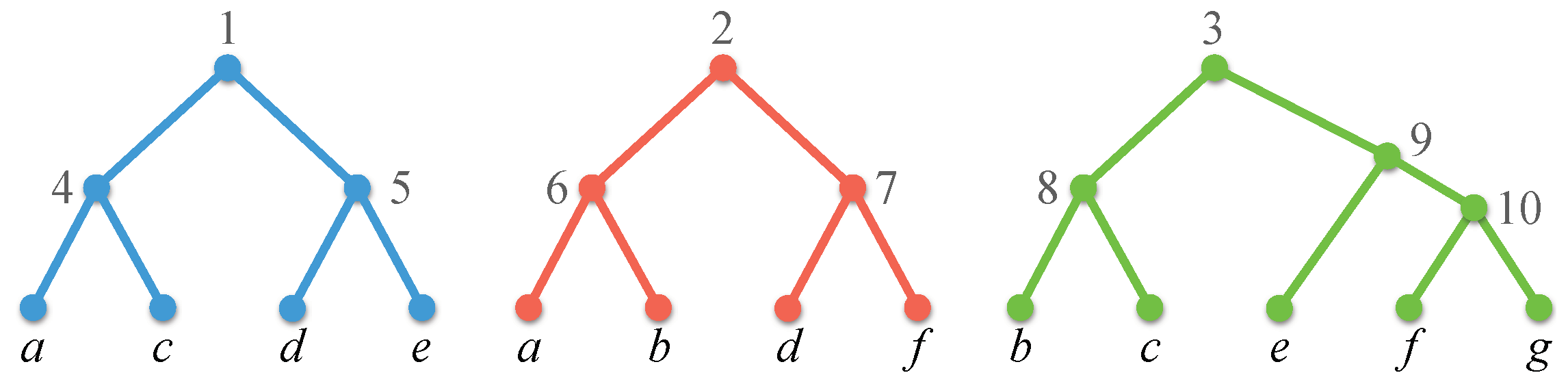
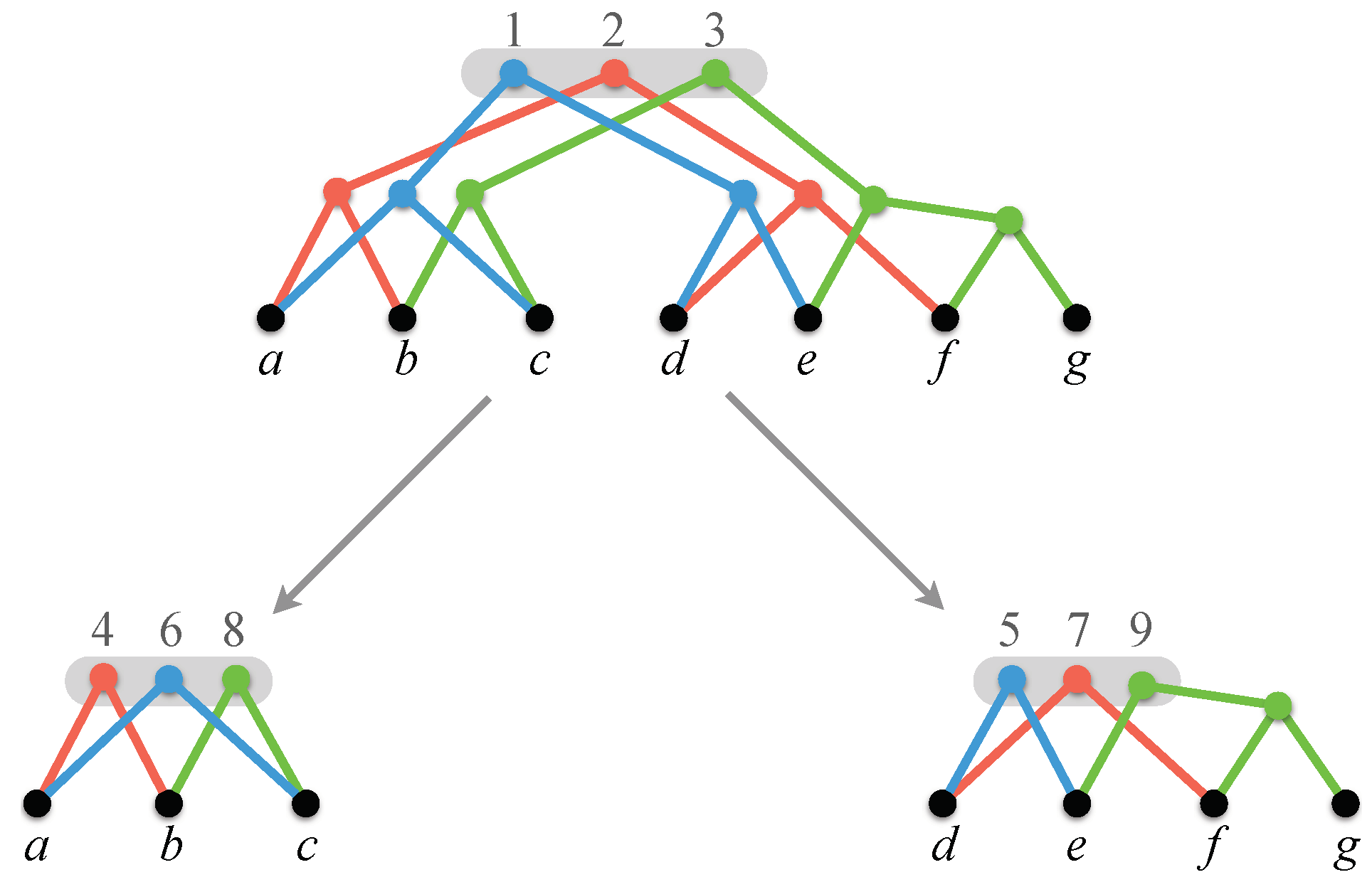
A profile on X is a set $\mathcal{P}=\{{\mathcal{T}}_1,{\mathcal{T}}_2,\cdots ,{\mathcal{T}}_k\}$ where, for each $i\in \left[k\right]$, ${\mathcal{T}}_i=(T_i,{\varphi }_i)$ is a phylogenetic $Y_i$-tree on some set $Y_i\subseteq X$, and ${\bigcup }_{i\in \left[k\right]}{Y}_i=X$ (Figure 1). $V\left(\mathcal{P}\right)$ denotes ${\bigcup }_{i\in \left[k\right]}V\left(T_i\right)$, and $E\left(\mathcal{P}\right)$ denotes ${\bigcup }_{i\in \left[k\right]}E\left(T_i\right)$. The size of $\mathcal{P}$ is $M_{\mathcal{P}}=|V\left(\mathcal{P}\right)|+|E\left(\mathcal{P}\right)|$.

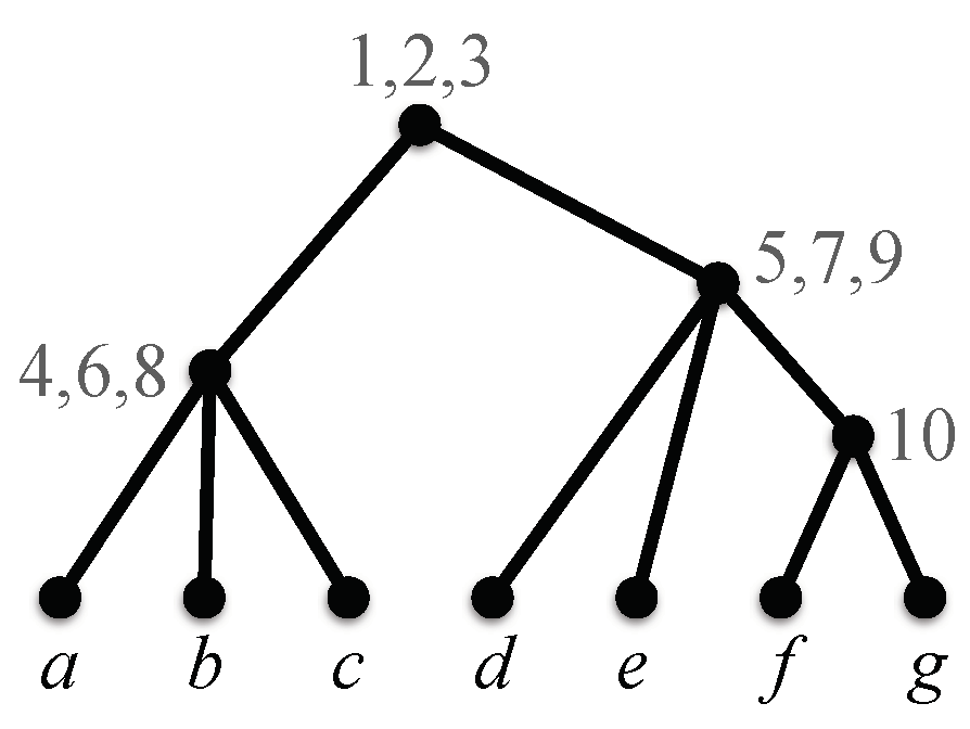
$\mathcal{P}$ is compatible if there exists a phylogenetic X-tree $\mathcal{T}$ such that $\mathcal{T}$ displays ${\mathcal{T}}_i$, for each $i\in \left[k\right]$. Such a tree $\mathcal{T}$, if it exists, is a compatible supertree for $\mathcal{P}$ (Figure 2). The problem of finding a compatible supertree for a profile, or reporting that no such supertree exists, is called the tree compatibility problem.

Profiles consisting of binary trees (and, in particular, rooted triples) are common in practice. As Figure 1 and Figure 2 show, a compatible supertree for a profile of binary trees need not itself be binary.

Suppose $\mathcal{T}$ is a compatible supertree for profile $\mathcal{P}$. It follows from the definition of the notion of “displays” that, for any cluster present in some tree in $\mathcal{P}$, there is a corresponding cluster in $\mathcal{T}$. More formally, for each $i\in \left[k\right]$, there exists a mapping ${\sigma }_i$ from $V\left(T_i\right)$ to $V\left(T\right)$ with the following property. For each $v\in V\left(T_i\right)$, $Y_i\left(v\right)=X\left({\sigma }_i\left(v\right)\right)\cap Y_i$ (here, we use the cluster notation of Section 2.1). We say that v maps to ${\sigma }_i\left(v\right)$; see Figure 2. Note that the mapping ${\sigma }_i$ need not be unique.

3.2. The Display Graph

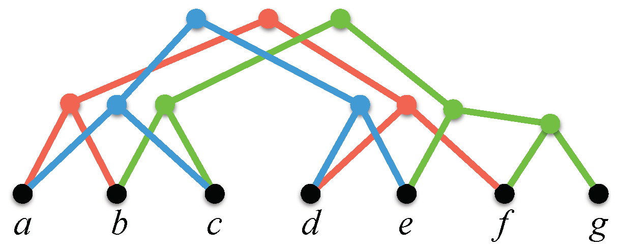
The display graph of a profile $\mathcal{P}$, denoted by $H_{\mathcal{P}}$, is the graph obtained from the disjoint union of the underlying trees $T_1,\cdots ,T_k$ by identifying leaves that have a common label (Figure 3). $H_{\mathcal{P}}$ has $\mathcal{O}\left(M_{\mathcal{P}}\right)$ nodes and edges and can be constructed in $\mathcal{O}\left(M_{\mathcal{P}}\right)$ time.

We refer to a node of $H_{\mathcal{P}}$ that results from identifying multiple leaves as a leaf of $H_{\mathcal{P}}$. Let v be any leaf of $H_{\mathcal{P}}$. The label of v is the common label of the leaves of $\mathcal{P}$ that were identified to create v. We refer to a node v of $H_{\mathcal{P}}$ that is not a leaf as an internal node. A node u in $H_{\mathcal{P}}$ is a child of an internal node v if u is the child of v in some tree in $\mathcal{P}$.

3.3. Incomplete Directed Perfect Phylogeny

Assume $X=\{x_1,\cdots ,x_n\}$, and let $C=\{c_1,\cdots ,c_k\}$ be a set of characters. A character matrix is an $n\times k$ matrix $A=\left[a_{ij}\right]$, where $a_{i,j}\in \{0,1,?\}$. Entry $a_{ij}$ is called the state of taxon $x_i$ on character $c_j$. For each $j\in \left[k\right]$ and each $s\in \{0,1,?\}$, the s-set of character $c_j$ is the set of taxa ${\sigma }_j(A,s)=\{x_i\in X:a_{ij}=s\}$.

A completion of a $\{0,1,?\}$-matrix A is a $\{0,1\}$-matrix B obtained by replacing all the ?s in A by zeroes and ones (thus, ${\sigma }_j(B,?)=\varnothing$ for all $j\in \left[k\right]$). A perfect phylogeny for a completion B of A is a phylogenetic X-tree $\mathcal{T}$ such that ${\sigma }_j(B,1)\in \mathrm{Cl}\left(\mathcal{T}\right)$ for every $j\in \left[k\right]$. If such a tree $\mathcal{T}$ exists, we call it a perfect phylogeny for A as well.

The input to the incomplete directed perfect phylogeny problem (IDPP) is an $n\times k$$\{0,1,?\}$-matrix A. The problem is to find a perfect phylogeny for A or report that no perfect phylogeny exists.

For each $j\in \left[k\right]$, we say that column j of A is trivial if $|{\sigma }_j(A,1)|<2$ or $|{\sigma }_j(A,0)|<1$. Let $A^{\prime }$ be the matrix obtained from A by striking out all trivial columns. It is straightforward to show that A has a perfect phylogeny if and only if A does. Thus, in the the rest of the paper, we assume that A contains no trivial columns.

3.4. The Relationship between Tree Compatibility and IDPP

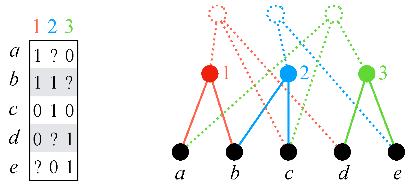
Given an instance A of IDPP, let us define a profile ${\mathcal{P}}_A=\{{\mathcal{T}}_1,\cdots ,{\mathcal{T}}_k\}$ as follows. For each $j\in \left[k\right]$, ${\mathcal{T}}_j$ is the phylogenetic $Y_j$-tree where $Y_j={\sigma }_j(A,0)\cup {\sigma }_j(A,1)$ and where $\mathrm{Cl}\left({\mathcal{T}}_j\right)$ contains only one non-trivial cluster: ${\sigma }_j(A,1)$ (Figure 4).

Lemma 1.

An instance A of IDPP has a perfect phylogeny if and only if ${\mathcal{P}}_A$ is a compatible profile.

Proof. 

We claim that a phylogenetic X-tree $\mathcal{T}$ is a perfect phylogeny for A if and only if $\mathcal{T}$ displays ${\mathcal{T}}_j$ for each $j\in \left[k\right]$; that is, if and only if $\mathcal{T}$ is a compatible supertree of ${\mathcal{P}}_A$.

Indeed, $\mathcal{T}$ is a perfect phylogeny for A if and only if there is a completion B of A such that ${\sigma }_j(B,1)\in \mathrm{Cl}\left(\mathcal{T}\right)$ for every $j\in \left[k\right]$. This holds if and only if, for each $j\in \left[k\right]$, ${\sigma }_j(A,1)={\sigma }_j(B,1)\cap Y_j\in \mathcal{T}|Y_j$, where $Y_j={\sigma }_j(A,0)\cup {\sigma }_j(A,1)$. Since ${\sigma }_j(A,1)$ is the only non-trivial cluster in ${\mathcal{T}}_j$, this is equivalent to saying that $\mathcal{T}$ displays ${\mathcal{T}}_j$. □

4. Algorithms for Tree Compatibility and Incomplete Directed Perfect Phylogeny

4.1. Tree Compatibility

$\mathtt{BuildNT}$ (Algorithm 1) builds a compatible supertree for a profile $\mathcal{P}$ by traversing the display graph $H_{\mathcal{P}}$ top-down, starting from the roots of the input trees, successively decomposing $H_{\mathcal{P}}$ into subgraphs that correspond to subtrees of the compatible supertree [10]. If it is impossible to decompose $H_{\mathcal{P}}$, the algorithm reports that $\mathcal{P}$ is incompatible. To explain $\mathtt{BuildNT}$ in more detail, we need some definitions and notation. Figure 5 illustrates several of these notions.

A position in $H_{\mathcal{P}}$ is a vector $U=\left(U\right(1),\cdots ,U(k\left)\right)$, where $U\left(i\right)\subseteq V\left({\mathcal{T}}_i\right)$, for each $i\in \left[k\right]$. For each $i\in \left[k\right]$, let ${\mathrm{Desc}}_i\left(U\right)=\{v\in V\left(H_{\mathcal{P}}\right):v\mathrm{is}\mathrm{a}\mathrm{descendant}\mathrm{of}{v}^{\prime }\mathrm{in}{\mathcal{T}}_i\mathrm{for}\mathrm{some}{v}^{\prime }\in U\left(i\right)\}$, and let ${\mathrm{Desc}}_{\mathcal{P}}\left(U\right)={\bigcup }_{i\in \left[k\right]}{\mathrm{Desc}}_i\left(U\right)$. Note that, since labels may be shared among trees and $H_{\mathcal{P}}$ is obtained by identifying leaves with the same label, we may have $\mathrm{Desc}\left(U\right(i\left)\right)\cap \mathrm{Desc}\left(U\right(j\left)\right)\ne \varnothing$, for $i,j\in \left[k\right]$ with $i\ne j$.

A position U is valid if the following holds for each $i\in \left[k\right]$.

• If $|U(i)|\ge 2$, then the elements of $U\left(i\right)$ are siblings in ${\mathcal{T}}_i$ and
• ${\mathrm{Desc}}_i\left(U\right)={\mathrm{Desc}}_{\mathcal{P}}\left(U\right)\cap V\left({\mathcal{T}}_i\right)$.

For any valid position U, let $H_{\mathcal{P}}\left(U\right)$ denote the subgraph of $H_{\mathcal{P}}$ induced by ${\mathrm{Desc}}_{\mathcal{P}}\left(U\right)$. Then, $H_{\mathcal{P}}\left(U\right)$ is the subgraph of $H_{\mathcal{P}}$ obtained by deleting all nodes in $V\left(H_{\mathcal{P}}\right)\setminus {\mathrm{Desc}}_{\mathcal{P}}\left(U\right)$, along with all incident edges [10].

Let U be a valid position, and let v be a vertex in U. Then, v is semi-universal in U if $U\left(i\right)=\left\{v\right\}$, for every $i\in \left[k\right]$ such that $v\in V\left({\mathcal{T}}_i\right)$. Let $S\left(U\right)$ denote the set of semi-universal labels in U. The successor of U is the position $U^{\prime }$ such that, for each $i\in \left[k\right]$, if $U\left(i\right)=\left\{v\right\}$, for some $v\in S\left(U\right)$, then $U^{\prime }\left(i\right)={\mathrm{Ch}}_i\left(v\right)$, where ${\mathrm{Ch}}_i\left(v\right)$ denotes the set of children of v in $V\left({\mathcal{T}}_i\right)$; otherwise, $U^{\prime }\left(i\right)=U\left(i\right)$.

The root position is the position $U_{\mathrm{root}}$ where, for each $i\in \left[k\right]$, $U_{\mathrm{root}}\left(i\right)$ is a singleton containing $r\left(T_i\right)$. It is obvious that $U_{\mathrm{root}}$ is valid, that ${\mathrm{Desc}}_{\mathcal{P}}\left(U_{\mathrm{root}}\right)=V\left(H_{\mathcal{P}}\right)$, that $H_{\mathcal{P}}\left(U_{\mathrm{root}}\right)=H_{\mathcal{P}}$, and that every vertex in $U_{\mathrm{root}}$ is semi-universal.

The key idea behind $\mathtt{BuildNT}$ is that if $H_{\mathcal{P}}\left(U\right)$ is connected, then all semi-universal nodes in U can map to the same node $r_U$ in a compatible supertree $\mathcal{T}$ for $\mathcal{P}$. The set of labels in the cluster at $r_U$ is precisely the set of labels that appear in $H_{\mathcal{P}}\left(U\right)$. Further, each connected component of $H_{\mathcal{P}}\left(U^{\prime }\right)$ corresponds to a distinct subtree of $r_U$ in $\mathcal{T}$.

$\mathtt{BuildNT}$ uses a first-in first-out queue Q to store pairs $\langle U,\mathrm{pred}\rangle$, where U is a valid position in $\mathcal{P}$ and $\mathrm{pred}$ is a reference to the parent of the node corresponding to U in the supertree built so far. $\mathtt{BuildNT}$ initializes Q to contain the starting position, $U_{\mathrm{root}}$, with a null parent. Each iteration of the while loop of Lines 3–15 starts by de-queuing a pair $\langle U,\mathrm{pred}\rangle$. Line 5 computes the set S of semi-universal labels in U. It can be shown that if S is empty, then $\mathcal{P}$ is incompatible [10]. This case is handled in Lines 6–7. If S is not empty, the algorithm creates a tentative root $r_U$ labeled by S for the tree ${\mathcal{T}}_U$ for ${\mathrm{Desc}}_{\mathcal{P}}\left(U\right)$ and links $r_U$ to its parent (Line 8). If S consists of exactly one element that is a leaf in $H_{\mathcal{P}}$, then $r_U$ is a potential leaf in the output tree $\mathcal{T}$. We set the label of $r_U$ appropriately, skip the rest of the current iteration of the while loop, and continue to the next iteration (Lines 9–11). Line 12 replaces U by its successor with respect to S. Lines 14–15 enqueue each of $U|W_1,U|W_2,\cdots ,U|W_p$—where $U|W_j$ denotes the position $(U\left(1\right)\cap W_j,\cdots ,U\left(k\right)\cap W_j)$—along with $r_U$, for processing in subsequent iterations. If the while loop terminates without detecting incompatibility, $\mathtt{BuildNT}$ returns the phylogenetic X-tree $\mathcal{T}=(T,\varphi )$, where T is the tree with root $r_{U_{\mathrm{root}}}$ and $\varphi$ is the labeling function constructed in Line 10.

Algorithm 1:$\mathtt{BuildNT}\left(\mathcal{P}\right)$

There are two main contributors to the running time of $\mathtt{BuildNT}$. The first is the time to compute the successor of U along with the connected components of $H_{\mathcal{P}}\left(U\right)$ in Lines 12–13. Let $U^{\prime }$ be the successor of U with respect to $S\left(U\right)$. Then, $H_{\mathcal{P}}\left(U^{\prime }\right)$ can be obtained from $H_{\mathcal{P}}\left(U\right)$ by doing the following for each $v\in S\left(U\right)$: (1) for each $i\in \left[k\right]$ such that $U\left(i\right)=\left\{v\right\}$, delete all edges between v and ${\mathrm{Ch}}_i\left(v\right)$; (2) delete v. Using HDT (Section 2.2.2), each deletion takes $O\left({log}^2{M}_{\mathcal{P}}\right)$ amortized time. Since the total number of edge and node deletions is $\mathcal{O}\left(M_{\mathcal{P}}\right)$, the total work done in these lines is $\mathcal{O}\left(M_{\mathcal{P}}{log}^2{M}_{\mathcal{P}}\right)$. If instead of HDT, we use its single-level version, HDT(0) (Section 2.2.3), then, by Proposition 1, the running time is $\mathcal{O}(M_{\mathcal{P}}+slog{M}_{\mathcal{P}})$, where s is the number of edge scans performed by $\mathtt{BuildNT}$ over its entire execution.

The other main contributor to the running time of $\mathtt{BuildNT}$ is maintaining the semi-universal nodes of the various components that result from edge deletions, so that the labels can be quickly retrieved in Line 5. Suppose this information is known for the connected component being processed in the current iteration of $\mathtt{BuildNT}$’s while loop. When an edge deletion splits a connected component of $H_{\mathcal{P}}$ in two, the algorithm traverses the smaller component to update the set of semi-universal vertices in that component. It can be shown that, over the entire execution of $\mathtt{BuildNT}$, any given vertex is visited $\mathcal{O}(log{M}_{\mathcal{P}})$ times, spending $O\left(1\right)$ time per visit. Thus, the total time spent to update semi-universal vertex information throughout the entire execution of the algorithm is $\mathcal{O}(M_{\mathcal{P}}log{M}_{\mathcal{P}})$.

The following result is adapted from [10].

Theorem 1.

Let $\mathcal{P}$ be a profile. If $\mathcal{P}$ is compatible, then $\mathtt{BuildNT}\left(\mathcal{P}\right)$ returns a tree T that displays $\mathcal{P}$; otherwise, $\mathtt{BuildNT}\left(\mathcal{P}\right)$ returns $\mathtt{incompatible}$. When implemented using HDT, the running time of $\mathtt{BuildNT}\left(\mathcal{P}\right)$ is $\mathcal{O}\left(M_{\mathcal{P}}{log}^2{M}_{\mathcal{P}}\right)$. When implemented using HDT$\left(0\right)$, the running time is $\mathcal{O}((M_{\mathcal{P}}+s)·log{M}_{\mathcal{P}})$, where s is the total number of edge scans performed over the entire execution of $\mathtt{BuildNT}\left(\mathcal{P}\right)$.

4.2. IDPP

By Lemma 1 (Section 3.4), we can solve any instance A of IDPP by converting it to a profile ${\mathcal{P}}_A$ and then using $\mathtt{BuildNT}$ to determine if there exists a tree $\mathcal{T}$ that displays ${\mathcal{P}}_A$. If $\mathcal{T}$ exists, then it must be a perfect phylogeny for A. Otherwise, no perfect phylogeny for A exists.

In [13], Pe’er et al. gave a specialized algorithm for IDPP; we refer to their algorithm as $\mathtt{PPSS}$. $\mathtt{PPSS}$ can be viewed as a variation of $\mathtt{BuildNT}$, with two key differences, which we explain next. Let A be an instance of IDPP, and let $\mathcal{P}={\mathcal{P}}_A$.

• $\mathtt{PPSS}$ works with $H_{\mathcal{P}}\setminus U_{\mathrm{root}}$ instead of $H_{\mathcal{P}}$. This is correct, since every vertex in $U_{\mathrm{root}}$ is semi-universal. Let m denote the number of ones in A. Then, $H_{\mathcal{P}}\setminus U_{\mathrm{root}}$ has $n+k$ nodes and m edges (see Figure 4). Note that m can be considerably smaller than $M_{\mathcal{P}}$, since $H_{\mathcal{P}}$ contains edges for both the zeroes and the ones of A. Since the number of edge deletions is $\mathcal{O}\left(m\right)$, the total work to maintain the connected components throughout the entire execution of $\mathtt{PPSS}$ is $\mathcal{O}\left(m{log}^2(n+k)\right)$, if we use HDT, and $\mathcal{O}\left(\right(m+s)·log(n+k\left)\right)$, if we use HDT(0).
• $\mathtt{PPSS}$ updates the set of semi-universal nodes after it computes a successor position. It does so by traversing each of the resulting connected components. Each such traversal takes $O(n+k)$ time, assuming the connected components are represented by a spanning forest. The number of times a successor position is computed is bounded by the number of edges in the final phylogeny, which is $\mathcal{O}(min\{n,k\left\}\right)$. Thus, the total work performed by $\mathtt{PPSS}$ in updating semi-universal nodes is $\mathcal{O}\left(nk\right)$. In contrast, $\mathtt{BuildNT}$ updates the set of semi-universal nodes while computing a successor position; i.e., after each tree edge deletion.

The running time of $\mathtt{PPSS}$ is therefore $\mathcal{O}(nk+m{log}^2(n+k))$, if $\mathtt{PPSS}$ is implemented using HDT, and $\mathcal{O}(nk+(m+s)·log(n+k\left)\right)$, if we use HDT(0) (we note that a somewhat better running time can be achieved if $H_{\mathcal{P}}$ is extremely dense [13]).

5. Experiments with Tree Compatibility

We implemented $\mathtt{BuildNT}$ using treaps [23] to represent ET trees, as done by Iyer et al. [22]. We refer to our program, written in C++, as FCT (https://zenodo.org/record/2114273#.XA7iIy2ZPOQ). FCT implements level truncation (Section 2.2.3), allowing us to specify the maximum level to which an edge can be promoted in HDT. Two extreme cases are of special interest. One permits HDT to promote edges up to the maximum allowed level $\lfloor {log}_{2}n\rfloor$. We refer to the version of FCT that implements this strategy as FCT(1). The other extreme is to disallow edge promotions entirely; i.e., we use HDT(0). We refer to this version of FCT as FCT$\left(0\right)$.

We ran all experiments on a device with a 2.7-GHz dual core-Intel Core i5 processor and 8-G 1866-MHz LPDDR3 memory. The times reported here do not account for the initialization of the data structures.

5.1. Real Datasets

Table 1. Runtime on real datasets.

	Legumes	Seabirds	Mammals
FCT(0)	0.0277 s	0.0051 s	0.1327 s
FCT(1)	0.0926 s	0.0192 s	0.3623 s

shows the running times, in seconds, of FCT(0) and FCT(1) on three well-known datasets: Legumes (471 taxa, 22 trees) [24], Seabirds (121 taxa; 7 trees) [25], and Placental Mammals (116 taxa; 726 trees) [26]. In all three cases, FCT(0) and FCT(1) terminated quickly and correctly reported incompatibility, but FCT(0) was always considerably faster.

5.2. Generating Simulated Data

An inherent limitation of testing FCT on real datasets, such as the three considered in the previous section, is that they are often incompatible. Incompatible inputs do not exercise FCT as thoroughly as we would like, since the program is likely to terminate early, leaving large parts of $H_{\mathcal{P}}$ unexamined. In order to conduct more extensive tests, we implemented a generator of compatible input profiles.

Our generator begins by producing a random phylogenetic X-tree $\mathcal{T}$ on n leaves whose internal nodes have a user-specified degree $D\ge 2$, except possibly for the root, which may have degree less than D. The generator produces a compatible profile $\mathcal{P}=\{{\mathcal{T}}_1,\cdots ,{\mathcal{T}}_k\}$, by restricting $\mathcal{T}$ to different subsets of X. We focus on two types of profiles.

• Profiles of rooted triples. We start from a binary phylogenetic X-tree $\mathcal{T}$. For each $i\in \left[k\right]$, we obtain ${\mathcal{T}}_i$ by restricting $\mathcal{T}$ to a distinct three-element subset of X. We have $n-2\le k\le \left(\genfrac{}{}{0pt}{}{n}{3}\right)$. If $k=n-2$, we choose $\mathcal{P}$ to be a set of rooted triples that defines $\mathcal{T}$. That is, $\mathcal{T}$ is the only compatible supertree for $\mathcal{P}$ (the existence of such sets of triples is a folklore theorem in phylogenetics). If $k=\left(\genfrac{}{}{0pt}{}{n}{3}\right)$, $\mathcal{P}$ consists of every rooted triple that can be obtained by restricting $\mathcal{T}$ to a three-element subset of X. In the latter case, we say that $\mathcal{P}$ is a complete set of rooted triples.
• Profiles of phylogenetic trees of specified degree. We start from a phylogenetic X-tree $\mathcal{T}$ whose nodes have degree D. We obtain $\mathcal{P}$ by restricting $\mathcal{T}$ to k randomly-chosen subsets of X; each label is chosen to be in a set with probability ${\displaystyle \frac{1}{2}}$.

We conducted a series of tests on simulated datasets. Each reported data point is the average execution time, in seconds, over 30 trials.

5.3. Impact of Level Truncation

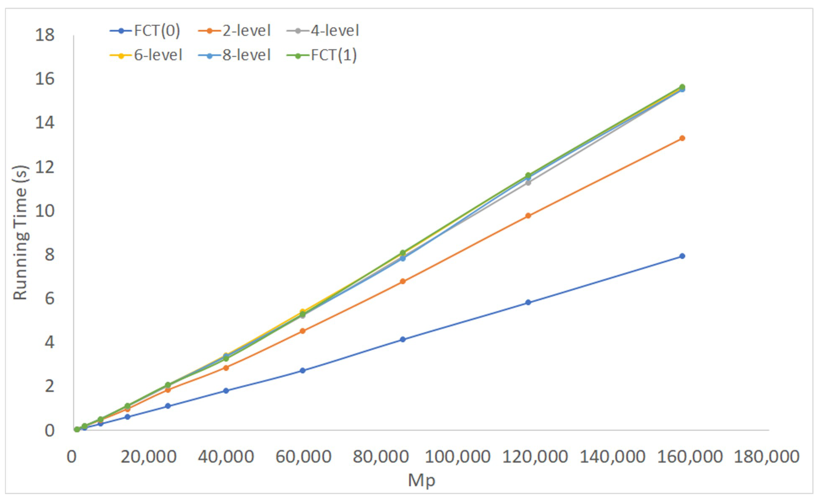
Figure 6 shows the running time of FCT on complete sets of triples, with maximum truncation levels set to 1 (i.e., FCT(0)), 2, 4, 6, 8, and $\lfloor logn\rfloor$ (i.e., FCT(1)). The number of taxa, n, ranged from 10–55 with increments of 5. Thus, $730\le M_{\mathcal{P}}\le 157,465$.

Observe that going beyond 4 levels made little difference. Indeed, beyond Level 1, the difference is small. This observation is consistent with the intuition that the higher levels of HDT tend to be sparsely populated and are rarely used.

FCT(0) is the clear winner in these tests. The same was true for every dataset we considered, whether they were profiles of rooted triples or profiles of more general phylogenetic trees (Figures S1–S7 in the Supplementary Materials). Thus, in the rest of this section, we focus our attention on HDT(0).

5.4. Worst-Case Time versus Empirically-Observed Time

By Theorem 1, the worst-case time of FCT(0) depends on the number of edge scans performed when searching for replacement edges. A naive estimate yields a worst-case bound of $O\left(M_{\mathcal{P}}^2\right)$ for this number: $O\left(M_{\mathcal{P}}\right)$ edge deletions, each requiring $O\left(M_{\mathcal{P}}\right)$ scans. This implies a time bound of $O(M_{\mathcal{P}}^{2}log{M}_{\mathcal{P}})$ for the entire execution of FCT(0). In contrast, we now present evidence that FCT(0)’s performance in practice may be closer to $O(M_{\mathcal{P}}log{M}_{\mathcal{P}})$ than to its worst-case bound.

Performance on Rooted Triples

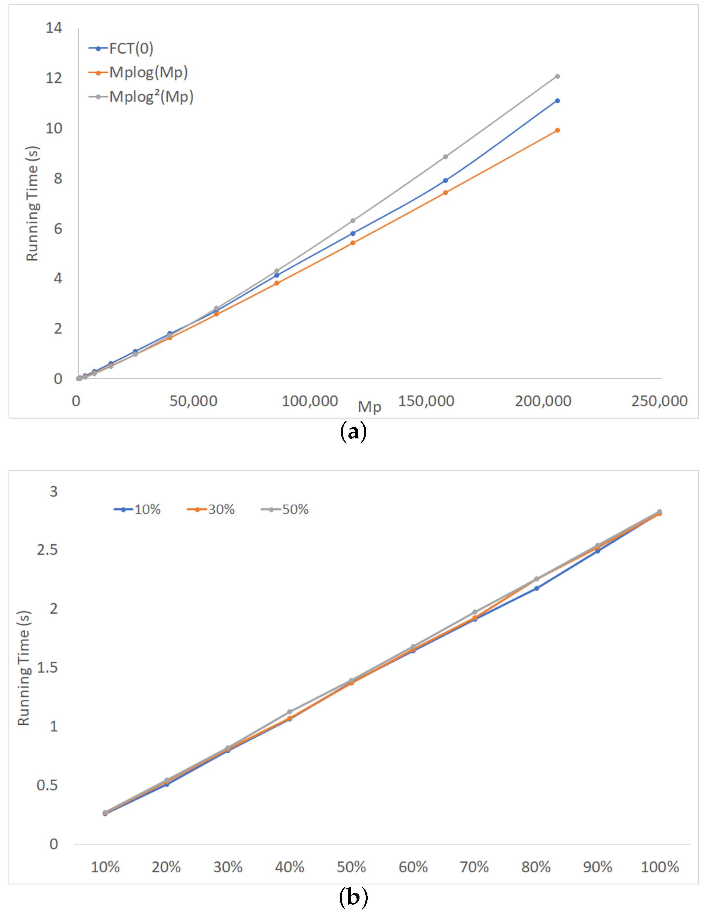
Figure 7a shows the running time of FCT(0) on complete sets of triples. The number of taxa, n, varied from 5–60 with increments of 5, and $M_{\mathcal{P}}$ varied from 65–205,380. Also plotted in that figure are the functions $c_1·M_{\mathcal{P}}log{M}_{\mathcal{P}}+c_2$ and $c_1^{\prime }·M_{\mathcal{P}}{log}^2{M}_{\mathcal{P}}+c_2^{\prime }$, where $c_1$, $c_2$, $c_1^{\prime }$, and $c_2^{\prime }$ are appropriate constants. The plot suggests that, in practice, the running time of FCT(0) was far better than the above-mentioned worst case and may be close to $O\left(M_{\mathcal{P}}{log}^2{M}_{\mathcal{P}}\right)$.

We also explored the effect of altering the balance factor of the binary phylogenetic X-tree $\mathcal{T}$ from which the triples wee derived (the balance factor is the ratio $\alpha$ of the size of the smaller subtree to that of the larger subtree: a binary phylogenetic tree is balanced when $\alpha =0.5$). Figure 7b shows the results of running FCT(0) on the profile of triples on $n=40$ labels for three balance factors: 10%, 30%, and 50%. The x-axis indicates the percentage of the maximum possible number of triples, $\left(\genfrac{}{}{0pt}{}{n}{3}\right)$, included in a profile. The percentage varied from 10%–100%, with increments of 10%. The running time of FCT(0) appeared to be close to linear in the number of triples; the balance factor has a negligible impact. Thus, in the rest of this section, we use starting trees $\mathcal{T}$ that are, on average, balanced.

5.5. Performance on Profiles of More General Phylogenetic Trees

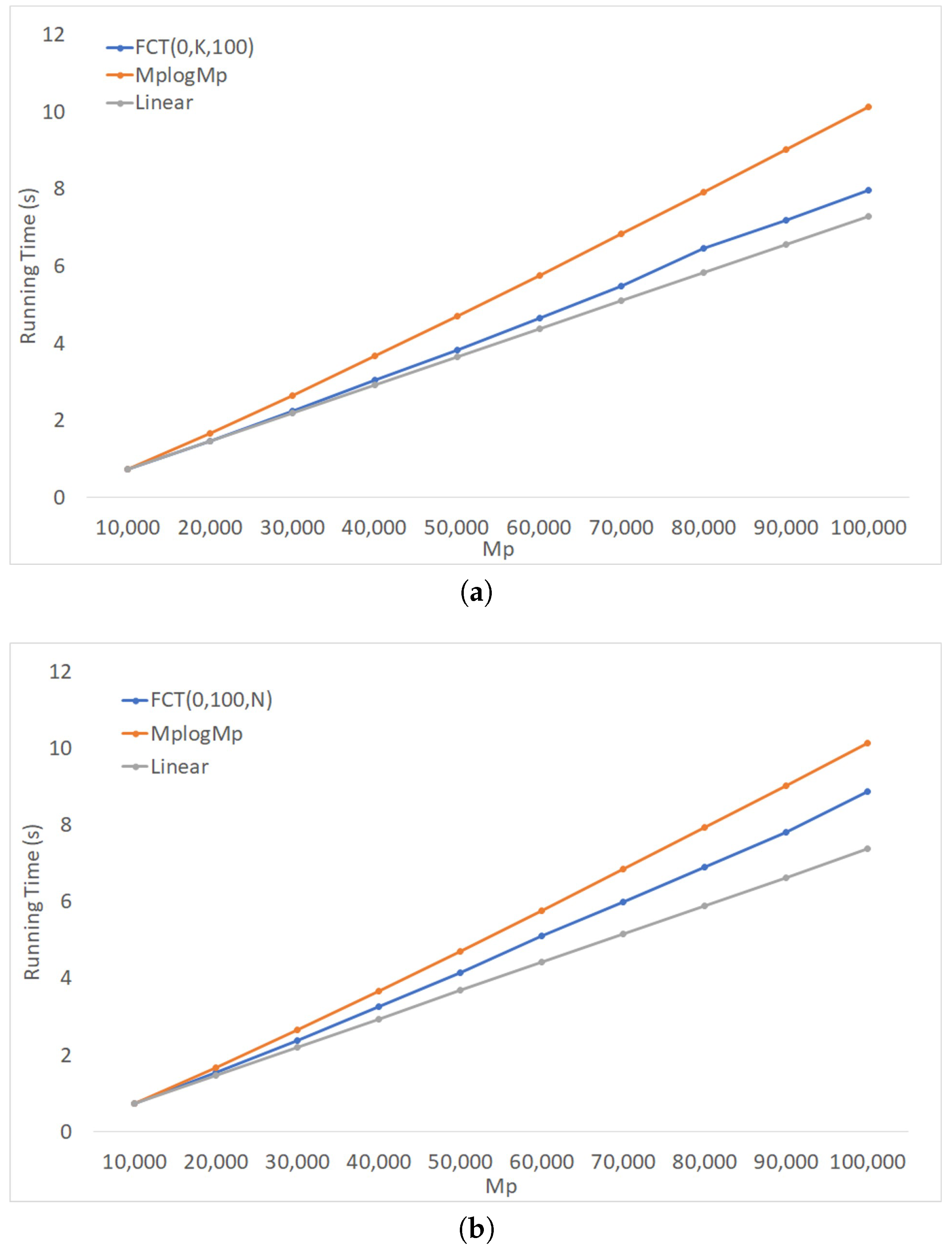
Figure 8a shows the running time of FCT(0) on profiles of binary trees when the number, k, of trees was fixed at 100 and the number, n, of taxa varied from 100–1000, with increments of 100. Figure 8b shows the performance of FCT(0) on profiles of binary trees when the number of taxa was fixed at 100, while k varied from 100–1000 with increments of 100. Both figures compare the empirical performance against $O\left(M_{\mathcal{P}}\right)$ and $O(M_{\mathcal{P}}log{M}_{\mathcal{P}})$ curves, using the product $n\times k$ as a proxy for $M_{\mathcal{P}}$. Although the running time of FCT(0) grew non-linearly, its behavior appeared to be close to $O(M_{\mathcal{P}}log{M}_{\mathcal{P}})$.

We also studied the performance of FCT(0) on profiles of trees of degrees 4 and 7. The results, which appear in Figures S11 and S12 of the Supplementary Materials, were qualitatively similar to those for binary trees. Note that a greater number of higher degree internal nodes can be beneficial for dynamic connectivity data structures based on spanning forests: an abundance of such nodes increased the number of non-tree edges in $H_{\mathcal{P}}$, which were trivial to delete (see Section 2.2). We return to this issue in Section 7.

5.6. Connectivity Testing versus Maintaining Semi-Universal Labels

Throughout all of our experiments, connectivity testing took on average slightly more than 50% of FCT(0)’s running time. FCT(0) spent most of its rest time maintaining semi-universal nodes. As noted in Section 4, the time to do the latter was asymptotically $\mathcal{O}(M_{\mathcal{P}}log{M}_{\mathcal{P}})$. As one might expect, there was less variability in this aspect than in dynamic connectivity testing.

6. Experiments with IDPP

We implemented $\mathtt{PPSS}$, the IDPP algorithm of Pe’er et al. described in Section 4.2; we refer to our implementation as FPP (https://zenodo.org/record/2115972#.XA7mey2ZPOQ). Like FCT, FPP was implemented in C++ and used treaps to represent ET trees. There were two versions of FPP: FPP(1) used the full implementation of HDT, which allowed promotion of edges up to level $\lfloor {log}_{2}n\rfloor$; FPP(0) used HDT(0). We ran our tests on the same machine used to obtain the results reported in Section 5.

6.1. Simulated Datasets

To generate a random instance of IDPP, our generator proceeded as follows. We started from a Prüfer code of length of $2n-2$, which defines a unique tree $\mathcal{T}$ with n leaves (taxa) and n internal nodes (characters) [27,28]. We rooted $\mathcal{T}$ at a randomly-chosen node and then translated the tree into an $n\times n$ zero-one matrix C that encoded the clusters in $\mathcal{T}$ (each column of C corresponds to a cluster; a one indicates that a taxon is present in the cluster, a zero that it is absent). We obtained a seed matrix B by duplicating columns in C. We built different instances of IDPP from a seed matrix by converting a randomly-chosen set of zero- and/or one-entries to question marks.

The generator can build seed matrices of different densities, where the density of a matrix is the ratio of its number of ones to its total number of entries. Let us call a column of C trivial if all its entries are one. We built a seed matrix B by duplicating non-trivial columns where the percentage of ones was above a specified threshold. If the threshold is 25%, we say that the matrix has medium density; if the threshold is 50%, we say that the matrix has high density. We also consider matrices generated without a mandatory threshold, allowing any columns to be duplicated; we refer to such instances as low-density matrices. There is a caveat: The process that we use to generate the starting tree $\mathcal{T}$ may lead to a matrix C where no non-trivial column has the mandatory threshold. If this was the case, we reduced the threshold and tried again. For medium-density matrices, if 25% failed, we successively tried 20% and 10%. For high-density matrices, if 50% failed, we tried 40%, 30%, 20%, and 10%.

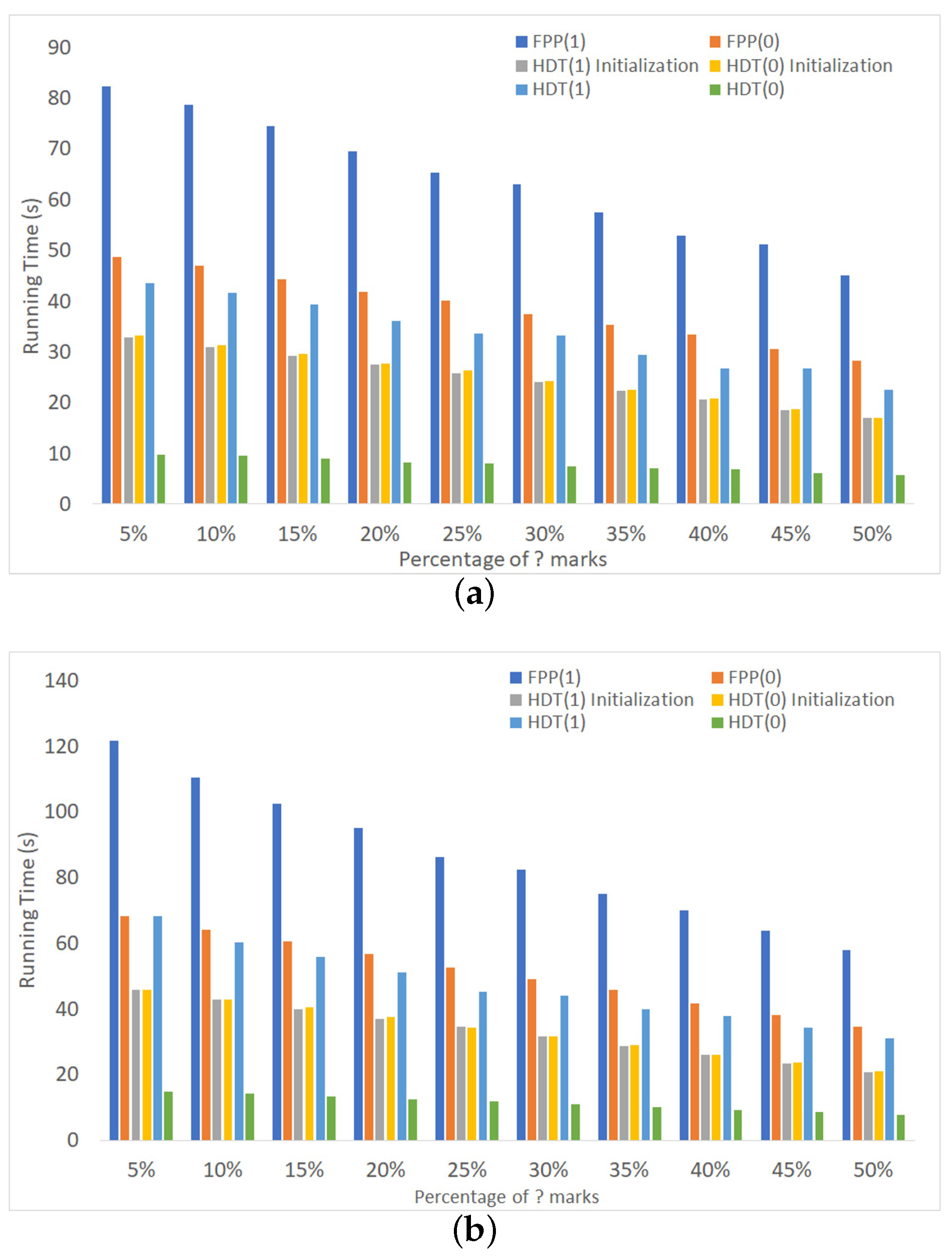
Figure 9 shows the execution time of FPP(1) and FPP(0) on medium- and high-density matrices. In both cases, n and k are fixed. For each data point reported, we started with a particular (random) seed matrix and then generated multiple IDPP instances by replacing a certain percentage of ones in the seed matrix by question marks. To be consistent, we also converted the same percentage of zeroes to question marks. The percentage ranged from 5%–50% with increments of 5%. The figures also show the time needed to initialize the connectivity data structures and the total time spent on manipulating these structures.

Without exception, the experiments showed that there was no benefit to enabling edge promotion in HDT; a single level suffices. A more extensive set of results, leading to the same conclusion, is reported in the Supplementary Materials (Figure S13).

6.2. Solving IDPP via Tree Compatibility

As explained in Section 3.4 and Section 4.2, any instance A of IDPP can be solved by transforming it into a profile ${\mathcal{P}}_A$ and then checking if ${\mathcal{P}}_A$ is compatible.

Table 2. Comparison between execution time (in seconds) of the tree compatibility algorithm on transformed IDPP and original IDPP on high-density matrices of order $100\times 2000$.

	5%	10%	15%	20%	25%	30%	35%	40%	45%	50%
FCT(0)	10.07	10.00	9.87	9.61	9.52	9.41	9.36	9.07	9.05	8.80
FPP(0)	6.43	6.48	6.38	6.32	6.43	5.68	6.30	6.55	6.44	6.12
Connectivity (FCT)	3.37	3.37	3.32	3.24	3.28	3.22	3.30	3.16	3.15	3.07
Connectivity (FPP)	1.38	1.36	1.33	1.28	1.36	1.26	1.35	1.42	1.38	1.30

compares the running time of FPP(0) against that of FCT(0) applied to the corresponding instance of tree compatibility, on high-density input matrices of order $100\times 2000$. As in Figure 9, we varied the percentage of zeroes and ones converted to question marks from 5%–50% with increments of 5%. The table also shows the time the programs spent on maintaining connectivity information. FPP(0) was uniformly faster than FCT(0). Much of this speedup can be attributed to the smaller amount of time FPP(0) spent in connectivity-related work compared to FCT(0). This reflects the fact that the former operates on a graph that contains edges only for the one-entries of A, whereas the latter works with the entire display graph of ${\mathcal{P}}_A$, which contains edges for every one and zero-entry of A. We found similar results for low-density matrices (Supplementary Materials, Table S2).

7. Analysis

In our experiments, the most striking and consistent observation was the effectiveness of HDT(0) for both compatibility testing and IDPP, across the entire range of inputs considered. A partial explanation is that HDT(0) incurs far less overhead than HDT. This, however, does not fully explain why the running time of FCT(0) was close to $O(M_{\mathcal{P}}log{M}_{\mathcal{P}})$ in practice. Theorem 1 indicates that this performance may be tied to the small number of edge scans performed throughout the execution of the algorithms. Here, we explore this issue in more detail. First, we break down in more detail the factors that affect the performance of HDT(0) in $\mathtt{BuildNT}$ and $\mathtt{PPSS}$.

For each vertex $v\in V\left(H_{\mathcal{P}}\right)$, let $d_v$ denote the number of children of v. At any stage of its execution, $\mathtt{BuildNT}$ maintains a graph H obtained from $H_{\mathcal{P}}$ through edge and node deletions. Because these deletions are performed top-down, the number of edges incident on any node v in H is at most $d_v$.

Lemma 2.

Let $e=(u,v)$ be a tree edge in the current spanning forest F maintained by HDT(0) during the execution of $\mathtt{BuildNT}$ (or $\mathtt{PPSS}$), and let $T_u$ and $T_v$ be the two trees that result from deleting e from the tree in F that contains e. Assume, without loss of generality, that $|V\left(T_u\right)|\le |V\left(T_v\right)|$. Then, searching for a replacement edge for e requires scanning at most $2+{\sum }_{w\in V\left(T_u\right)}(d_w-1)$ non-tree edges.

Proof. 

We claim that the number of non-tree edges scanned is at most one more than the number of edges with both endpoints in $T_u$. To see why, note that the scan for a replacement edge stops as soon as either (i) we encounter an edge that has one endpoint, x, in $T_u$ and the other, y, outside $T_u$ (and, thus, $(x,y)$ is a replacement edge) or (ii) we find that all non-tree edges incident on $T_u$ have both of their endpoints in $T_u$ (and, thus, no replacement edge exists). To complete the proof, we argue that the number of non-tree edges with both endpoints in $T_u$ is at most $1+{\sum }_{w\in V\left(T_u\right)}{d}_w$.

Let $m_u$ be the total number of tree and non-tree edges incident on $V\left(T_u\right)$. Then, $m_u\le {\sum }_{w\in V\left(T_u\right)}{d}_w$. The number of tree edges with both endpoints in $V\left(T_u\right)$ is $m_u^{\prime }=|V\left(T_u\right)|-1$. The number of non-tree edges is thus $m_u-m_u^{\prime }\le {\sum }_{w\in V\left(T_u\right)}{d}_w-(|V\left(T_u\right)|-1)\le 1+{\sum }_{w\in V\left(T_u\right)}(d_w-1)$, as claimed. □

Proposition 2.

Let F be the current spanning forest maintained by HDT(0) during the execution of $\mathtt{BuildNT}$ (or $\mathtt{PPSS}$); let v be the semi-universal node being processed during the computation of the next successor position; and let e be the next edge incident on v to be deleted. Then, the following hold.

1. 

Deleting e takes:

(a) 

$\mathcal{O}\left(1\right)$ time if e is a non-tree edge,

(b) 

$\mathcal{O}(log{M}_{\mathcal{P}})$ time if e is the only tree edge incident on v, and

(c) 

$\mathcal{O}(min\{{\sum }_{w\in V\left(T\right)}{d}_w{,|V\left(T\right)|}^2\}·log{M}_{\mathcal{P}})$ time otherwise, where T is the smaller of the two trees created by deleting e from F. In particular, if the input profile consists of binary trees, the time is $\mathcal{O}(|V\left(T\right)|·log{M}_{\mathcal{P}})$.

2. 

Suppose $d_v=2$ and that e is the first edge incident on v that is deleted. Let $e^{\prime }$ be the other edge incident on v. Then, at the time of deletion, $e^{\prime }$ is a tree edge, and deleting it takes $\mathcal{O}(log{M}_{\mathcal{P}})$ time.

Proof. 

(1) Part (a) was noted in Section 2.2.2. For Part (b) observe that if e is the only tree edge incident on v, then deleting e leaves v as an isolated node in the spanning forest; i.e, as a component of size one, and, hence, as the smaller component. Any non-tree edge incident on v must be a replacement edge, and, if such an edge is found, it takes $O(log{M}_{\mathcal{P}})$ time to re-link v to the rest of the forest. Part (c) follows from Lemma 2 and the fact that there are at most $\left(\genfrac{}{}{0pt}{}{|V(T)|}{2}\right)-(|V\left(T\right)|-1)$ edges with both endpoints incident in T. The claim for profiles of binary trees follows by noting that $d_w\le 2$ for every node w.

(2) There are two cases. If $e^{\prime }$ was a tree edge before deleting e, then $e^{\prime }$ remains a tree edge after the deletion of e. If $e^{\prime }$ is a non-tree edge before deleting e, then $e^{\prime }$ must be used as a replacement edge during the deletion of e, so $e^{\prime }$ becomes a tree edge.

HDT(0) deletes $e^{\prime }$ by first splitting, in $\mathcal{O}(log{M}_{\mathcal{P}})$ time, the ET-tree that contains both endpoints of $e^{\prime }$. This leaves vertex v as the sole element in the smaller component, after which the vertex v is simply discarded. □

Proposition 2 points to three key issues that affect the performance of HDT(0) when used in either $\mathtt{BuildNT}$ or $\mathtt{PPSS}$: the number of non-tree edge deletions, the number of tree edge deletions, and the size of the smaller components resulting from tree edge deletions.

For profiles consisting of binary phylogenetic trees (including profiles of triples), Proposition 2(2) implies that at least half of HDT(0)’s tree-edge deletions take $\mathcal{O}(log{M}_{\mathcal{P}})$ time in the worst case. This is faster than the amortized time they take when performed by HDT. Proposition 2(1) notes the downside: the other half of the deletions could be expensive. These observations hold to some extent for profiles consisting of trees of small degree, although the ratio of inexpensive to expensive tree-edge deletions goes down. On the other hand, for larger degree trees, and in particular for the denser inputs generated by IDPP, non-tree edges are relatively abundant. As indicated in Proposition 2(1a), such edges are trivial to delete.

Proposition 2(1c) implies that if the majority of the smaller components resulting from tree edge deletions are very small, then the time that HDT(0) spends on maintaining connectivity information throughout the execution of $\mathtt{BuildNT}$ (or $\mathtt{PPSS}$) will also be small. More precisely, let $e_1,\cdots ,e_{\ell }$ be the successive tree edges deleted by $\mathtt{BuildNT}$ (or $\mathtt{PPSS}$), and let $N_i=min\{|V\left(t_i\right){|}^2,{\sum }_{w\in V\left(t_i\right)}{d}_w\}$, where $t_i$ is the smaller of the two trees of HDT(0)’s spanning forest created by deleting $e_i$. Then, the total time spent in all tree edge deletions is $\mathcal{O}({\sum }_{i=1}^{\ell }{N}_i·log{M}_{\mathcal{P}})$. If, for instance, ${\sum }_{i=1}^{\ell }{N}_i=O(M_{\mathcal{P}}log{M}_{\mathcal{P}})$, then the total time to maintain connectivity information (including the total time for non-tree edge deletions, which take $\mathcal{O}\left(1\right)$ time each) would be $O\left(M_{\mathcal{P}}{log}^2{M}_{\mathcal{P}}\right)$, matching the behavior we observed in Section 5.

In the next sections, we examine separately the three key factors affecting the performance of HDT(0) on $\mathtt{BuildNT}$ and $\mathtt{PPSS}$. Section 7.1 studies the impact of deletion of non-tree edges on overall performance. As one would expect, the number of such deletions increases with the degree of the input trees. Section 7.2 examines the impact of tree-edge deletion. Here, the focus is on the number of edges scanned in searching for a replacement edge. As we shall see, the total number of such edges grows at a rate that seems only slightly super-linear in $M_{\mathcal{P}}$. Section 7.3 studies the size of the smaller components encountered during tree edge deletions. Surprisingly, we find that components of size at most two constitute the overwhelming majority across a wide range of profiles.

7.1. The Impact of Deleting Non-Tree Edges

We first examine the prevalence of non-tree edge deletions and their total contribution to the execution time. Recall that each such deletion takes $\mathcal{O}\left(1\right)$ time (Proposition 2(1a)).

Table 3. FCT(0) on complete sets of triples: Ratio of number of deleted non-tree edges to total number of edges and ratio of time spent on deleting non-tree edges to total HDT execution time.

${\mathit{M}}_{\mathcal{P}}$	65	730	2745	6860	13,825	24,390	39,305	59,320	85,185	117,650
${\displaystyle \frac{\mathit{Num}\left(\mathit{NTE}\right)}{\mathit{Num}\left(E\right)}}$	9.25%	19.51%	21.88%	21.08%	22.49%	23.00%	23.20%	22.49%	23.05%	23.13%
${\displaystyle \frac{\mathit{Time}\left(\mathit{NTE}\right)}{\mathit{Time}\left(\mathit{HDT}\right)}}$	7.48%	9.49%	10.04%	9.86%	10.09%	10.28%	10.22%	9.99%	9.99%	9.83%

shows HDT(0)’s performance on complete sets of triples. The first row of the table shows the ratio of the number of actually deleted non-tree edges to the total number of edges in $H_{\mathcal{P}}$. The second row shows the percentage of time that HDT(0) spends on deleting non-tree edges. Both numbers are small, indicating that the work is dominated by processing tree edges.

Table 4. FCT(0) on profiles of binary phylogenetic trees for $k=100$ and varying n: Ratio of number of deleted non-tree edges to total number of edges and ratio of time spent on deleting non-tree edges to total HDT execution time.

${\mathit{M}}_{\mathcal{P}}$	10,000	20,000	30,000	40,000	50,000	60,000	70,000	80,000	90,000	100,000
${\displaystyle \frac{Num\left(NTE\right)}{Num\left(E\right)}}$	17.13%	17.32%	17.25%	17.27%	17.25%	17.27%	17.35%	17.35%	17.32%	17.42%
${\displaystyle \frac{Time\left(NTE\right)}{Time\left(HDT\right)}}$	8.03%	7.97%	7.64%	7.82%	7.81%	7.58%	7.69%	7.58%	7.62%	7.63%

and

Table 5. FCT(0) on profiles of binary phylogenetic trees for $n=100$ and varying k: Ratio of number of deleted non-tree edges to total number of edges and ratio of time spent on deleting non-tree edges to total HDT execution time.

${\mathit{M}}_{\mathcal{P}}$	10,000	20,000	30,000	40,000	50,000	60,000	70,000	80,000	90,000	100,000
${\displaystyle \frac{Num\left(NTE\right)}{Num\left(E\right)}}$	17.87%	18.76%	18.76%	18.79%	18.76%	19.17%	19.33%	19.13%	19.11%	19.35%
${\displaystyle \frac{Time\left(NTE\right)}{Time\left(HDT\right)}}$	8.21%	8.30%	8.29%	8.35%	8.47%	8.22%	8.30%	8.38%	8.29%	8.39%

show the running time of FCT(0) on profiles of binary phylogenetic trees. Similar to the situation for triples, the number of non-tree edge deletions and the amount of time performing them is relatively small.

Table 6. FCT(0) on profiles of phylogenetic trees of degree 7 with $k=100$ and varying n: Ratio of number of deleted non-tree edges to total number of edges and ratio of time spent on deleting non-tree edges to total HDT execution time.

${\mathit{M}}_{\mathcal{P}}$	10,000	20,000	30,000	40,000	50,000	60,000	70,000	80,000	90,000	100,000
${\displaystyle \frac{\mathit{Num}\left(\mathit{NTE}\right)}{\mathit{Num}\left(E\right)}}$	42.23%	42.72%	42.69%	42.16%	42.27%	42.13%	42.11%	42.47%	42.14%	42.23%
${\displaystyle \frac{\mathit{Time}\left(\mathit{NTE}\right)}{\mathit{Time}\left(\mathit{HDT}\right)}}$	14.07%	13.85%	13.39%	13.20%	13.32%	12.88%	12.65%	13.02%	12.92%	12.99%

and

Table 7. FCT(0) on profiles of phylogenetic trees of degree 7 with $n=100$ and varying k: Ratio of number of deleted non-tree edges to total number of edges and ratio of time spent on deleting non-tree edges to total HDT execution time.

${\mathit{M}}_{\mathcal{P}}$	10,000	20,000	30,000	40,000	50,000	60,000	70,000	80,000	90,000	100,000
${\displaystyle \frac{\mathit{Num}\left(\mathit{NTE}\right)}{\mathit{Num}\left(E\right)}}$	42.20%	42.59%	44.90%	45.04%	44.88%	44.92%	46.22%	46.44%	44.79%	44.97%
${\displaystyle \frac{\mathit{Time}\left(\mathit{NTE}\right)}{\mathit{Time}\left(\mathit{HDT}\right)}}$	14.00%	13.94%	15.00%	14.93%	15.15%	15.13%	15.34%	15.40%	14.96%	14.94%

show the running time of FCT(0) on phylogenetic trees where internal node have degree seven. As expected, by increasing the degree of internal nodes, we increased the number of non-tree edges. On the other hand, the contribution of these edges to the total running time did not increase markedly.

Table 3, Table 4, Table 5, Table 6 and Table 7 indicate that to get a better understanding of the behavior of FCT(0) on profiles of low-degree trees, it is necessary to focus on tree edge deletions and, more specifically, on the time spent scanning for replacement edges. We study this issue in the next section. Before doing so, we consider the case of high-degree vertices, which is encountered in IDPP.

Table 8. FPP(0) on low-density matrices of order $300\times 6000$: Ratio of the number of deleted non-tree edges to the total number of edges and the ratio of time spent on deleting non-tree edges to total HDT execution time.

	5%	10%	15%	20%	25%	30%	35%	40%	45%	50%
${\displaystyle \frac{\mathit{Num}\left(\mathit{NTE}\right)}{\mathit{Num}\left(E\right)}}$	88.53%	87.95%	87.42%	87.12%	86.54%	85.94%	85.36%	84.62%	83.73%	82.70%
${\displaystyle \frac{\mathit{Time}\left(\mathit{NTE}\right)}{\mathit{Time}\left(\mathit{HDT}\right)}}$	41.77%	41.01%	40.18%	39.86%	38.96%	38.07%	37.83%	36.89%	35.07%	34.10%

,

Table 9. FPP(0) on medium-density matrices of order $300\times 6000$: Ratio of number of deleted non-tree edges to total number of edges and ratio of time spent on deleting non-tree edges to total HDT execution time.

	5%	10%	15%	20%	25%	30%	35%	40%	45%	50%
${\displaystyle \frac{Num\left(NTE\right)}{Num\left(E\right)}}$	88.78%	88.28%	87.57%	87.03%	86.32%	85.00%	83.87%	82.61%	82.12%	79.89%
${\displaystyle \frac{Time\left(NTE\right)}{Time\left(HDT\right)}}$	56.36%	54.65%	54.61%	55.24%	53.33%	52.79%	52.84%	51.24%	50.24%	49.78%

and

Table 10. FPP(0) on high-density matrices of order $300\times 6000$: Ratio of number of deleted non-tree edges to total number of edges and ratio of time spent on deleting non-tree edges to total HDT execution time.

	5%	10%	15%	20%	25%	30%	35%	40%	45%	50%
${\displaystyle \frac{\mathit{Num}\left(\mathit{NTE}\right)}{\mathit{Num}\left(E\right)}}$	97.80%	97.69%	97.58%	97.37%	97.24%	97.11%	96.88%	96.62%	96.39%	96.07%
${\displaystyle \frac{\mathit{Time}\left(\mathit{NTE}\right)}{\mathit{Time}\left(\mathit{HDT}\right)}}$	68.38%	67.74%	67.17%	66.15%	65.99%	65.05%	64.53%	63.25%	62.74%	61.73%

show the performance of FPP(0) on low-, medium-, and high-density inputs. The results show that deletions were mostly done on the non-tree edges, which makes sense due to their relative abundance. Further, the program spent a large fraction of its time (in some cases, upwards of 50%) on such edges. This is significant, since it suggests the potentially more expensive deletions of tree edges are not as expensive as the worst-case bound would indicate. As we shall see in the next section, this appears to be due to the fact that the total number of edges scanned in search of replacement edges is relatively small.

7.2. The Number of Edges Scanned

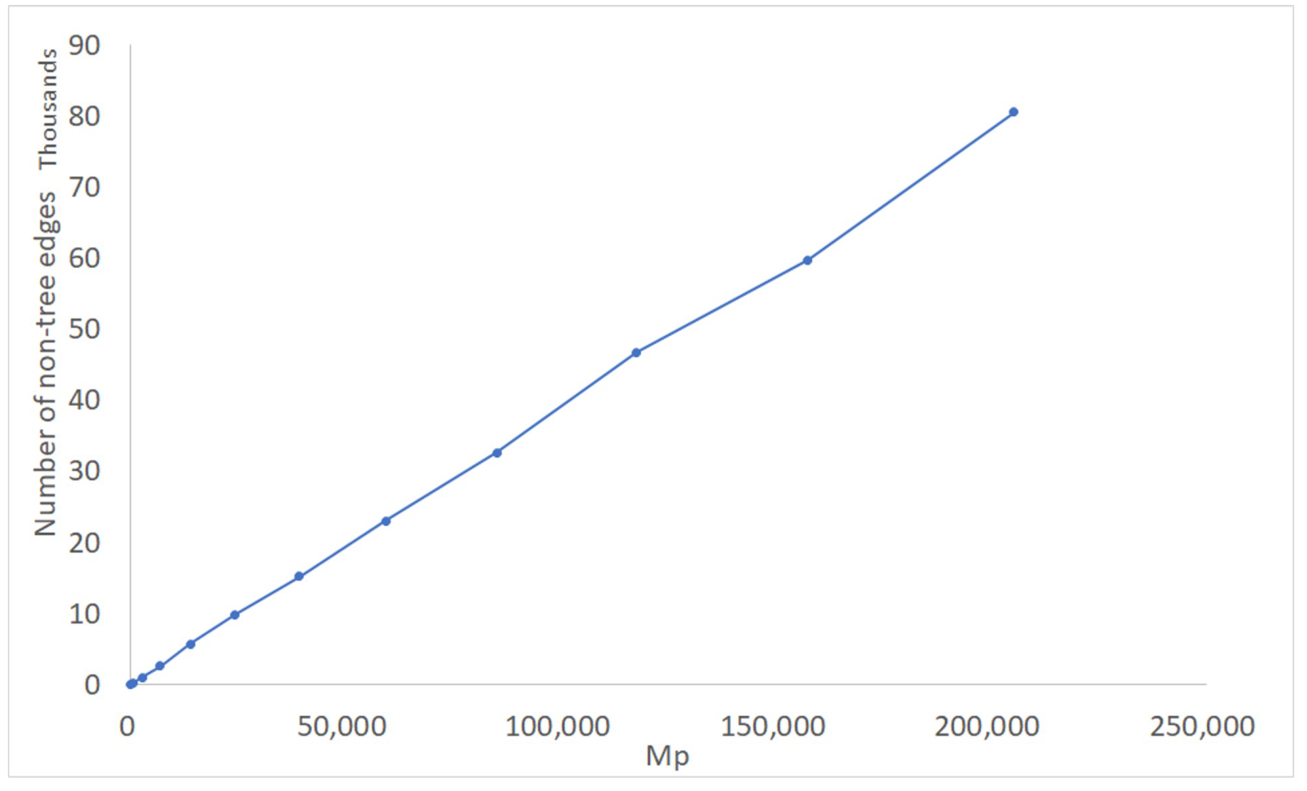
We now examine the impact of edge scans more closely. Figure 10 shows the average number of non-tree edges, as a function of $M_{\mathcal{P}}$, actually scanned by FCT(0) when operating on complete sets of rooted triples. Observe that not only does the number of edge scans increase at an only slightly super-linear rate, but also the average number of non-tree edges scanned is considerably smaller than $M_{\mathcal{P}}$. Together with Theorem 1, this explains the near-$\mathcal{O}(M_{\mathcal{P}}log{M}_{\mathcal{P}})$ behavior seen in Figure 7.

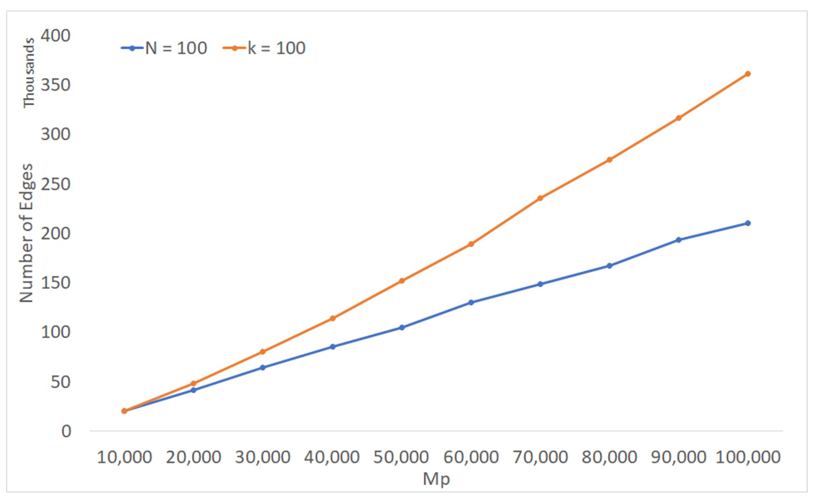
Figure 11 shows the average number of non-tree edges actually scanned by FCT(0) on profiles of binary phylogenies. The input profiles were generated as described in Section 5.4. As in that section, we varied one of n, the number of labels, or k, the number of trees, while keeping the other quantity fixed, and we took the product $n\times k$ as a proxy for $M_{\mathcal{P}}$.

When n was fixed, the number of non-tree edges scanned was roughly proportional to $M_{\mathcal{P}}$, suggesting that the running time of FCT(0) was $\mathcal{O}(M_{\mathcal{P}}log{M}_{\mathcal{P}})$. This is reflected in Figure 8a. On the other hand, when k was fixed, the number of non-tree edges scanned appeared to grow in a slightly super-linear manner. The explanation appears to be that increasing k increased the amount of overlap among the trees, and consequently also the number of non-tree edges. Nevertheless, the overall running time of FCT(0) in this case appeared close to $\mathcal{O}(M_{\mathcal{P}}log{M}_{\mathcal{P}})$; see Figure 8b. This may be because the effect of increasing the number of non-tree edges was mitigated by another factor: the sizes of the smaller of two subtrees resulting from edge deletion.

Table 11. Number of non-tree edges scanned by FPP(0) for matrices of order of 300 × 6000 with different density levels.

	5%	10%	15%	20%	25%	30%	35%	40%	45%	50%
Low	69,133	65,415	61,975	57,305	53,638	47,722	44,590	40,668	35,545	31,668
Medium	461,875	420,106	372,561	400,387	387,020	353,904	334,324	292,983	250,507	251,315
High	42,210	32,766	41,489	36,797	40,709	29,770	29,068	29,206	26,317	26,811

reports the number of non-tree edges scanned throughout the execution of FPP(0). Overall, the number of scanned non-tree edges was smaller than the total number of edges. This again illustrates that searching for replacement edges did not significantly contribute to the running time. Surprisingly, the largest number of edge scans occurred for medium-density matrices. We have not found a satisfactory explanation for this observation.

7.3. The Size of the Smaller Component

In the previous section, we saw that HDT(0) scanned relatively few non-tree edges when used in either FCT(0) or FPP(0).

Table 12. FCT(0): Number of subtrees of a size at most two versus number of subtrees of size greater than two for complete sets of triples.

${\mathit{M}}_{\mathcal{P}}$	65	730	2745	6860	13,825	24,390	39,305	59,320	85,185	117,650
Num. $\le 2$	29	355	1385	3498	7130	12,460	20,110	30,433	43,911	61,348
Num. $>2$	2	23	50	81	113	151	191	233	277	318

,

Table 13. FCT(0): Number of subtrees of a size at most two versus number of subtrees of size greater than two for profiles of binary trees with varying number of trees and 100 taxa.

${\mathit{M}}_{\mathcal{P}}$	10,000	20,000	30,000	40,000	50,000	60,000	70,000	80,000	90,000	100,000
Num. $\le 2$	7453	14,985	22,566	29,957	37,532	44,959	52,500	59,630	66,984	74,780
Num. $>2$	667	1156	1648	2104	2555	3201	3460	3966	4643	4975

,

Table 14. FCT(0): Number of subtrees of a size at most two versus number of subtrees of size greater than two for profiles of binary trees with varying number of taxa and 100 trees.

${\mathit{M}}_{\mathcal{P}}$	10,000	20,000	30,000	40,000	50,000	60,000	70,000	80,000	90,000	100,000
Num. $\le 2$	7473	15,098	22,711	30,403	37,903	45,636	53,083	60,638	68,336	75,946
Num. $>2$	683	1340	2037	2722	3387	4047	4759	5394	6017	6743

,

Table 15. FPP(0): Number of subtrees of a size at most two versus number of subtrees of size greater than two for medium-density matrices of order $300\times 6000$.

	5%	10%	15%	20%	25%	30%	35%	40%	45%	50%
Num. $\le 2$	27,592	27,793	26,951	27,358	27,358	27,126	26,711	26,839	26,590	26,003
Num. $>2$	924	926	940	972	969	983	983	976	976	979

and

Table 16. FPP(0): Number of subtrees of a size at most two versus number of subtrees of size greater than two for high-density matrices of order $300\times 6000$.

	5%	10%	15%	20%	25%	30%	35%	40%	45%	50%
Num. $\le 2$	31,130	30,709	31,054	30,443	30,194	29,359	29,393	28,839	27,603	26,696
Num. $>2$	882	908	905	907	901	908	892	912	900	879

show one reason for this: the smaller component was often very small. In fact, the small component often contained just one or two nodes. The tables show the number of times the smaller subtree resulting from an edge deletion had at most two nodes (“Num. $\le 2$”) and more than two nodes (“Num. $>2$”) for different types of input profiles. In all cases, subtrees of a size at most two outnumbered the rest by a wide margin.

Subtrees with at most two nodes (and, thus, one edge) were easily handled in $O(log{M}_{\mathcal{P}})$ time: the search for a replacement edge terminated immediately after encountering the first non-tree edge incident on one of the at most two nodes in the subtree, assuming such an edge exists.

Table 17. FCT(0): Number of subtrees of sizes $1,2,\cdots ,8$ and greater than 8 for profiles of binary trees with $k=100$ and varying n.

${\mathit{M}}_{\mathcal{P}}$	10,000	20,000	30,000	40,000	50,000	60,000	70,000	80,000	90,000	100,000
1	7012	14,188	21,324	28,550	35,603	42,883	49,848	56,924	64,181	71,334
2	461	910	1387	1853	2300	2753	3235	3714	4155	4612
3	158	287	434	586	721	862	1016	1154	1288	1448
4	88	157	239	315	393	472	560	615	689	794
5	56	101	149	197	242	290	350	392	431	495
6	38	70	102	137	166	197	238	266	294	348
7	27	48	71	101	125	143	174	190	218	245
8	20	37	54	78	95	113	132	151	167	182
>8	296	640	988	1308	1645	1970	2289	2626	2930	3231

examines the distribution of the size of the smaller component in greater detail for profiles of binary trees. The number of small components of a given size declined rapidly as the size increased. This pattern was evident even for profiles of trees of larger degrees, including for instances of IDPP, although it was somewhat less marked; see Tables S34–S46 of the Supplementary Materials. Invariably in our experiments, the overwhelming majority of the smaller subtrees had just one node. This means that, prior to deletion, the single node in that small component was a semi-universal node with just one incident tree edge.

8. Discussion

Our experimental results show that both the tree compatibility testing algorithm of [10] and the IDPP algorithm of [9] performed at least as well as their theoretical worst-case bounds, and often better, if implemented using HDT(0), a much-simplified version of the HDT dynamic connectivity data structure.

The results of Section 7 indicate that the main reason for the observed performance of HDT(0) is that the components that were scanned in search for replacement edges tended to be extremely small. Since we observed this phenomenon for a wide range of input profiles, we suspect that it is not an artifact of our experimental setup, but instead reflects a basic property of the graphs with which we are dealing. Indeed, $\mathtt{BuildNT}$ and $\mathtt{PPSS}$ use very special kinds of graphs—constructed from profiles of phylogenetic trees by gluing leaves with the same label—and perform deletions top-down. It is an open question whether there is a way to bound the total sizes of the smaller trees encountered during the execution of those algorithms, either asymptotically or in expectation.

Profiles consisting of binary trees—and, in particular, triples—are quite common in practice. Proposition 2(1b) of Section 7 implies that for such profiles, certain spanning forests are better than others for maintaining connectivity information. A “good” spanning forest is one where the number of semi-universal nodes incident to only one tree edge is large, relative to the total number of semi-universal nodes. The results reported in Section 7.3 (in particular, Table 17) indicate that the spanning forests our programs generated were good in this sense, despite the fact that the programs took no special measures to ensure this. It is an open question whether there is an analytical explanation for this phenomenon. Another open question is whether good spanning forests always exist and, if so, whether they can be constructed and maintained efficiently.

In our experiments, we never encountered a setting where HDT outperformed HDT(0). Of course, this does not mean that the latter is always to be preferred over the former. It would be interesting to find an application of dynamic graph connectivity where HDT is preferable to HDT(0) in practice.

References

- Steel, M.A. The complexity of reconstructing trees from qualitative characters and subtrees. J. Classif. 1992, 9, 91–116. [Google Scholar] [CrossRef]
- Semple, C.; Steel, M. Phylogenetics; Oxford Lecture Series in Mathematics; Oxford University Press: Oxford, UK, 2003. [Google Scholar]
- Chimani, M.; Rahmann, S.; Böcker, S. Exact ILP solutions for phylogenetic minimum flip problems. In Proceedings of the First ACM International Conference on Bioinformatics and Computational Biology, Niagara Falls, NY, USA, 2–4 August 2010; ACM: New York, NY, USA, 2010; pp. 147–153. [Google Scholar]
- Bininda-Emonds, O.R.P. (Ed.) Phylogenetic Supertrees: Combining Information to Reveal the Tree of Life; Series on Computational Biology; Springer: Berlin, Germany, 2004; Volume 4. [Google Scholar]
- Warnow, T. Supertree Construction: Opportunities and Challenges. arXiv, 2018; arXiv:1805.03530. [Google Scholar]
- Hinchliff, C.E.; Smith, S.A.; Allman, J.F.; Burleigh, J.G.; Chaudhary, R.; Coghill, L.M.; Crandall, K.A.; Deng, J.; Drew, B.T.; Gazis, R.; et al. Synthesis of phylogeny and taxonomy into a comprehensive tree of life. Proc. Natl. Acad. Sci. USA 2015, 112, 12764–12769. [Google Scholar] [CrossRef] [PubMed]
- Redelings, B.D.; Holder, M.T. A supertree pipeline for summarizing phylogenetic and taxonomic information for millions of species. PeerJ 2017, 5, e3058. [Google Scholar] [CrossRef] [PubMed]
- Aho, A.V.; Sagiv, Y.; Szymanski, T.G.; Ullman, J.D. Inferring a tree from lowest common ancestors with an application to the optimization of relational expressions. SIAM J. Comput. 1981, 10, 405–421. [Google Scholar] [CrossRef]
- Deng, Y.; Fernández-Baca, D. Fast compatibility testing for rooted phylogenetic trees. Algorithmica 2018, 80, 2453–2477. [Google Scholar] [CrossRef]
- Deng, Y.; Fernández-Baca, D. An efficient algorithm for testing the compatibility of phylogenies with nested taxa. Algorithms Mol. Biol. 2017, 12, 7. [Google Scholar] [CrossRef] [PubMed]
- Bryant, D.; Lagergren, J. Compatibility of unrooted phylogenetic trees is FPT. Theor. Comput. Sci. 2006, 351, 296–302. [Google Scholar] [CrossRef]
- Henzinger, M.R.; King, V.; Warnow, T. Constructing a tree from homeomorphic subtrees, with applications to computational evolutionary biology. Algorithmica 1999, 24, 1–13. [Google Scholar] [CrossRef]
- Pe’er, I.; Pupko, T.; Shamir, R.; Sharan, R. Incomplete directed perfect phylogeny. SIAM J. Comput. 2004, 33, 590–607. [Google Scholar] [CrossRef]
- Thorup, M. Decremental dynamic connectivity. J. Algorithms 1999, 33, 229–243. [Google Scholar] [CrossRef]
- Holm, J.; de Lichtenberg, K.; Thorup, M. Poly-logarithmic deterministic fully-dynamic algorithms for connectivity, minimum spanning tree, 2-edge, and biconnectivity. J. ACM 2001, 48, 723–760. [Google Scholar] [CrossRef]
- Nikaido, M.; Rooney, A.P.; Okada, N. Phylogenetic relationships among cetartiodactyls based on insertions of short and long interpersed elements: hippopotamuses are the closest extant relatives of whales. Proc. Natl. Acad. Sci. USA 1999, 96, 10261–10266. [Google Scholar] [CrossRef] [PubMed]
- Kimmel, G.; Shamir, R. The incomplete perfect phylogeny haplotype problem. J. Bioinform. Comput. Biol. 2005, 3, 359–384. [Google Scholar] [CrossRef] [PubMed]
- Even, S.; Shiloach, Y. An On-Line Edge-Deletion Problem. J. ACM 1981, 28, 1–4. [Google Scholar] [CrossRef]
- Henzinger, M.R.; King, V. Randomized fully dynamic graph algorithms with polylogarithmic time per operation. J. ACM 1999, 46, 502–516. [Google Scholar] [CrossRef]
- Thorup, M. Near-optimal fully-dynamic graph connectivity. In Proceedings of the 32nd Annual ACM Symposium on Theory of Computing, Portland, OR, USA, 21–23 May 2000; ACM: New York, NY, USA, 2000; pp. 343–350. [Google Scholar]
- Kapron, B.M.; King, V.; Mountjoy, B. Dynamic graph connectivity in polylogarithmic worst case time. In Proceedings of the Twenty-Fourth Annual ACM-SIAM Symposium on Discrete Algorithms, Society for Industrial and Applied Mathematics, New Orleans, LA, USA, 6–8 January 2013; pp. 1131–1142. [Google Scholar]
- Iyer, R.; Karger, D.; Rahul, H.; Thorup, M. An Experimental Study of Polylogarithmic, Fully Dynamic, Connectivity Algorithms. J. Exp. Algorithmics 2001, 6, 4. [Google Scholar] [CrossRef]
- Seidel, R.; Aragon, C.R. Randomized search trees. Algorithmica 1996, 16, 464–497. [Google Scholar] [CrossRef]
- Wojciechowski, M.; Sanderson, M.; Steele, K.; Liston, A. Molecular phylogeny of the “Temperate Herbaceous Tribes” of Papilionoid legumes: A supertree approach. In Advances in Legume Systematics; Herendeen, P., Bruneau, A., Eds.; Royal Botanic Gardens: Kew, UK, 2000; Volume 9, pp. 277–298. [Google Scholar]
- Kennedy, M.; Page, R.D.M. Seabird supertrees: Combining partial estimates of procellariiform phylogeny. Auk 2002, 119, 88–108. [Google Scholar] [CrossRef]
- Beck, R.M.D.; Bininda-Emonds, O.R.P.; Cardillo, M.; Liu, F.G.R.; Purvis, A. A higher-level MRP supertree of placental mammals. BMC Evol. Biol. 2006, 6, 93. [Google Scholar] [CrossRef] [PubMed]
- Prüfer, H. Neuer Beweis eines Satzes über Permutationen. Arch. Math. Phys. 1918, 27, 742–744. [Google Scholar]
- Pemmaraju, S.; Skiena, S. Computational Discrete Mathematics: Combinatorics and Graph Theory with Mathematica®; Cambridge University Press: Cambridge, UK, 2003. [Google Scholar]
Figure 1.
A profile. Leaves are labeled with species; internal nodes are numbered for later reference.
Figure 2.
A compatible supertree for the profile of Figure 1. Each internal node is labeled with the set of nodes that are mapped to it by the tree compatibility algorithm described in Section 4.1.
Figure 3.
The display graph for the profile of Figure 1.
Figure 4.
(Left) A character matrix A. (Right) The display graph for . The solid nodes and edges are the only part of the display graph that algorithm (Section 4.2) uses.
Figure 5.
The root position and its successor for the profile of Figure 1. Sets of nodes inside shaded boxes are positions. As a result of computing the successor, graph breaks down into two components. In this example, all nodes in the positions shown are semi-universal. Note, however, that, in general, not all nodes in a position are semi-universal (see [9,10]).
Figure 6.
Performance of FCT for varying degrees of level truncation on complete sets of triples.
Figure 7.
FCT(0) on profiles of rooted triples. (a) Complete sets of triples with varying number of taxa. (b) Rooted triples on 40 labels for different percentages of the maximum number of triples.
Figure 8.
FCT(0) on profiles of binary trees. (a) Running time for 100 trees and varying number of taxa. (b) Running time for 100 taxa and varying number of trees.
Figure 9.
Running time of FPP(0) and FPP(1) on matrices of order for (a) medium- and (b) high-density inputs.
Figure 10.
Number of non-tree edges scanned by FCT(0) for complete sets of rooted triples.
Figure 11.
Number of non-tree edge FCT scans for profiles of binary phylogenetic trees. The blue curve corresponds to varying k, while keeping n fixed at 100. The orange curve corresponds to varying n while keeping k fixed at 100.