Dissimilarity Space Based Multi-Source Cross-Project Defect Prediction

Abstract

Software defect prediction is an important means to guarantee software quality. Because there are no sufficient historical data within a project to train the classifier, cross-project defect prediction (CPDP) has been recognized as a fundamental approach. However, traditional defect prediction methods use feature attributes to represent samples, which cannot avoid negative transferring, may result in poor performance model in CPDP. This paper proposes a multi-source cross-project defect prediction method based on dissimilarity space (DM-CPDP). This method not only retains the original information, but also obtains the relationship with other objects. So it can enhances the discriminant ability of the sample attributes to the class label. This method firstly uses the density-based clustering method to construct the prototype set with the cluster center of samples in the target set. Then, the arc-cosine kernel is used to calculate the sample dissimilarities between the prototype set and the source domain or the target set to form the dissimilarity space. In this space, the training set is obtained with the earth mover’s distance (EMD) method. For the unlabeled samples converted from the target set, the k-Nearest Neighbor (KNN) algorithm is used to label those samples. Finally, the model is learned from training data based on TrAdaBoost method and used to predict new potential defects. The experimental results show that this approach has better performance than other traditional CPDP methods.

1. Introduction

The defect prediction model is helpful for software testers to allocate limited resources to the most error-prone software modules [1], which is important to the field of software quality assurance. Within-project defect prediction (WPDP) builds prediction models based on sufficient data from a software history store within the project, and these data satisfy the same statistical distribution. However, it is difficult to obtain sufficient training data in a new project, and as the company evolves, the previous data may no longer be applicable [2].

Cross-project defect prediction (CPDP) can solve the above problem in WPDP, and the method uses other project data to train prediction models, but due to the different development programming methods and other aspects of different projects, the distribution of source and target data sets are different [3]. Zimmermann et al. pointed out that the processing of data characteristics and processes is the key factor of CPDP method [1]. CPDP uses transferring learning methods to obtain useful information from the source domain that is similar to the distribution of the target data. This method can satisfy the same distribution hypothetical requirement between training and test data [4]. However, selecting source domain datasets randomly may result in negative transferring and poor performance because of low correlation with the target set [5]. The multi-source cross-project defect prediction method is proposed by researchers to reduce the effects of source component shift.

Experts have noticed that (dis)similarity representation can enhance the expression ability of samples, and the performance of classifier could be improved in pattern recognition [6,7]. The reason is that the dissimilarity is a crucial factor in recognition and categorization. By establishing the dissimilarity space, the original attributes of samples are replaced by the dissimilarity between pairs of samples. This method retains the original information of the dataset and makes each sample obtain the relationship with other objects, so it can enhance the discriminant ability of the sample attributes to the class label. The dissimilarity representation method maps samples into the dissimilarity space, in which several representative samples are selected from the target dataset as the prototype set. The samples of the dissimilarity space are calculated from the source domain, the target set and the prototype set. This method avoids the effects of different measurement standards for the same metric and reduces the dimension for classifiers [7]. How to build the training dataset in the dissimilarity space is critical to improving the performance of the prediction model.

In this paper, a multi-source cross-project defect prediction method based on dissimilarity space (DM-CPDP) is proposed. This DM-CPDP method has three phases. In the dissimilarity space constructing phase, we select some representative samples from the target set as the prototype set. Then, the arc-cosine kernel function is used to measure the sample dissimilarity between the prototype set and the source domain or target datasets. In the training dataset selection phase, the earth mover’s distance (EMD) method is used to calculate the cost, which is required to convert the data of the source domain, and in the dissimilarity space we select the corresponding samples with a small cost as the training set. In the last phase, we use the KNN method to assign labels to the unlabeled target samples, and the defect prediction model is constructed by the TrAdaBoost method in the dissimilarity space. The contributions to this paper can be highlighted as follows:

• In order to construct dissimilarity space, we propose a framework which uses the density-based clustering method to select all density center samples of the target set as the prototype set. Then the arc-cosine kernel function is utilized to measure the sample dissimilarity between the prototype set and the source domain or target datasets. The constructed dissimilarity space can represent the relationship between the multi-sources domain data and the target data.
• In order to construct the defect prediction model, we propose the DM-CPDP method. After constructing the dissimilarity space, this method uses the EMD method to select the samples in the dissimilarity space as the training dataset. For the unlabeled samples converted from the target set, the KNN algorithm is used to label those samples. TrAdaBoost method is utilized to establish the prediction model based on the selected training dataset. The DM-CPDP method avoids using the original feature space to construct the defect prediction model. In the traditional defect method, the defect prediction model makes multi-source domain data be fully utilized.
• To evaluate the performance of the DM-CPDP method, we compare it with other classic single-source and multi-source CPDP methods, such as TNB [8], TrAdaBoost [9], MsTrA [10], and HYDRA [11]. In addition, we compare the effects of several different dissimilarity measures and prototype selection methods. The necessity of multi-source data sets is also verified. In terms of performance metrics, we use F-measure, AUC (Area Under ROC Curve), and cost-effectiveness to measure the models performance. The experimental results show that the DM-CPDP method is much better than the other methods.

The remaining parts of this paper are as follows: This paper shows the related work in Section 2. The details of the DM-CPDP algorithm is described in Section 3. We verify the performance of the DM-CPDP method and analyze the experimental results in Section 4. The final part is the summary of this paper.

2. Related Work

Many researchers have stated in their papers that identifying defects in software as early as possible has great economic value [12]. Defect prediction is to establish a prediction model based on a software defect metric element in the early stage of defect detection. Traditional defect prediction is based on historical data within the project. Due to the difficulty of collecting the historical data, some new projects do not have historical data. Many researchers focus on cross-project defect prediction [9,12,13], and a series of classical CPDP methods are proposed. The key factor of CPDP is how to obtain the same distribution of data as the target set by transferring learning in the CPDP method. In order to realize positive transferring, the CPDP method based on multi-source dataset has attracted the attention of experts. In addition, Pekalska et al. [14] proposed that an appropriate representation of sample can improve the performance of the classifier, and it has been proved that classification prediction in dissimilarity spaces can achieve better results [15]. Therefore, this paper establishes the prediction model in the dissimilarity space.

2.1. Multi-Source CPDP

In recent years, multi-source CPDP methods are beginning to be considered to improve the performance of defect prediction [16,17]. Compared with a random selection of a single data set from the source domain as a training set, the multi-source CPDP method can avoid negative transferring, over-fitting problems, and make better performance of transfer learning [11]. Many researchers have proved that the multi-source cross-project software defect prediction can improve the performance of the prediction model and enhance generalization.

Yao and Doretto [13] proposed two multi-source CPDP methods: the first one is to establish multiple candidate weak classifiers according to the source domain data set in each iteration, and select the one with the lowest error rate as the weak classification of the current iteration; The second method is divided into two stages: firstly, all candidate weak classifications are obtained through multiple iterations, and then the classifier with the smallest error rate among the candidate weak classifiers is used as the current weak classifier in each iteration.

Yu et al. [10] proposed a multi-source TrAdaBoost (MsTrA) approach to construct prediction model. This method calculates the similarity between each candidate source data set sample and the target sample and gives weight to each sample at first. Then, on the basis of the TrAdaBoost algorithm, the classifier with the smallest error rate is selected as the weak classifier in each iteration, and the prediction model is obtained through multiple iterations.

Xia and David et al. [11] proposed HYDRA method, which constructs a multi-source CPDP model through two stages. In the first stage, they merge each candidate source and target dataset as the training set to construct multiple base-classifiers, then use the genetic algorithm (GA) to find the optimal combination of base-classifiers. The second phase is similar to the AdaBoost algorithm, and the GA model is generated in each iteration. Finally, a linear combination of GA models is obtained as a prediction model.

He et al. [18] based on the HYDRA method proposed the S³EL method that constructs basis classifier with feature mean values, and after that, GA is also used to assign weights to the basis classifier. Experiments show that those methods are superior to the conventional single-source CPDP methods.

The above methods provide important research approaches and ideas for multi-source CPDP research, but there are still some shortcomings. The MsTrA algorithm selects the optimal weak classifier in each iteration, which is prone to over-fitting problems. The HYDRA and S³EL method use the GA to search for the optimal weight combination of the classifiers in each iteration, thus the time complexity is higher. Therefore, this paper focus on solving the problems of data noise, generalization, and time complexity.

2.2. Dissimilarity Representation

Experts proposed using the pairwise dissimilarity between objects to represent the object and found that it can improve the performance of classifiers [19]. The traditional sample representation method uses feature attributes to represent a sample in the feature space. The disadvantage of this method is that the sample dimension is higher, and it is easy to cause the curse of dimensionality. The dissimilarity representation of samples can solve the problem, and the method represents a sample by calculating the dissimilarity relationship between the sample and the prototype set from the target set. The dimension of the sample is determined by the number of samples in the prototype set. Studies have shown that using the dissimilarity-based sample representation method can improve the performance of the defect prediction model. Compared with traditional modeling methods, this method can improve the performance by 1.86%–9.39% [20]. In addition, once the dissimilarity space has been constructed, many methods can be used to assign labels to unlabeled samples so that the model construction problem can be solved with a general standard supervised learning method [20].

The dissimilarity representation method mainly includes two factors: prototype set selection and dissimilarity transformation. The representation method uses a transformation function to map samples into dissimilarity spaces according to the prototype set. The dimensions of the space are determined by the number of samples contained in the prototype set, and the difference from the j-th prototype sample can be regarded as the j-th attribute in the space. Each attribute of each sample in the space is the dissimilarity between the sample and the prototype sample [7].

On the selection method of prototype set, there are many excellent methods, such as the nearest neighbor method, random selection method, and cluster-based linear programming method. The most conventional method uses random selection, but this method is uncertain and leads to information loss. Clustering algorithm can solve this problem, but the KNN usually needs to customize the k value, and cannot find all the representative samples. Alex and Alessandro [21] proposed a density peaks clustering (DPC) method which uses the density peak points of the data set to find the cluster center quickly. Therefore, this paper uses the DPC algorithm to select the representative sample as the prototype set.

In the problem of dissimilarity transformation, it is common to use a distance-based method to measure the relationship between samples and map the sample set into a $n\times m$ matrix, such as Euclidean distance, Mahalanobis distance, and Manhattan distance [15,19]. However, the accuracy will be affected if the measurement units are different for the above methods. For the cosine similarity, when the angle between vectors is the obtuse angle, these two vectors are irrelevant and the cosine value is negative. So the cosine similarity is not suitable for training the prediction model. The kernel method can describe the relationship between two vectors in essence, and it is more accurate than the distance-based method. Arc-cosine [22] is one of the kernel functions, and it represents the relationship between vectors by measuring the angle between vectors. Compared with cosine similarity measurement, this method is more intuitive in representing the relationship between vectors. Compared with radial basis function (RBF), this method does not need to adjust the parameters when only expressing the difference between vectors.

In order to improve the performance of the predictive model, the source domain dataset and the target set are used to construct the dissimilarity space, in which each sample is represented as the relationship between the source sample and the prototype set. The prototype set is obtained from the target set.

3. DM-CPDP Approach

Comparing with the traditional methods of building prediction models in the feature space, an alternative way is to construct prediction models in the dissimilarity space, in which each sample is described by pairwise dissimilarity relations between original data and the prototype set. In this paper, the kernel tool is used to measure the pairwise dissimilarity between candidate training data and prototype set, and then the data are mapped into the dissimilarity space. In the space, we achieve the transferring of multi-source datasets and assign labels to unlabeled target samples by a classification method, so that the process of model construction can use the standard supervised learning method. In order to offset the influence of useless features on the dissimilarity representation of samples, features need to be selected before the dissimilarity transformation. This paper chooses the FECAR [23] method for feature selection.

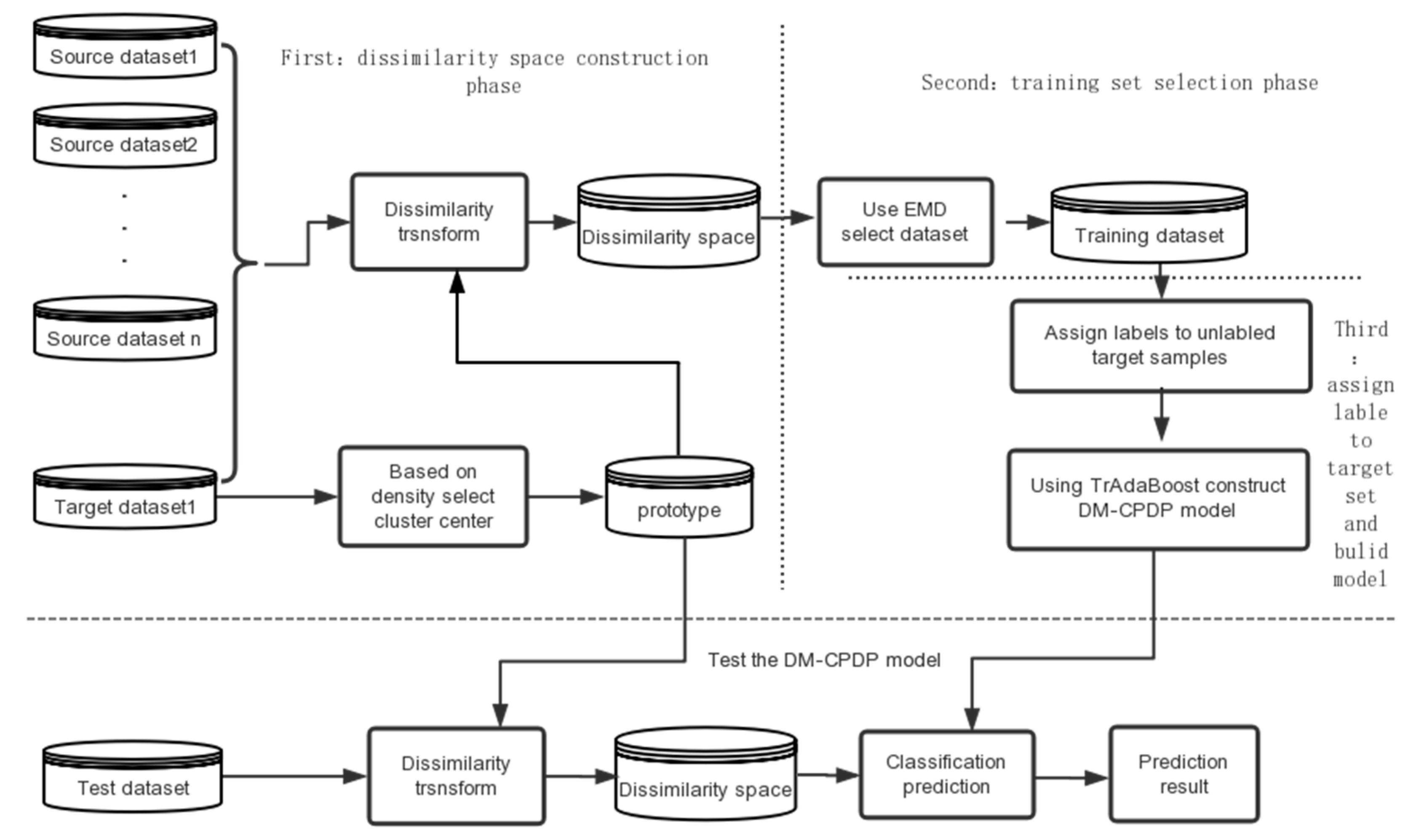
The overall process is shown in Figure 1. The process is divided into three phases. The first phase focus on constructing dissimilarity space. The density-based clustering method is used to calculate the cluster center of samples in the target set, and the prototype set is formed by those cluster center samples. Then, the arc-cosine kernel is used to calculate the sample dissimilarities between the prototype set and the source domain or the target set to form the dissimilarity space. In the second phase, the earth mover’s distance (EMD) method is used to calculate the cost, which is required to convert the data of the source domain, and in the dissimilarity space we select the corresponding samples with a small cost as the training set. In the third phase, the KNN method is used to assign labels to unlabeled target samples before building the prediction model, and then the TrAdaBoost method is used to construct the prediction model. In addition, the test set is also mapped into the dissimilarity space to obtain the predicted results.

3.1. Dissimilarity Space Construction

To construct a CPDP model in dissimilarity space, we represent the sample by the pairwise dissimilarity between the sample and the prototype set R obtained from the target set $X_T$. $R=\{p_1,p_2,\dots ,p_r\},R\in T$. In dissimilarity space, the set is represented as:

$$D\left(X,R=\left(p_1,p_2,\dots ,p_r\right)\right)={[k\left(x_i,p_j\right)]}_{n\times r}$$

(1)

Each instance is represented as a r-dimensional dissimilarity vector. $k(x_i,p_j)$ represents the dissimilarity between the i-th sample in data set X and the j-th prototype sample in prototype set R. This paper uses the density-based clustering method to select the cluster center as the prototype set, and uses the arc-cosine function to measure the pair-wise dissimilarity between samples.

3.1.1. Prototype Selection

To select the representative samples as the prototype from the target set, we use the clustering method to select the cluster center as the prototype sample to form the prototype set. Traditional clustering methods require defining the number of clusters artificially, and they cannot select all representative samples in the dataset. So we use the DPC method to cluster samples in this stage. The cluster center has two characteristics: high density and large distance. Cluster centers are surrounded by neighbors with lower local density and relatively large distances from other high-density points.

In the first step, we calculate the local density ${\rho }_i$ and local distance ${\delta }_i$ for each point.

The ${\rho }_i$ is equal to the number of points that are closer than $d_c$ to point i. The local density calculation method is as follows:

$${\rho }_i={\displaystyle \sum }_j\chi \left(d_{ij}-d_c\right)$$

(2)

The distance $d_{ij}$ between sample points is measured by Euclidean distance. $d_c$ is the cutoff distance which ensures each point has at least 2% of the total points as its neighbors, and $d_c>0$. Where $\chi (x)=1$ if $x<0$ and $\chi (x)=0$ otherwise.

The local distance calculation method is as follows:

$$\{\begin{array}{ll}{\delta }_i=\underset{j}{\max }(d_{ij}),& if{x}_{i}hasthe\max imum{\rho }_i\\ {\delta }_i=\underset{j:{\rho }_j>{\rho }_i}{\max }(d_{ij}),& otherwise\end{array}$$

(3)

The local distance has two cases: when the point $x_i$ with highest local density, ${\delta }_i$ is the greatest possible distance with others; otherwise, ${\delta }_i$ is the distance from $x_i$ to the nearest data point with greater local density.

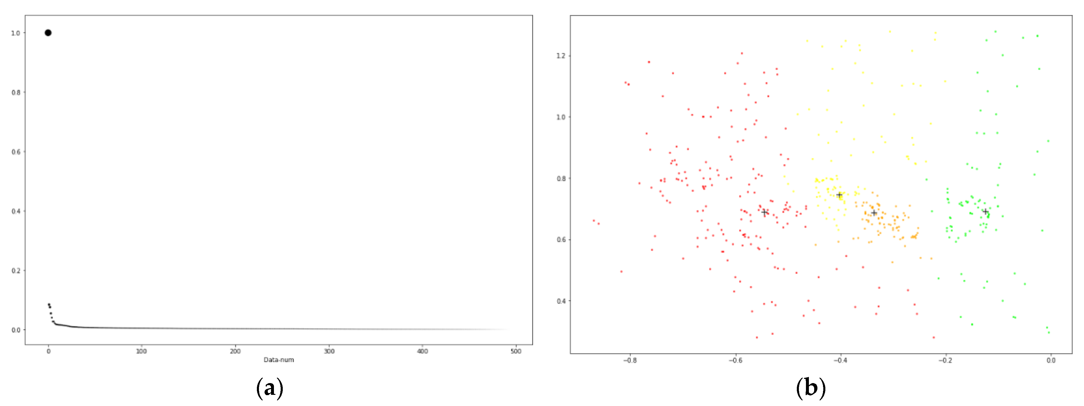
Then, the cluster center is selected by considering ${\delta }_i$ and ${\rho }_i$ in combination, and the method is shown in Formula (4). ${\delta }_i$ and ${\rho }_i$ maybe in different orders of magnitude, we normalize these two quantities, $z(·)$ is the normalized process. As shown in Figure 2, the points are sorted in descending order of ${\gamma }_i$ and represented in the form of a graph. The value of the non-cluster centers are relatively smooth and there is a clear jump from the non-cluster center to the cluster center. The points above the inflection point are chosen as the cluster centers.

$${\gamma }_i=z\left({\rho }_i\right)\times z\left({\delta }_i\right)$$

(4)

The method is shown in Algorithm 1. In step 3–7, we calculate the distance between samples, and sort the values of distance in ascending order. Then, the value of the 2%th data are selected as the cut-off distance $d_c$ in step 6–9. In step 10–14, the local density ${\rho }_i$ and local distance ${\delta }_i$ are calculated for each sample, and calculate the cluster center decision factor ${\gamma }_i$ according to ${\delta }_i$ and ${\rho }_i$. Last, we sort the value of ${\gamma }_i$ in descending order to select the cluster centers as the prototype set.

Algorithm 1. Prototype Selection
Input:   $X_T^{m\times k}$: data from the target set
Output:  the prototype $R^{r\times k}$
1	Initialize the current prototype $R\leftarrow \varphi$
	/*computer $d_{ij}$ and $d_c$ phase*/
2	$M=m(m-1)/2$ /*M is the number of $d_{ij}$, due to $d_{ij}=d_{ji},(i\ne j)$*/
3	for i = 1, 2, …, m do
4	for j = i + 1, i + 2, …, m do
5	Computer the distance $d_{ij}$ by the Euclidean distance
6	end
7	end
8	sort ${\left\{d_{ij}\right\}}_M$ in ascending order
9	$d_c\leftarrow (M\ast 0.02)th$ point distance value
	/*cluster center selection phase*/
10	for i = 1, 2, …, m do /*each sample $x_i$ belonging to $X_T^{m\times k}$*/
11	computer the density ${\rho }_i$ according to step 9 and Equation (2)
12	computer the distance ${\delta }_i$ according to Equation (3)
13	computer the candidate cluster center ${\gamma }_i$ as cluster center according to Equation (4)
14	end
15	Sort ${\left\{{\gamma }_i\right\}}_m$ in descending order
16	select all the cluster center as the prototype set R according to step15;
17	return $R^{r\times k}$

3.1.2. Dissimilarity Transformation

The novelty of this paper is to use a kernel function to interpret the dissimilarity between samples in dissimilarity spaces. The kernel tools can represent a certain relationship between two objects. When relaxing the requirement for Mercer kernels, there are more powerful dissimilarity measures can be defined in the domain [24]. With the goal of better representing the dissimilarity between vectors, the arc-cosine kernel is used to measure the dissimilarity between samples. According to the analysis of the arc-cosine kernel, we use $k_0(x,y)$ to measure the pair-wise dissimilarity, short in $k(x,y)$, and shown as:

$$k\left(x,y\right)=1-\frac{1}{\pi }{\cos }^{-1}\frac{x·y}{\left|\left|x\right|\right|·\left|\left|y\right|\right|}$$

(5)

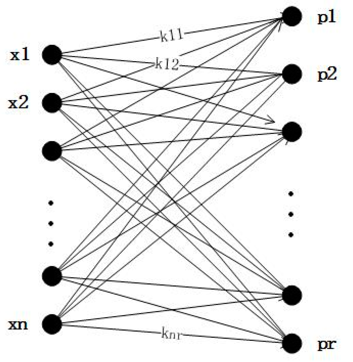
In the transformation process, we first use the arc-cosine kernel function to measure the dissimilarity between each original sample and the prototype set, and these values are used as row vectors, and then the low-dimensional dissimilarity space is constructed. The process is shown in Figure 3 and Equation (6). The dimension of this space is determined by the number of samples in the prototype set R. $k(x_i,p_j)$ represents the dissimilarity between the sample $x_i$ and the prototype sample $p_j$.

$$D(X,R)\stackrel{\Delta }{=}\left(\begin{array}{l}{x}_1^{\prime }\\ x_2^{\prime }\\ ⋮\\ x_n^{\prime }\end{array}\right)=\left(\begin{array}{ccccc}{p}_1& p_2& \cdots & p_r& Class\\ x_{1}k(x_1,p_1)& k(x_1,p_2)& \cdots & k(x_1,p_r)& y_1\\ x_{2}k(x_2,p_1)& k(x_2,p_2)& \cdots & k(x_2,p_r)& y_2\\ ⋮& & & ⋮& ⋮\\ x_{n}k(x_n,p_1)& k(x_n,p_2)& \cdots & k(x_n,p_r)& y_n\end{array}\right)$$

(6)

Each sample in the dissimilarity space is represented as:

$$x_i^{\prime }=k\left(x_i,R\right)=\left\{k\left(x_i,p_1\right),k\left(x_i,p_2\right),\dots ,k\left(x_i,p_r\right)\right\}$$

(7)

Algorithm 2. Dissimilarity Space Construction
Input:   $X_S^{n\times k}$: data from the source domain data set
$X_T^{m\times k}$: data from the target set
$R^{r\times k}$: the data of prototype, $R\in X_T^{m\times k}$
u: the number of source domain data set
Output:  D: dissimilarity space
1	initialize the current $D\leftarrow \varphi$
	/*map source domain data sets into D*/
2	for each $X_{Su}^{n\times k}\in S$ do
3	initialize the current $D(X_{Su},R)\leftarrow \varphi$
4	for each $x_i\in X_{Su}^{n\times K}$ do
5	for each $p_j\in R^{r\times k}$ do
6	computer $k(x_i,p_j)$ according to Equation (5)
7	end
8	get another representation of sample $x_i$: $x_i^{\prime }$
9	$D(X_{Su},R)\leftarrow D(X_{Su},R)\cup x_i^{\prime }$
10	end
11	$D\leftarrow D\cup D(X_{Su},R)$
12	end
	/*map target data set to D*/
13	for each $x_i\in X_T^{m\times K}$ do
14	initialize the current $D(X_T,R)\leftarrow \varphi$
15	repeat step 5–8
16	$D(X_T,R)\leftarrow D(X_T,R)\cup x_i^{\prime }$
17	end
18	$D\leftarrow D\cup D(X_T,R)$
19	Return D

The above methods are used to map each source domain and target dataset into the dissimilarity space. The dissimilarity space construction method is shown in Algorithm 2. Step 3–9 is the process of mapping a source domain data set into the subspace. In this stage, $x_i^{\prime }$ is the dissimilarity representation of the sample $x_i$. It is obtained by calculating the dissimilarity between each source data sample and the prototype set. Then we add $x_i^{\prime }$ to the subspace $D(X_{Su},R)$. Step 13–17 is the process of mapping target set into dissimilarity, and the process is similar to the source domain dataset. Finally, the dissimilarity space D is obtained by combining these subspaces.

3.2. Selection of Multi-Source Datasets

To select the appropriate data sets, the earth mover’s distance (EMD) is used to measure the similarity between the sets. The EMD is defined as the minimum amount of work that required to convert a data distribution to another, i.e., assuming X is a warehouse containing n mound and R is a warehouse with p empty pits. The similarity between datasets is the minimal cost to move n mound in X to p pits in R.

In this stage, the dataset can be represented as $X=\{(x_1,w_{x_1}),\dots ,(x_i,w_{x_i}),\dots ,(x_n,w_{x_n})\}$. $w_{xi}$ is the weight of $x_i$. When using the EMD method, we assume each sample $x_i$ is a mound with the quality $w_{xi}$. Similarly, the prototype set is represented as $R=\{(p_1,w_{p_1}),\dots ,(p_j,w_{p_j}),\dots ,(p_r,w_{p_r})\}$. $w_{pj}$ is the weight of $p_j$. In the EMD method, we assume each sample $p_j$ is an empty pit with the volume of $w_{pj}$.

We consider that the quality of each sample in the same set is equal and the total mass is equal to the total capacity, and the conditions are shown in (8). $d_{ij}$ is the cost of moving $x_i$ to $p_j$, and the calculation method as shown in (9). $k(x_i,p_j)$ comes from the matrix (7). We consider the cost function $D_{XR}$ from X to R as the similarity between the source data set and the prototype set, that is, the similarity between the source data set and the target set. The cost function $D_{XR}$ refers to the Equation (10).

$$\{\begin{array}{l}{w}_{x_i}=\frac{1}{n}\\ w_{p_j}=\frac{1}{r}\\ {\displaystyle {\displaystyle \sum }_{i=1}^n}{w}_{x_i}={\displaystyle {\displaystyle \sum }_{j=1}^r}{w}_{p_j}=1\end{array}$$

(8)

$$d_{ij}=1-k\left(x_i,p_j\right)$$

(9)

$$D_{XR}=min{\displaystyle \sum }_{i=1}^n{\displaystyle \sum }_{j=1}^r{d}_{ij}{f}_{ij}$$

(10)

$f_{ij}$ defines the flow from $x_i$ to $p_j$. The method aims to find an optimal solution $\left\{f_{ij}\right\}$ to minimize the overall cost function, and it is subjected to the following constraints:

$$\{\begin{array}{l}{f}_{ij}\ge 0,1\le i\le n;1\le j\le r\\ {\displaystyle \sum _{j=1}^r{f}_{ij}=w_{x_i},1\le i\le n}\\ {\displaystyle \sum _{i=1}^n{f}_{ij}=w_{p_j},1\le j\le r}\\ {\displaystyle \sum _{i=1}^n{\displaystyle \sum _{j=1}^r{f}_{ij}}=\min \{{\displaystyle \sum _{i=1}^n{w}_{x_i}},{\displaystyle \sum _{j=1}^r{w}_{p_j}}\}}\end{array}$$

(11)

The method of data set selection is shown in Algorithm 3. In step 2–6, we calculate the cost function of converting the source domain data set into the same data distribution as the prototype set. In step 8–10, the values of cost function $D(X_{Su},R)$ are sorted in descending order, and the first α datasets are selected as the training set.

Algorithm 3. Selection of multi-source datasets
Input:  $D(X_{Su},R)$: representation of source domain data set $X_{Su}$ in space D
u: the number of source domain data set in space D
Output:  training dataset
1	for each $D{(X_{Su},R)}^{n\times r}$ in D
2		for each $x_i^{\prime }$ in $D(X_{Su},R)$ do
3		computer the move cost $d_{ij}$ according to Equation (9)
4		computer the optimum solution $\left\{f_{ij}\right\}$ according to Equation (8) and the restrictions of Equation (11)
5		computer the cost function $D_{X_{Su}R}$ according to Equation (10)
6		end
7	end
8	sort ${\left\{D_{X_{Su}R}\right\}}_u$ in descending order
9	select the first α dataset as the training dataset
10	return training dataset

3.3. Model Construction

Since the values of all sample attributes are in [0, 1] after dissimilarity transformation, the KNN method can be used without being affected by noise in the dissimilarity space. Each attribute of the sample represents the degree of dissimilarity between the original sample and the prototype sample in the dissimilarity space, and the more similar to the prototype, the greater the value we get. So that the KNN method is suitable for assigning labels in the space. This method finds k points closest to the target sample. Then, the voting method is used to assign a label to the target sample, and the voting method is calculated by the Equation (12). Therefore, statistical-based machine learning algorithms can be used to build prediction models. In order to achieve better transferring, we use the classic TrAdaBoost algorithm to build the prediction model.

$$y=sign({\displaystyle \sum }_{i=1}^{k}I\left(y_i=+1\right)-{\displaystyle \sum }_{i=1}^{k}I\left(y_i=-1\right))$$

(12)

$I(·)$ is the number of samples marked as positive (negative) in k samples. $sign(x)$ is a symbolic function, where $sign(x)=1$ if $x\ge 0$ and $sign(x)=0$ otherwise.

4. Experiments

4.1. DataSet

In order to verify the effectiveness of the DM-CPDP method, we validate the performance of the prediction model through experiments and compare it with other methods. In this paper, we selected 14 datasets in NASA and 3 datasets in SOFTLAB to experiment. The datasets of NASA and SOFTLAB are obtained from PROMISE repository. The PROMISE repository is constantly updating datasets. Compared to the datasets used in some of the previous papers [8,12], the current datasets have some variation in the number of samples, but its internal structure has not changed to some extent. Since this paper constructing cross-project software defect prediction model based on multi-source datasets, the impact of some change in the number of samples on the experimental results is limited. To facilitate comparison with previous studies, we used previous versions of datasets maintained by the PROMISE repository. These datasets are shown in

Table 1. Data set.

Project	Examples	Defect Class	%Defective	Features
NASA
CM1	327	42	12.84	37
PC1	705	61	8.65	37
PC2	745	16	2.15	36
PC3	1563	160	10.24	37
PC4	1287	177	13.75	37
PC5	1723	471	27.34	39
KC1	1183	314	26.54	21
KC2	522	107	20.49	21
KC3	194	36	18.56	39
KC4	125	61	48.80	42
MC1	327	42	12.84	37
MC2	125	55	35.20	39
MW1	253	27	10.67	37
JM1	10878	2105	19.35	21
SOFTLAB
ar3	63	8	12.70	29
ar4	107	20	18.69	29
ar5	36	8	22.22	29

.

These datasets are derived from different projects, and the data distribution as well as feature attributes are different. We choose the common attributes of the target set and the source domain dataset to build the prediction models.

Table 2. Software metric element.

Metrics	Type	Metric	Type
UniqOpnd	DHalstead	LOC	McCabe
TotalOp	DHalstead	EV(g)	McCabe
UniqOp	DHalstead	V(g)	McCabe
TotalOpnd	DHalstead	IV(g)	McCabe
L	DHalstead	LOCcode	LineCount
V	DHalstead	LOCComment	LineCount
N	DHalstead	LOCBlank	LineCount
I	DHalstead	LOCCodeAndcomment	LineCount
D	DHalstead	B	DHalstead
T	DHalstead	E	DHalstead

shows the metrics of the software features used in the experiment. It mainly includes McCabe metric element, Line Countmetric element, Halstead basic metric element, and its extension DHalstead metric element.

To facilitate comparison, we performed two parts of the experiment on the data sets: NASA to NASA, NASA to SOFTLAB.

NASA to NASA: Only the NASA is used as the target set and the training set. Each dataset belonging to the NASA is chosen as the target set, and the remaining data sets are used as the training set.

NASA to SOFTLAB: All datasets belonging to NASA are used as source domain datasets, and datasets in SOFTLAB are used as the target sets.

4.2. Performance Index

In this paper, the prediction results are measured according to the indexes of F-measure, AUC (Area Under ROC Curve), and cost-effectiveness. The performance index is calculated based on the confusion matrix shown in

Table 3. Confusion Matrix.

	Predicted Positive	Predicted Negative
Real positive	TP	FN
Real negative	FP	TN

.

True Positive (TP): represents the number of positive samples predicted as positive classes.

False Positive (FP): represents the number of positive samples predicted as negative classes.

False Negative (FN): represents the number of negative samples predicted as positive clasess.

True Negative (TN): represents the number of negative samples predicted as negative classes.

F-measure is determined by both recall and precision, and its value is close to the smaller value of both. So that the larger F-measure means that both recall and precision are larger, the formula is shown in (13), where α is used to regulate the relative importance of precision and recall, and its value is usually at 1.

$$\mathrm{F}\text{-}\mathrm{measure}=\frac{\left(1+\alpha \right)\times \mathrm{recall}\times \mathrm{precision}}{\mathrm{recall}+\alpha \ast \mathrm{precision}}$$

(13)

$$\mathrm{recall}=\frac{\mathrm{TP}}{\mathrm{TP}+\mathrm{FN}}$$

(14)

$$\mathrm{precision}=\frac{\mathrm{TP}}{\mathrm{TP}+\mathrm{FP}}$$

(15)

Recall is the ratio of correctly predicting the number of defective modules to the number of real defective modules, indicating how many positive samples are correctly predicted.

Precision is the ratio between correctly predicting the number of defective modules and the number of all predicted defective modules, indicating how many predictions are correct in positive samples.

AUC is defined as the area under the receiver operating characteristics (ROC) curve. This performance indicator is one of the criteria for judging the two-category model.

Cost-effectiveness refers to maximizing benefits by spending the same cost. Cost-effectiveness measures the percentage of defects that can be identified by the predictive model by examining the top 20 percent of the samples [11,25]. Zhang et al. consider that the cost of software includes not only the effort of inspecting the defective modules, but also the failure cost of classifying a defective sample as a non-defective sample [26]. Incorrectly predicted defective samples will have a greater impact on software. Therefore, they propose a measurement method based on confusion matrix, and the cost-effectiveness is calculated according to the Equation (16). Compared with other methods, this method is more concise, and it is not affected by the order and the size of defect modules. The smaller the value means the lower the false negative of the prediction result of the model, and the more defective modules can be correctly predicted. So, the cost of failure caused by the software in the later stage is being lower.

$$\mathrm{cost}\text{-}\mathrm{effectiveness}=\frac{\mathrm{FN}}{\mathrm{FN}+\mathrm{TN}}$$

(16)

4.3. Analysis of Results

By comparing with traditional single-source and multi-source defect prediction methods, we prove that establishing prediction models in the dissimilarity space can improve the performance of the prediction model, and prove the superiority of the DM-CPDP method. The construction of classifier in the dissimilarity space is mainly influenced by two factors: dissimilarity metric and prototype selection. We compared the effects of different dissimilarity metric and prototype selection methods on the experimental results. In addition, the necessity of multi-source data in CPDP is also be verified.

4.3.1. Experiment on Different Methods

In order to verify the superiority of the DM-CPDP method, we compare it with traditional CPDP models.

In this part, we conduct experiments on NASA to NASA and NASA to SOFTLAB respectively. Among many traditional CPDP methods, this paper chooses three classical comparison methods, such as TNB, MSTrA, and HYDRA method. In each experiment, 90% of the source data set and target set are selected randomly as the training set, and the data of remaining target set are used as the test set. Each experiment was repeated 10 times, and the average values of these experiments are obtained from the results. The experimental details of each method are as follows:

TNB: randomly selects a dataset as the training set, and assigns weights to the training samples according to the target set using data gravity. Finally, the defect prediction model is built using the NB algorithm.

MSTrA: selects multiple data sets as training set and distributes weights for each training data according to the target set using data gravitation. In each iteration, each source domain data set is matched with the target set to train weak classifiers, and the weak classifier in the current iteration with the lowest error rate on the target set is selected.

HYDRA: merges each candidate source and target dataset as the training set to construct multiple base-classifiers, and then use the genetic algorithm to find the optimal combination of base-classifiers. After that, the process which is similar to the AdaBoost algorithm is used to obtain a linear combination of GA models.

The results are shown in

Table 4. Comparison of performance indicators F-measure.

Target Set	TNB	MSTrA	HYDRA	DM-CPDP
NASA to NASA
CM1	0.293	0.562	0.665	0.594
PC1	0.159	0.455	0.409	0.635
PC2	0.237	0.172	0.293	0.368
PC3	0.204	0.464	0.801	0.776
PC4	0.198	0.352	0.490	0.468
PC5	0.323	0.517	0.607	0.647
KC1	0.467	0.585	0.769	0.832
KC2	0.566	0.571	0.905	0.684
KC3	0.258	0.537	0.454	0.450
KC4	0.307	0.273	0.479	0.502
MC1	0.332	0.446	0.681	0.755
MC2	0.527	0.409	0.514	0.597
MW1	0.213	0.282	0.227	0.393
JM1	0.396	0.563	0.595	0.811
average	0.320	0.442	0.564	0.608
NASA to SOFTLAB
ar3	0.416	0.708	0.755	0.781
ar4	0.509	0.714	0.713	0.753
ar5	0.652	0.809	0.846	0.863
average	0.526	0.743	0.771	0.799

,

Table 5. Comparison of performance indicators AUC.

Target Set	TNB	MSTrA	HYDRA	DM-CPDP
NASA to NASA
CM1	0.642	0.674	0.793	0.782
PC1	0.584	0.596	0.624	0.810
PC2	0.557	0.535	0.576	0.563
PC3	0.629	0.686	0.879	0.842
PC4	0.577	0.710	0.696	0.735
PC5	0.741	0.643	0.662	0.768
KC1	0.632	0.722	0.818	0.892
KC2	0.776	0.813	0.857	0.853
KC3	0.733	0.565	0.689	0.685
KC4	0.658	0.581	0.756	0.793
MC1	0.497	0.664	0.781	0.836
MC2	0.630	0.609	0.659	0.662
MW1	0.681	0.657	0.495	0.715
JM1	0.629	0.708	0.729	0.839
average	0.640	0.656	0.715	0.770
NASA to SOFTLAB
ar3	0.719	0.726	0.786	0.790
ar4	0.738	0.715	0.811	0.837
ar5	0.831	0.836	0.864	0.885
average	0.762	0.759	0.820	0.837

and

Table 6. Comparison of performance indicators cost-effectiveness.

Target Set	TNB	MSTrA	HYDRA	DM-CPDP
NASA to NASA
CM1	0.089	0.047	0.041	0.039
PC1	0.071	0.035	0.039	0.027
PC2	0.002	0.002	0.001	0.001
PC3	0.083	0.056	0.019	0.022
PC4	0.114	0.087	0.058	0.061
PC5	0.172	0.103	0.069	0.057
KC1	0.126	0.097	0.053	0.047
KC2	0.075	0.074	0.039	0.035
KC3	0.147	0.079	0.072	0.084
KC4	0.204	0.265	0.185	0.142
MC1	0.087	0.068	0.040	0.039
MC2	0.113	0.152	0.144	0.119
MW1	0.084	0.089	0.083	0.076
JM1	0.096	0.074	0.074	0.036
average	0.105	0.088	0.066	0.056
NASA to SOFTLAB
ar3	0.062	0.045	0.041	0.040
ar4	0.057	0.046	0.046	0.042
ar5	0.049	0.034	0.032	0.031
average	0.056	0.042	0.040	0.038

, bold numbers indicate optimal results on a dataset.

It can be seen that the DM-CPDP method outperforms several existing algorithms on most data sets. In the NASA to SOFTLAB experiments, the performance of each algorithm on SOFTLAB data sets is stable. DM-CPDP method is better than the other algorithms. The average value of F-measure and AUC are 2.8%–27.3% and 1.7%–7.8% respectively, which is higher than other algorithm. In addition, the average value of the cost-effectiveness for the DM-CPDP method is 1%–4.9%, which is lower than other algorithms.

In the NASA to NASA experiment, the average value of DM-CPDP method on F-measure and AUC are higher than other methods: 4.4%–28.8%, 5.5%–13.0% respectively. The average value of DM-CPDP method on cost-effectiveness is lower than other methods 0.2%–1.8%. For the three metrics of F-measure, AUC, and cost-effectiveness, they are 9, 9, and 10 datasets respectively showing the best performance on the DM-CPDP method. For the HYDRA, there are 4, 4, and 3 datasets respectively showing the best performance. For the MSTrA method, only one dataset shows the best performance on the F-measure indicator. For the TNB method, there is one dataset performs optimally on AUC and cost-effectiveness respectively.

The reason for the above phenomenon is the influence of data distribution. Different machine learning methods behave different on the same data set, and the same machine learning method performs differently on different datasets. DM-CPDP is still superior to other algorithms in general. The reason is that this method uses multi-source datasets and dissimilarity representation method. By comparing with these three classic CPDP methods, it can be proved that DM-CPDP method performs well in the field of CPDP.

4.3.2. Experiments on Multi-Source Data Sets and Dissimilarity Space

In order to verify the impact of multi-source data and sample dissimilarity representation on the performance of predictive models, we compare the TrAdaBoost, Multi-source TrAdaBoost, dissimilarity space based single-source CPDP (DS-CPDP) method, and DM-CPDP method. All the comparisons base on F-measure, AUC, and cost-effectiveness to complete. Each experiment was repeated 10 times, and the average values of these experiments are obtained from the results. The experimental details of each method are as follows:

TrAdaBoost: randomly selects 90% of the source domain data set and target set as the training set, and the remaining target set as the test set. The prediction model was built using TrAdaBoost.

Multi-source TrAdaBoost: before using the TrAdaBoost algorithm to build a prediction model, the EMD method is used to select multiple data sets that are highly correlated with the target set, then these data sets are combined with the target set as a training set. Finally, the TrAdaBoost algorithm is used for modeling.

DS-CPDP: randomly selects a data set from the source domain for dissimilarity transformation as the training set, and then uses KNN method to assign labels to unlabeled target, after that use the TrAdaBoost method to build the model.

The experimental results are shown in

Table 7. F-measure value of different model construction methods. DS-CPDP: dissimilarity space based single-source CPDP.

Target Set	TrAdaBoost	Multi-Source TrAdaBoost	DS-CPDP	DM-CPDP
NASA to NASA
CM1	0.419	0.525	0.564	0.594
PC1	0.364	0.412	0.538	0.635
PC2	0.259	0.160	0.295	0.368
PC3	0.578	0.601	0.698	0.776
PC4	0.239	0.237	0.316	0.468
PC5	0.485	0.493	0.601	0.647
KC1	0.534	0.556	0.788	0.832
KC2	0.471	0.514	0.652	0.684
KC3	0.268	0.315	0.400	0.450
KC4	0.427	0.462	0.454	0.502
MC1	0.620	0.629	0.687	0.755
MC2	0.395	0.408	0.521	0.597
MW1	0.169	0.201	0.385	0.393
JM1	0.535	0.549	0.718	0.811
average	0.412	0.433	0.544	0.608
NASA to SOFTLAB
ar3	0.586	0.705	0.739	0.781
ar4	0.577	0.691	0.724	0.753
ar5	0.795	0.829	0.837	0.863
average	0.653	0.742	0.767	0.799

,

Table 8. AUC value of different model construction methods.

Target Set	TrAdaBoost	Multi-Source TrAdaBoost	DS-CPDP	DM-CPDP
NASA to NASA
CM1	0.639	0.662	0.716	0.782
PC1	0.592	0.601	0.723	0.810
PC2	0.519	0.532	0.531	0.563
PC3	0.640	0.669	0.715	0.842
PC4	0.568	0.689	0.683	0.735
PC5	0.625	0.631	0.725	0.768
KC1	0.711	0.724	0.841	0.892
KC2	0.797	0.806	0.819	0.853
KC3	0.518	0.574	0.596	0.685
KC4	0.570	0.577	0.628	0.793
MC1	0.633	0.654	0.746	0.836
MC2	0.549	0.593	0.615	0.662
MW1	0.627	0.651	0.684	0.715
JM1	0.665	0.701	0.782	0.839
average	0.618	0.641	0.700	0.770
NASA to SOFTLAB
ar3	0.684	0.734	0.752	0.790
ar4	0.629	0.714	0.741	0.837
ar5	0.717	0.810	0.856	0.885
average	0.677	0.753	0.783	0.837

and

Table 9. Cost-effectiveness value of different model construction methods.

Target Set	TrAdaBoost	Multi-Source TrAdaBoost	DS-CPDP	DM-CPDP
NASA to NASA
CM1	0.071	0.057	0.054	0.039
PC1	0.404	0.068	0.032	0.027
PC2	0.002	0.001	0.001	0.001
PC3	0.069	0.059	0.047	0.022
PC4	0.093	0.082	0.066	0.061
PC5	0.124	0.111	0.078	0.057
KC1	0.114	0.108	0.059	0.047
KC2	0.086	0.068	0.033	0.035
KC3	0.106	0.092	0.087	0.084
KC4	0.250	0.234	0.176	0.142
MC1	0.051	0.049	0.044	0.039
MC2	0.188	0.174	0.136	0.119
MW1	0.094	0.091	0.082	0.076
JM1	0.077	0.052	0.046	0.036
average	0.124	0.089	0.067	0.056
NASA to SOFTLAB
ar3	0.057	0.052	0.044	0.040
ar4	0.060	0.049	0.045	0.042
ar5	0.047	0.039	0.038	0.031
average	0.055	0.047	0.042	0.038

, bold numbers indicate optimal results on a dataset.

In order to prove the importance of multi-source data, we verify it in the dissimilarity space and the feature space respectively. By comparing the results of DM-CPDP and DS-CPDP method, it can be found that DM-CPDP is superior to DS-CPDP in the three indexes of F-measure, AUC, and cost-effectiveness in the dissimilarity space. The average value of F-measure is higher than the DS-CPDP method by 6.4% and 3.2% in the two series of datasets respectively. The average value of AUC is higher than the DS-CPDP method by 7.0% and 5.4%. The average value of cost-effectiveness is lower than the DS-CPDP method by 1.1% and 0.4%. By comparing the results of TrAdaBoost and Multi-source TrAdaBoost, it can be found that the Multi-source TrAdaBoost method is better than the TrAdaBoost in the feature space, and the average value of F-measure is higher than the TrAdaBoost method by 2.1%, 8.9%. The average value of AUC is higher than the TrAdaBoost method by 2.3%, 7.6%. The average value of cost-effectiveness is lower than the TrAdaBoost method by 3.5%, 0.8%. These results prove that the CPDP method based on multi-source data can improve the performance of prediction models, whether in the dissimilarity space or in the feature space.

The reason why multi-source data is superior to single-source data is that multi-source method in CPDP can not only increase the useful information by providing sufficient data, but also effectively avoid the problem of negative transferring. Besides, in the process of modeling, we also filter the multi-source datasets and select the data highly correlated with the target set as the training set. So that the data distribution of the training set and the target set is as similar as possible. Thus, multi-source data can improve the predictive performance of classifiers.

In order to verify that the construction of dissimilarity space can improve the performance of the classifier, these two sets of experiments are compared: TrAdaBoost and DS-CPDP, Multi-source TrAdaBoost and DM-CPDP. From the experimental results in Table 7, Table 8 and Table 9, the average value of F-measure on DS-CPDP is 13.2% and 11.4% respectively, which is higher than the TrAdaBoost algorithm. The average value on AUC is higher than the latter by 8.2%, 10.6%. The average value on cost-effectiveness is lower than the latter by 5.7%, 1.3%. By comparing DM-CPDP with Multi-source TrAdaBoost, we can find that the former is better than the latter in the average value of the two performance indicators. The average value of F-measure in the former is higher than that in the latter 17.5% and 5.7% respectively. In terms of AUC, the former is better than the latter 12.9% and 8.4% respectively. The average value on cost-effectiveness is lower than the latter by 3.3%, 0.9%. Therefore, it can be proved that the model established in the dissimilarity space is better than that built in the feature space.

There are three reasons why constructing dissimilarity space can improve the performance of prediction models.

Firstly, the classification algorithm essentially establishes the classifier by analyzing the intrinsic relationship between the feature attributes and the class labels in the datasets. If the feature attributes of samples have the weak discriminant ability to class labels, the performance of the prediction model will be affected, but building a dissimilarity space can solve this problem. When constructing the space, we use the dissimilarity between samples instead of the original feature attribute, so that the intrinsic structure information of the dataset can be obtained. Thus, the discriminant ability of sample attributes to class labels is enhanced.

Secondly, the DM-CPDP method uses the data from the target set as the prototype set when constructing the dissimilarity space. Therefore, when mapping the samples belonging to the source domain to the dissimilarity space, it essentially carries out comprehensive transferring learning. So, the training set with the same data distribution as the target set can be obtained, which better meets the requirements of the hypothesis of the same data distribution.

Finally, when using the source domain and target domain data to construct dissimilarity space, each sample is represented as the dissimilarity between the sample and the prototype set. If the dissimilarity between the samples is small, a larger attribute value can be obtained. So that these samples with high similarity to the target set will gain higher attention during the modeling process, and the performance of the classifier will be improved.

By analyzing the above reasons, we can conclude that using multi-source datasets and dissimilarity space can improve the performance of the classifier, and the experimental results also prove this conclusion very.

4.3.3. Different Dissimilarity Metric Method

In this part, we compare the effects of several different dissimilarity metric methods on the experimental results and verify which measurement is efficient in CPDP.

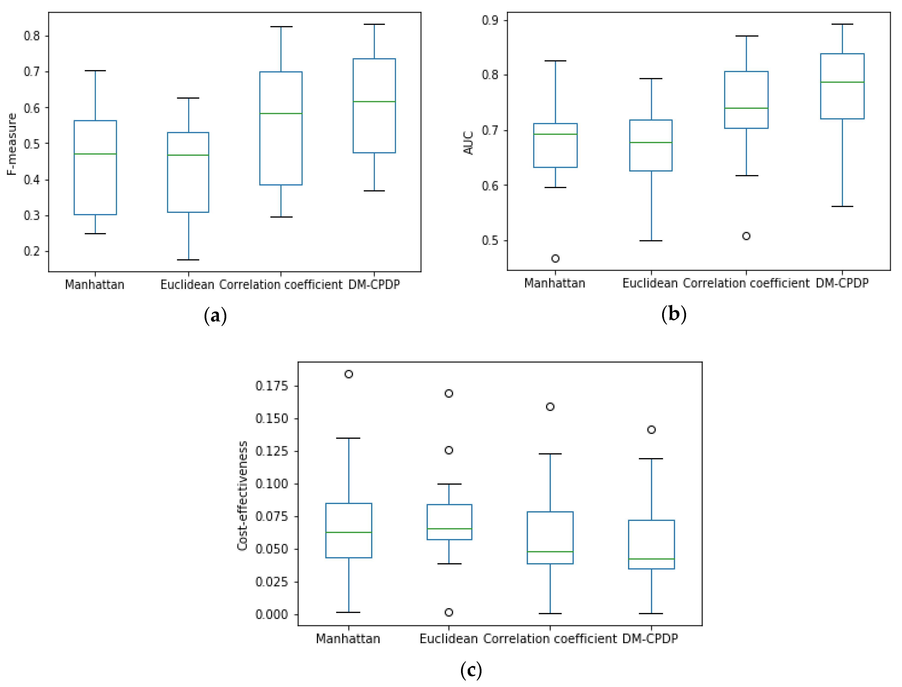
Figure 4 is the box plot of performance indicators, which compare the values of several different dissimilarity metric methods on F-measure, AUC, and cost-effectiveness. Euclidean distance, Manhattan distance, and correlation coefficient are chosen as the measurement of dissimilarity.

The experimental results show that the prediction model using Manhattan distance and Euclidean distance as the measurements of dissimilarity are poor. The value of median, quartile, maximum, and minimum on F-measure and AUC are lower than the arc-cosine kernel. These values on cost-effectiveness are higher than the arc-cosine kernel. During the course of the experiment, we found that the average values of the arc-cosine kernel method on F-measure and AUC are still higher than those three methods, and cost-effectiveness index of arc-cosine kernel method is lower than other methods. In addition, it can be seen from the box plot that when the correlation coefficient is used as the measuring method, the value of median, quartile, maximum, and minimum on F-measure, AUC, and cost-effectiveness are still inferior to the arc-cosine kernel, but superior to the Manhattan and Euclidean distances.

The reasons for these results are as follows. When the relationship between samples is measured by Euclidean distance and Manhattan distance, if the sample and the prototype data are highly correlated, the attribute value of the sample in the dissimilarity space is lower. So that the samples with the same distribution to the target set receive less attention in the process of modeling. Correlation coefficient as the measurement is opposite to the above two methods. This method makes the same distribution samples get higher attention when building the classifier. The arc-cosine kernel function is superior to other methods because the kernel function can better represent the intrinsic relationship between samples, and more attention can be paid to the data that is highly correlated with the target sample in the process of modeling. So it can be concluded that using the arc-cosine kernel function as the measuring method of dissimilarity between samples works better.

4.3.4. Different Prototype Set Selection Methods

In this part, we compare the effects of several different prototype set selection methods on the experimental results.

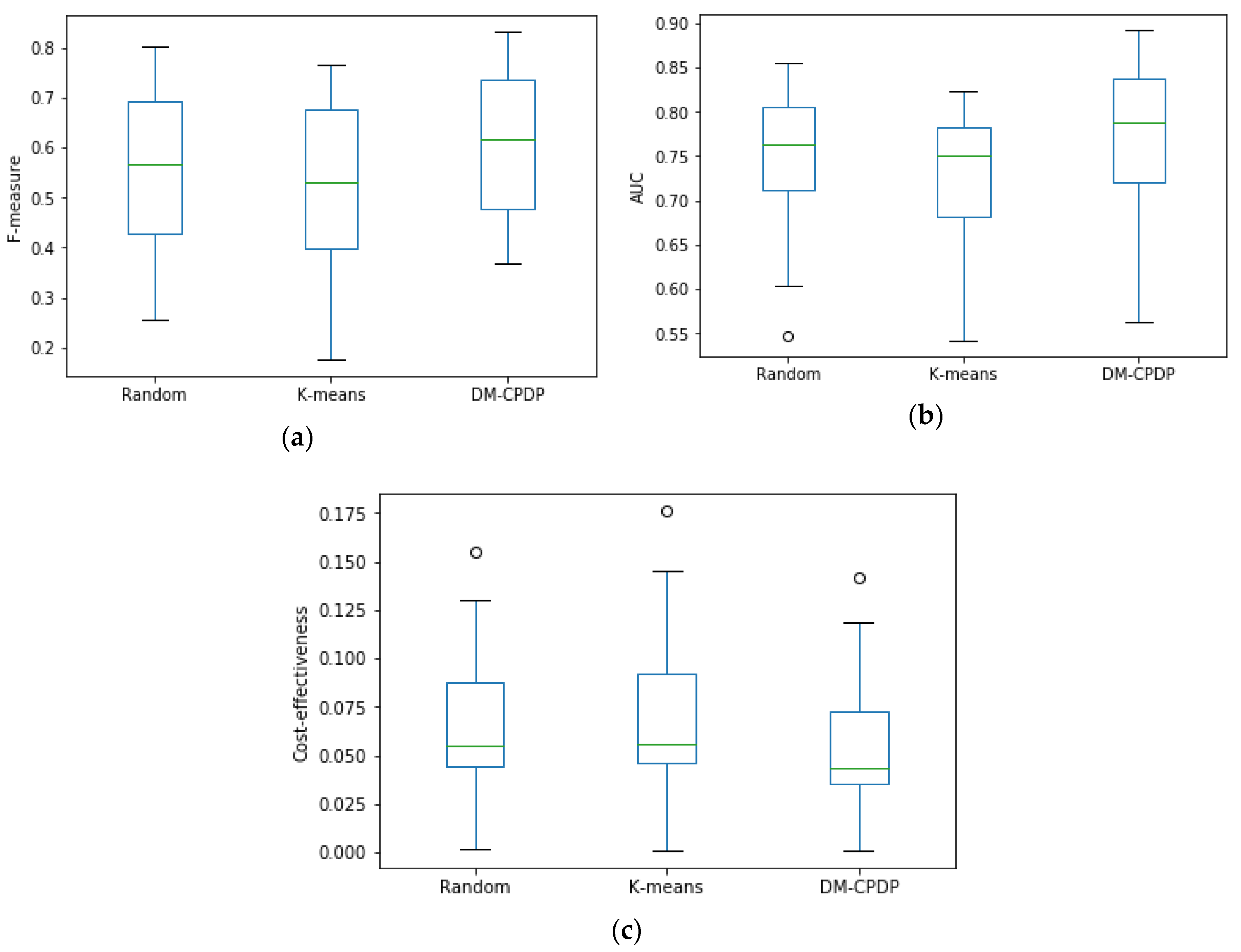
Figure 5 compares three different methods of prototype set selection, namely random algorithm, the K-means algorithm, and the DPC method for DM-CPDP. For the random method, researchers generally select 3%–10% of the dataset [27]. When using the random method to select the prototype set, we select r samples as the prototype set, $r=\log I$ (I is the number of the instance), and repeat the results 10 times to take the mean. When using the K-means method, we also select r samples as the initial cluster center for clustering and select the output cluster center as the prototype set.

It can be seen from the box plot that the density-based prototype selection method used in this paper is better than the random selection method and the K-means clustering method. In Figure 5, the density-based prototype selection method used by the DM-CPDP has higher value of median, quartile, maximum, and minimum on the F-measure and AUC than the other two methods. These cost-effectiveness values for density-based prototype selection method are lower than other methods. However, the K-means clustering method performs the worst, so this method is not suitable for prototype selection.

The reason for this problem is that the K-means algorithm is not suitable for solving non-spherical clusters and is greatly affected by outliers. Although the average effect of random selection is ideal, the prediction results are unstable due to the randomness of the instance selection. Therefore, it is reasonable to use the DPC method for prototype selection.

4.3.5. Experiment on Different Dataset Selection Methods

In this part of the experiment, we compare the effects of different dataset selection methods on the experimental results, bold numbers indicate optimal results on a dataset.

Since the samples have been mapped into the dissimilarity space, the dataset selection method based on extracting the feature vectors is no longer applicable. Thus, we compare the EMD with another method. In each dissimilarity subspace, we select the value of the smallest attribute in each sample and take the mean value to measure the similarity between the source domain data set and the prototype set. Then, the values are sorted in descending order and the first α datasets are selected as the training data. This approach is named as Method 1 [7]. The calculation is as follows:

$$D_{XR}=\frac{1}{n}{\displaystyle \sum }_{i=1}^n\underset{r}{min}k\left(x_i,p_j\right)1\le i\le n,1\le j\le r$$

(17)

The experimental results are shown in

Table 10. Different dataset selection method.

Data Set		Method1			DM-CPDP
	F-Measure	AUC	Cost-Effectiveness	F-Measure	AUC	Cost-Effectiveness
NASA to NASA
CM1	0.591	0.784	0.047	0.594	0.782	0.039
PC1	0.627	0.799	0.035	0.635	0.810	0.027
PC2	0.229	0.558	0.001	0.368	0.563	0.001
PC3	0.770	0.830	0.028	0.776	0.842	0.022
PC4	0.369	0.724	0.070	0.468	0.735	0.061
PC5	0.648	0.762	0.062	0.647	0.768	0.057
KC1	0.801	0.879	0.054	0.832	0.892	0.047
KC2	0.682	0.837	0.043	0.684	0.853	0.035
KC3	0.346	0.681	0.096	0.450	0.685	0.084
KC4	0.504	0.802	0.139	0.502	0.793	0.142
MC1	0.768	0.814	0.037	0.755	0.836	0.039
MC2	0.582	0.645	0.132	0.597	0.662	0.119
MW1	0.371	0.715	0.085	0.393	0.715	0.076
JM1	0.788	0.827	0.044	0.811	0.839	0.036
average	0.577	0.761	0.062	0.608	0.770	0.056
NASA to SOFTLAB
ar3	0.765	0.779	0.043	0.781	0.790	0.040
ar4	0.724	0.782	0.051	0.753	0.837	0.042
ar5	0.848	0.869	0.033	0.863	0.885	0.031
average	0.779	0.810	0.042	0.799	0.837	0.038

. The results show that the performance of dataset selection method based on EMD is superior to Method1 in F-measure, AUC, and cost-effectiveness. The reason for this phenomenon is that when comparing the similarity between datasets, Method 1 has lost more information by selecting the minimum attribute and averaging these attribute values, which leads to inaccurate measurement results. However, the EMD method takes into account each attribute of the sample, so the performance of the prediction model is better.

5. Threats to Validity

The main factor affecting the internal validity of the experiment is the deviation in the code implementation process. For example, we use the HYDRA algorithm for comparison. The algorithm needs to use the genetic algorithm in the implementation, but the random factors of the genetic algorithm may deviate from the experimental results. In view of this problem, this paper eliminates the randomness of the algorithm through repeated tests in the code implementation process. In addition, we compare the results of the reproduce algorithm with the data in the previous papers, which is basically consistent with the results in the previous papers.

The factors that influence the external validity of the experiment are the quality of the datasets and generalization. In view of the quality problem of dataset, we choose NASA and SOFTLAB from PROMISE, which are publicly available datasets often used by researchers. Each dataset contains different project data to reduce the overall impact of data quality on experimental results. In terms of generalization, the data we used to train the model were derived from two open source data sets. These two open source datasets contain 17 project data for a total of 19458 samples, which guarantee the credibility of the experimental.

The factors affecting the validity of the argument are mainly the selection of performance index and comparison algorithms. For the performance index factor, we use the F-measure, AUC, and cost-effectiveness to measure the performance of the model. F-measure is one of the most commonly used evaluation criteria in defect prediction, which can measure the balance between recall and precision. AUC is an indicator that evaluates the overall performance of the model. Cost-effectiveness is used to evaluate the cost of defect inspection in defect prediction. For the problem of comparison algorithms, we choose three representative algorithms, which are cited by many researchers as comparison algorithms. By comparing with these classic algorithms, we can prove the generality of our algorithm.

6. Conclusions

The contribution of this paper is to put forward the method of establishing the cross-project defect prediction module in the dissimilarity space, which provides a new research idea for CPDP. The basic idea of this paper is to use the density-based clustering method to automatically select the cluster centers from the target set as the prototype set. Then the arc-cosine kernel is used to calculate the dissimilarity between the prototype set and the source domain sample as well as the target sample to form the dissimilarity space. After that the training data set are selected by the EMD method, which calculates the cost of converting the data distribution in the source domain to the same data distribution as the target set, and the corresponding samples with a small cost are selected as the training set in the dissimilarity space. Finally, the prediction model is established by TrAdaBoost algorithm.

In the whole data processing process, we complete two transferring. The first transferring is the dissimilarity measure between samples. In the dissimilarity space, each attribute of each sample is the pairwise dissimilarity between the source domain sample and the prototype sample, and the source domain samples with high correlation to the prototype set have higher measurement values. This method is more flexible than the traditional method of assigning weights to the samples in the feature space. The second transferring is the selection stage of the datasets. In this stage, we make full use of the representation method of samples in the dissimilarity space and use the EMD method to measure the similarity between the source domain dataset and the prototype set. Experiments show that the DM-CPDP method has better prediction performance than the traditional methods.

References

- Zimmermann, T.; Nagappan, N.; Gall, H.; Giger, E.; Murphy, B. Cross-project defect prediction: A large scale experiment on data vs. domain vs. process. In Proceedings of the Symposium on the Foundations of Software Engineering, Amsterdam, The Netherlands, 24–28 August 2009; pp. 91–100. [Google Scholar]
- Chen, X.; Gu, Q.; Liu, W.S.; Liu, S.L.; Ni, C. Research on static software defect prediction method. J. Softw. 2016, 27, 1–25. (In Chinese) [Google Scholar] [CrossRef]
- Catal, C. Software fault prediction: A literature review and current trends. Expert Syst. Appl. 2011, 38, 4626–4636. [Google Scholar] [CrossRef]
- Porto, F.; Minku, L.; Mendes, E.; Simao, A. A systematic study of cross-project defect prediction with meta-learning. IEEE Trans. Softw. Eng. 2018, arXiv:1802.06025, 1–23. [Google Scholar]
- Li, Y.; Huang, Z.Q.; Wang, Y.; Fang, B.W. Cross-project software defect prediction based on multi-source data. J. Jilin Univ. 2016, 46, 2034–2041. (In Chinese) [Google Scholar] [CrossRef]
- Pekalska, E.; Duin, R.P.W. Dissimilarity-based classification for vectorial representations. In Proceedings of the International Conference on Pattern Recognition, Hang Kong, China, 20–24 August 2006; pp. 137–140. [Google Scholar]
- Cheplygina, V.; Tax, D.; Loog, M. Dissimilarity-Based ensembles for multiple instance learning. IEEE Trans. Neural Netw. Learn. Syst. 2016, 27, 1379–1391. [Google Scholar] [CrossRef] [PubMed]
- Ma, Y.; Luo, G.; Zeng, X. Transfer learning for cross-company software defect prediction. Inf. Softw. Technol. 2012, 54, 248–256. [Google Scholar] [CrossRef]
- Dai, W.; Yang, Q.; Xue, G.R.; Yu, Y. Boosting for transfer learning. In Proceedings of the International Conference on Machine Learning, Corvalis, OR, USA, 20–24 June 2007; pp. 193–200. [Google Scholar]
- Yu, X.; Liu, J.; Fu, M.; Ma, C.; Nie, G. A multi-source TrAdaBoost approach for cross-company defect prediction. In Proceedings of the International Conference on Software Engineering & Knowledge Engineering, San Francisco Bay, CA, USA, 1–3 July 2016; pp. 237–242. [Google Scholar]
- Xia, X.; Lo, D.; Pan, S.J.; Nagappan, N. HYDRA: Massively compositional model for cross-project defect prediction. IEEE Trans. Softw. Eng. 2016, 42, 977–998. [Google Scholar] [CrossRef]
- Ren, S.; Zhang, Z.; Liu, Y.; Xie, R. Genetic Algorithm-based Transfer Learning for Cross-Company Software Defect Prediction. J. Syst. Softw. 2017, 10, 45–56. [Google Scholar] [CrossRef]
- Yao, Y.; Doretto, G. Boosting for transfer learning with multiple sources. In Proceedings of the 2010 IEEE Computer Society Conference on Computer Vision and Pattern Recognition, San Francisco, CA, USA, 13–18 June 2010; pp. 1855–1862. [Google Scholar]
- Pekalska, E.; Duin, R.P.W.; Wang, G. Dissimilarity representations allow for building good classifiers. Pattern Recognit. Lett. 2002, 23, 943–956. [Google Scholar] [CrossRef] [Green Version]
- Zhang, X.; Song, Q.; Wang, G. A dissimilarity-based imbalanced data classification algorithm. Appl. Intell. 2015, 42, 544–565. [Google Scholar] [CrossRef]
- Kamei, Y.; Fukushima, T.; Mcintosh, S.; Yamashita, K.; Ubayashi, N.; Hassan, A.E. Studying just-in-time defect prediction using cross-project models. Emp. Softw. Eng. 2016, 21, 2072–2106. [Google Scholar] [CrossRef]
- Fukushima, T.; Kamei, Y.; Mcintosh, S.; Yamashita, K.; Ubayashi, N. An empirical study of just-in-time defect prediction using cross-project models. In Proceedings of the Working Conference on Mining Software Repositories, Hyderabad, India, 31 May–1 June 2014; pp. 172–181. [Google Scholar]
- He, J.Y.; Meng, S.P.; Chen, X.; Wang, Z.; Fan, X.Y. A semi-supervised integration cross-project software defect prediction method. J. Softw. 2017, 28, 1455–1473. (In Chinese) [Google Scholar] [CrossRef]
- Lauge, S.; Loog, M.; Tax, D.M.J.; Lee, W.J.; de Bruijne, M.; Duin, R.P.W. Dissimilarity-Based Multiple Instance Learning. In Proceedings of the Structural, Syntactic, and Statistical Pattern Recognition, Izmir, Turkey, 18–20 August 2010; pp. 129–138. [Google Scholar]
- Shang, Z.; Zhang, L. Software Defect Prediction Using Dissimilarity Measures. In Proceedings of the Pattern Recognition, Chongqing, China, 1–5 September 2010. (In Chinese). [Google Scholar]
- Rodriguez, A.; Laio, A. Clustering by fast search and find of density peaks. Science 2014, 344, 1492–1496. [Google Scholar] [CrossRef] [PubMed] [Green Version]
- Cho, Y. Kernel methods for deep learning. Adv. Neural Inf. Process. Syst. 2009, 28, 342–350. [Google Scholar] [CrossRef]
- Liu, W.; Chen, X.; Gu, Q. Feature selection method based on cluster analysis in software defect prediction. Chin. Sci. Inf. Sci. 2016, 46, 1298–1320. (In Chinese) [Google Scholar] [CrossRef]
- Tax, D.M.J.; Loog, M.; Duin, R.P.W.; Cheplygina, V.; Lee, W.J. Bag dissimilarities for multiple instance learning. In Proceedings of the International Workshop on Similarity-Based Pattern Recognition, Venice, Italy, 28–30 September 2011; pp. 222–234. [Google Scholar]
- Arisholm, E.; Briand, L.C. Data Mining Techniques for Building Fault-proneness Models in Telecom Java Software. In Proceedings of the IEEE Computer Society, Washington, DC, USA, 5–9 November 2007; pp. 215–224. [Google Scholar]
- Zhang, H.; Cheung, S.C. A cost-effectiveness criterion for applying software defect prediction models. In Proceedings of the Joint Meeting on Foundations of Software Engineering, Saint Petersburg, Russian Federation, 18–26 August 2013; pp. 643–646. [Google Scholar]
- Pekalska, E.; Duin, R.; Paclik, P. Prototype selection for dissimilarity-based classifiers. Pattern Recognit. 2006, 39, 189–208. [Google Scholar] [CrossRef] [Green Version]
Figure 1.
The framework of the multi-source cross-project defect prediction method based on dissimilarity space (DM-CPDP).
Figure 2.
Cluster center selection diagram. (a) is the descending arrangement diagram of ; (b) is the display of the cluster center point selected by the graph (a) in the data sample.
Figure 3.
The process of data mapping.
Figure 4.
Box plot of different dissimilarity metric methods. (a) is the situation of each method on F-measure; (b) is the situation of each method on AUC; (c) is the situation of each method on cost-effectiveness. Box plots represent maximum, upper quartile, median, lower quartile and minimum values from top to bottom. In addition, circles represent outliers.
Figure 5.
Box plot of different prototype selection methods. (a) is the situation of each method on F-measure; (b) is the situation of each method on AUC; (c) is the situation of each method on cost-effectiveness. Box plots represent maximum, upper quartile, median, lower quartile, and minimum values from top to bottom. In addition, circles represent outliers.