Tensor Completion Based on Triple Tubal Nuclear Norm


1
School of Physics and Electronic Electrical Engineering, Huaiyin Normal University, Huaian 223300, China
2
School of Electronic and Optical Engineering, Nanjing University of Science and Technology, Nanjing 210094, China
3
Jiangsu Province Key Construction Laboratory of Modern Measurement Technology and Intelligent System, Huaian 223300, China
4
School of Computer Science and Engineering, Nanjing University of Science and Technology, Nanjing 210094, China
5
Jiangsu Yaoshi Software Technology Co., Ltd., Nanjing 211103, China
6
Jiangsu Shuoshi Welding Technology Co., Ltd., Nanjing 211103, China
*
Author to whom correspondence should be addressed.
Algorithms 2018, 11(7), 94; https://doi.org/10.3390/a11070094
Submission received: 21 May 2018
/
Revised: 16 June 2018
/
Accepted: 19 June 2018
/
Published: 28 June 2018
Abstract
:Many tasks in computer vision suffer from missing values in tensor data, i.e., multi-way data array. The recently proposed tensor tubal nuclear norm (TNN) has shown superiority in imputing missing values in 3D visual data, like color images and videos. However, by interpreting in a circulant way, TNN only exploits tube (often carrying temporal/channel information) redundancy in a circulant way while preserving the row and column (often carrying spatial information) relationship. In this paper, a new tensor norm named the triple tubal nuclear norm (TriTNN) is proposed to simultaneously exploit tube, row and column redundancy in a circulant way by using a weighted sum of three TNNs. Thus, more spatial-temporal information can be mined. Further, a TriTNN-based tensor completion model with an ADMM solver is developed. Experiments on color images, videos and LiDAR datasets show the superiority of the proposed TriTNN against state-of-the-art nuclear norm-based tensor norms.
1. Introduction
In recent decades, the rapid progress in multi-linear algebra [1] has provided a firm theoretical foundation for many applications in computer vision [2], data mining [3], machine learning [4], signal processing [5], and many other areas. Benefiting from its multi-way nature, the tensor has power against the vector and matrix in exploiting multi-way information in multi-modal data, like color images [6], videos [7], hyper-spectral images [8], functional magnetic resonance imaging [9], traffic volume data [10], etc. In many computer vision tasks, the data, like color images or videos, may be moderately redundant, then it can be interpreted by fewer latent factors [11]. The low-rank tensor provides a suitable model for such data [12]. The two most well-known low-rank tensor models are the low-CP-rank model [13], which tries to interpret a tensor in the fewest rank-one tensors [14], and the low-Tucker-rank model [15], which seeks a tensor proxy that is simultaneously low-rank along each mode.
In many computer vision applications, like image or video inpainting, one has to tackle the missing values in the observed data tensor due to many circumstances [2,16], including failure of sensors, errors or loss in communication, occlusions or noise in the environment, etc. However, it is obviously unable to fill in the missing entries perfectly since they can take arbitrary values without other priors taken into consideration. The most adopted prior is the low-rank prior assuming the underlying data tensor has low rank. Low-rank tensor completion [2,17] seeks a low-rank tensor to fit the underlying data tensor. It has been a hot research topic due its wide use [18]. In low-rank tensor recovery, the rank minimization problem (RMP) is often formulated [2]. However, the general rank minimization problem and most tensor problems are NP-hard [19,20]. To obtain polynomial-time algorithms, many different tensor rank surrogates have been proposed [2,7,17,21,22,23,24] to substitute the rank functions in RMP. Surrogates of the tensor CP rank and Tucker rank have been broadly studied [7,17,23,25,26,27,28,29].
Recently, a novel low-rank tensor model called the low-tubal-rank model was proposed [22,30]. The core of it is to model the 3D data as a tensor that has low tubal-rank [31], which is defined through a new tensor singular value decomposition (t-SVD) [1,32]. It has been successfully used in modeling multi-way real-world data, such as color images [6], videos [33], seismic data [34], WiFi fingerprint [35], MRI imaging [22], traffic volume data [36], etc. As pointed out in [37], compared with other tensor models, the low-tubal-rank tensor model is superior in capturing a “spatial-shifting” correlation, which is ubiquitous in real-world data arrays.
This paper focuses on low-tubal-rank models for tensor completion. The recently-proposed tensor tubal nuclear norm (TNN) [30] based on t-SVD has shown superiority in imputing missing values in 3D visual data, like color images and videos. Its power lies in exploiting tube (often carrying temporal/channel information) redundancy in a circulant way while preserving the row and column (often carrying spatial information) relationship. A simple and successful variant of TNN, dubbed the twist tubal nuclear norm (t-TNN) [16], instead exploits row redundancy in a circulant way while keeping the tube relationship. However, both of them only exploit one kind of redundancy in a circulant way. In this paper, a new tensor norm dubbed the tensor triple tubal nuclear norm (TriTNN) is proposed to simultaneously exploit the row, column and tube redundancy while preserving the relative tube, row and column relationship. Based on the proposed TriTNN, a tensor completion model is studied and optimized by alternating direction multiplier methods (ADMM) [38]. Experimental results on color images, videos and LiDAR datasets demonstrate that the proposed TriTNN has better performances than other state-of-the-art nuclear norm-based tensor norms.
The paper is organized as follows. Some notations and preliminaries are presented in Section 2. The TriTNN is proposed following the introductions of the most related works in Section 3. The problem formulation and the proposed ADMM algorithm are shown in Section 4. Experimental results are reported in Section 5. We conclude this work in Section 6.
2. Notations and Preliminaries
In this section, the notations and the basic definitions are introduced.
2.1. Notations
Vectors are denoted by bold lower case letters, e.g., , matrices are denoted by bold upper case letters, e.g., , and tensors are denoted by calligraphy letters, e.g., . Given a third-order tensor, its fiber is defined as a 1D vector obtained by fixing all indices, but one, and its slice is a 2D matrix defined by fixing all but two indices. Given a 3D tensor , denotes the entry with index ; denotes the k-th frontal slice. denotes the tensor after performing the fast Fourier transformation along the tube fibers of . Notations and are used to represent the discrete Fourier transformation (DFT) and inverse discrete Fourier transformation (IDFT) along the tube fibers of 3D tensors.
Given a matrix , its nuclear norm is defined as where and are the singular values of in non-ascending order. The inner product between two 3D tensors is defined as The Frobenius norm of a tensor is defined as . The -norm of a tensor is defined as .
2.2. Tensor Singular Value Decomposition
Firstly, five block-based operators, i.e., bvec, bvfold, bdiag, bdfoldand bcirc [1], are introduced. Given a tensor , the block vectorizing and its opposite operation are defined as follows:
the block diag matrix and its opposite operation:
and the block circulant matrix as follows:
Based on the five operators defined above, we are able to give the definition of the tensor t-product.
Definition 1
Viewing a 3D tensor as an matrix of tubes, the tensor t-product is analogous to the matrix multiplication by replacing scalar multiplication with the vector circular convolution between the tubes, as follows:
where • denotes the circular convolution [1] between two tube vector defined as:
Due to the relationship between the circular convolution and the DFT, the t-product in the original domain is equivalent to matrix multiplication of the frontal slices in the Fourier domain [1], i.e.,
The tensor transpose, identity tensor, f-diagonal tensor and orthogonal tensor are further defined.
Definition 2
(Tensor transpose [1]). Let be a tensor of size ; then is the tensor obtained by transposing each of the frontal slices and then reversing the order of transposed frontal Slices 2 through .
Definition 3
(Identity tensor [1]). The identity tensor is a tensor whose first frontal slice is the identity matrix, and all other frontal slices are zero.A
Definition 4
(F-diagonal tensor [1]). A tensor is called f-diagonal if each frontal slice of the tensor is a diagonal matrix.
Definition 5
Based on the concepts defined above, the tensor singular value decomposition (t-SVD) and the tensor tubal rank are established as follows.
Definition 6
(Tensor singular value decomposition and tensor tubal-rank [31]). Any tensor can be decomposed as:
where and are orthogonal tensors and is a rectangular f-diagonal tensor of size .
The tensor tubal rank of is defined to be the number of non-zero tubes of in Equation (4), i.e.,
where is an indicator function whose value is one if the input condition is satisfied, and zero otherwise.
3. The Triple Tubal Nuclear Norm
In this section, we will define the triple tensor tubal nuclear norm, before which the most related norms, i.e., tubal nuclear norm and twist tubal nuclear norm, are introduced first.
3.1. Tubal Nuclear Norm
Based on the preliminaries introduced in Section 2, the tubal nuclear norm is defined as follows:
Definition 7
(Tubal nuclear norm [31]). The tubal nuclear norm (TNN) of a 3D tensor is defined as the nuclear norm of the block diagonal matrix of (the Fourier domain version of ), i.e.,
From Definition 7, we can compute the TNN of a tensor efficiently through first conducting FFT along the tube direction and summing the nuclear norms of each frontal slice. Given a tensor , the computation cost of is . Since a block circulant matrix can be block diagonalized through the Fourier transform [1], we obtain:
where ⊗ denotes the Kronecker product [14], is the discrete Fourier transform matrix and is an identity matrix. Note that is a unitary matrix.
The tubal nuclear norm has been used as a convex relaxation of the tensor tubal-rank for tensor completion, tensor robust principle component analysis (TRPCA) and outlier robust tensor principle component analysis (OR-TPCA) [6,30,36,39]. In optimization over TNN, one often needs to compute the proximal operator [40] of TNN defined as:
In [3], a closed-form expression of is given as follows:
Definition 8
([3]). For a 3D tensor with reduced t-SVD , where and are orthogonal tensors and is the f-diagonal tensor of singular tubes, the proximal operator at can be computed through the following equation:
3.2. Twist Tubal Nuclear Norm
The twist tubal nuclear norm [16] is related to a pair of tensor operations named column twist and column squeeze as follows.
Definition 9
(Tensor column twist and column squeeze (here, the twist and squeeze operations in [1,16] are renamed as column twist and column squeeze, respectively, since we will define the row twist and row squeeze) [16]). Let , then the column twist tensor is a tensor of size whose lateral slice . Correspondingly, the column squeeze tensor of , i.e., , can be obtained by the reverse process, i.e., . See Figure 2.
Then, we give the definition of twist nuclear norm as follows:
Definition 10
(Twist tensor nuclear norm [16]). The twist tensor nuclear norm (t-TNN) based on the t-SVD framework is defined as follows:
From the above definition, t-TNN can be computed efficiently by first twisting the original tensor and then computing the TNN. Given a tensor , the computation cost of is . The t-TNN has attained significant improvement against the TNN in video inpainting [16]. Since the t-TNN is essentially a TNN, the proximal operator of it can be derived from the proximal operator of TNN as follows:
3.3. A Circular Interpretation of TNN and t-TNN
In this subsection, an illustration of TNN and t-TNN in a circular way [16], which motivates the proposal of TriTNN, will be given. For a tensor , we define the operation called circulant block matricization of [41] in the following equation:
where denotes an matrix with in the following way:
By the permutation operation, there exist two so-called stride permutation matrices [42] and , such that the following relationship between circ() and bcirc() holds:
Since the matrix nuclear norm is permutation invariant, it holds that [16]:
As an example, Figure 3a,b intuitively shows the relationships between the original tensor, the column twist tensor, the block circulant matrix and the circulant block matricization of a tensor . As illustrated in Subplots (a) and (b) of Figure 3, from the circulant perspective, TNN essentially exploits the tube redundancy in a circulant way while keeping the row and column relationship, and t-TNN essentially exploits the row redundancy in a circulant way while preserving the tube and column relationship [16]. In computer vision applications, the row and column of a data tensor (like color images or videos) often carry spatial information, and the tube often carries temporal or channel information. From the computational perspective, FFT is operated along the tube direction to compute TNN, while t-TNN needs FFT along the row direction.
3.4. The Proposed Row Twist Tubal Nuclear Norm and Triple Tubal Nuclear Norm
As discussed above, TNN and t-TNN need FFT along the tube and row direction, respectively. Note that, for real-word visual data, like color images, the row and column carry homogeneous information, and they are better treated equally. A simple operation similar to the column twist and column squeeze, called row twist and row squeeze, respectively, is defined.
Definition 11
(Tensor row twist and row squeeze). Let , then the row twist tensor is a tensor of size whose horizontal slice . Correspondingly, the row squeeze tensor of , i.e., , can be obtained by the reverse process, i.e., . See Figure 4.
Definition 12
(Row twist tubal nuclear norm (rt-TNN)). The row twist tubal nuclear norm (rt-TNN) of a tensor is defined as the tubal nuclear norm of its row twisted tensor, i.e.,
As illustrated in Subplot (c) of Figure 3, from the circulant perspective, rt-TNN essentially exploits the column redundancy in a circulant way while keeping the row and tube relationship. From the computational perspective, FFT is operated along the column direction to compute rt-TNN. The proximal operator of rt-TNN can be derived from the proximal operator of TNN as follows:
It should be noted that each of TNN, t-TNN and rt-TNN only exploits one type of redundancy, i.e., the tube, row and column redundancies, in a circulant way. Real-world data may have more than one type of redundancy, and it is beneficial to exploit such a property. To simultaneously exploit the tube, row and column redundancy in a circulant way while keeping other relationships, we simply combine the TNN, t-TNN and rt-TNN to get the triple tubal nuclear norm.
Definition 13
(Triple tubal nuclear norm). The triple tubal nuclear norm (TriTNN) is defined as a weighted sum of its tubal nuclear norm, column twist tubal nuclear norm and its row twist tubal nuclear norm, i.e.,
where and are positive weights satisfying:
From the above definition, the computation of can be divided into computations of TNN, t-TNN and rt-TNN, which has the following computational complexity:
Due to the coupling of three tubal nuclear norms, it is very difficult to derive a closed-form expression of the proximal operator of TriTNN.
4. TriTNN-Based Tensor Completion
4.1. Problem Formulation
Let be the true, but unknown tensor to be completed. Suppose only a small fraction of its entries are observed and the observations are corrupted by small dense noise. Let denote the observed noisy tensor of . Then, we have the following observation model:
where is the noise tensor with element-wisely i.i.d. Gaussian noise, ⊙ denotes the element-wise multiplication and denotes the binary tensor whose entry if the -th entry is observed, otherwise . The goal is to estimate given noisy observation from observation Model (19).
We estimate by simultaneously exploiting the tube, row and column redundancy in a circular way through minimizing the proposed triple tubal nuclear norm. Specifically, we come up with the following problem:
where parameter denotes the noise level. The motivation is to recover by choosing the tensor with the smallest TriTNN from a hyper-ball in with radius . It is well known that Problem (20) in the form of convex minimization with a bounded norm constraint is equivalent to the following unconstrained problem [23]:
where is the regularization parameter.
4.2. An ADMM Solver to Problem (21)
The alternative direction multiplier method (ADMM) [38] has been extensively used in solving composite convex problems like Problem (21). We will solve Problem (21) by using ADMM in this subsection.
Considering the definition of TriTNN, we introduce auxiliary variables and obtain the following constrained problem:
First, the augmented Lagrangian of Problem (22) is:
where and are Lagrangian multipliers and is the penalty parameter.
Using the framework of ADMM, we update the variables alternatively by fixing others at the -th iteration in the following way.
Update . We update by fixing the other variables as follows:
where ⊘ denotes element-wise division and denotes the tensor of all ones.
Update , and . Tensor is updated as follows:
where is the proximal operator of TNN at point with parameter (see Equation (8)).
Tensors and are updated similarly to ,
and:
Update and . Using dual ascending, we update and as follows:
We summarize the algorithm in Algorithm 1 and analyze the computational complexity as follows.
Complexity analysis: The main computational cost in each iteration rests in the singular tube thresholding operator, requiring the computation of FFT, IFFT and SVDs. Therefore, the time complexity in each iteration is:
| Algorithm 1 Solving Problem (21) using ADMM. |
| Input: The observed tensor , the parameters . |
| Output:. |
4.3. Convergence of Algorithm 1
As Problem (21) has more than two variables, the convergence property of Algorithm 1 cannot be directly obtained from existing results on the convergence of ADMM [38]. Thus, we prove its convergence in terms of the objective function in the following theorem.
Theorem 1
(Convergence of Algorithm 1). For any , if the unaugmented Lagrangian has a saddle point, then the iterations in Algorithm 1 satisfy the residual convergence, objective convergence and dual variable convergence of Problem (21).
Proof.
The key idea of the proof is to rewrite Problem (9) into a two-block ADMM problem. Since the RowTwist and ColTwist operations are linear, there exist two matrices , such that the constraints and are equivalent to the vectorization expressions:
where denotes the operation of tensor vectorization (see [14]).
For notational simplicity, let:
and:
It is obvious that and are closed, proper and convex. Then, Problem (21) can be re-written as follows:
According to the convergence analysis in [38], we have:
where are the optimal values of , , respectively. Variable is a dual optimal point defined as:
where is the dual component of a saddle point of the unaugmented Lagrangian . □
4.4. Differences from Prior Work
First, we show the difference between the proposed model TriTNN and two mostly related models TNN [30] and t-TNN [16]. Although all of them are based on the tubal nuclear norm, the main difference lies in that TNN and t-TNN only use information of one orientation, whereas TriTNN uses information of three orientations.
Now, we compare the proposed model with Tubal-Alt-Min [37]. It is based on tensor tubal rank and employs the tensor factorization strategy for tensor completion. The differences between TriTNN and Tubal-Alt-Min are: (a) TriTNN preserves the low-rank structure by summing three tubal nuclear norms, whereas Tubal-Alt-Min adopts low-rank tensor factorization to characterize the low-rank property of a tensor. In this way, they are two different kinds of models for tensor completion (since Tubal-Alt-Min and the proposed TriTNN are quite different algorithms and the main goal of this paper is to improve upon TNN, we do not compare Tubal-Alt-Min in the experiment section.) (b) Since TriTNN is based on the tubal nuclear norm, it is formulated as a convex optimization problem (21). Benefiting from convexity, each local minimum of Problem (21) must be a global minimum. However, Tubal-Alt-Min is formulated as a non-convex optimization problem, thus it may produce sub-optimal solutions.
5. Experiments
In this section, extensive experiments will be conducted to explore the effectiveness of the proposed Algorithm 1. All the codes are implemented in MATLAB language, and all experiments are carried out in Windows 10 based on an Intel Core(TM) 2.60-GHz CPU with 12 G RAM.
To explore the effectiveness of the proposed TriTNN-based model, we compare with the following nuclear norm-based tensor completion models:
- The tensor nuclear norm-based model with ADMM solver: high accuracy low-rank tensor completion (HaLRTC, denoted by SNNin this paper) (code available: http://www.cs.rochester.edu/u/jliu/publications.html) [2], The tensor nuclear norm is defined as the weighted sum of nuclear norms of the unfolding matrices along each mode (thus, we denote this model as SNN):where , are positive parameters and , , is the unfolding matrix of tensor along the i-th mode [2].
- The latent tensor nuclear norm-based model (LatentNN) (code available: https://github.com/ryotat/tensor) [21]. The latent tensor nuclear norm is defined as:where and are the first-mode, second-mode and third-mode unfoldings of latent tensors and , respectively.
- The square nuclear norm-based model (SquareNN) (code available: https://sites.google.com/site/mucun1988/publi) [23]. The square nuclear norm of a tensor is defined as the nuclear norm of the most balanced unfolding of a tensor (see [7,23]).
- The most related tubal nuclear norm-based model (TNN) (code available: https://github.com/jamiezeminzhang/) [30] and the twist tubal nuclear norm-based model (t-TNN) [16].
We conduct tensor completion experiments on color images, videos and a dataset for autonomous vehicle. For an estimation tensor , its quality is evaluated by the peak signal-to-noise ratio (PSNR) computed by the definition:
where is the underlying tensor. The higher the PSNR value is, the better the recovery performance will be.
5.1. Color Image Inpainting
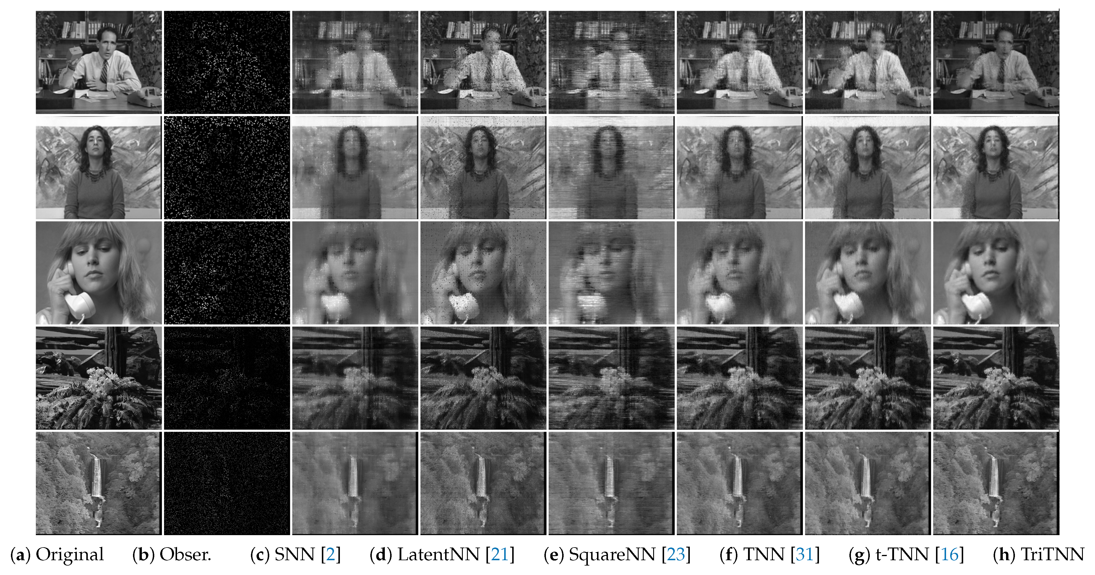
Color images in row × column × channel are naturally expressed in 3D tensor form. Image inpainting aims at reconstructing a color image from a small fraction of its entries. In this experiment, twelve test images of size are used; see Figure 5. Given an image of size , we randomly sample of its pixels and add i.i.d. Gaussian noise with standard deviation , where is the rescaled magnitude of .
The weight parameters of SNN are chosen to satisfy as suggested in [2]. Parameter and in Problem (22) are chosen to satisfy . Parameters of other algorithms are tuned for better performances in most cases. We also employ the structural similarity index measure (SSIM) [43] to measure the quality of inpainted color images. The higher the SSIM value is, the better the inpainting performance will be. Given a color image, we test ten times and report the averaged PSNR and SSIM values.
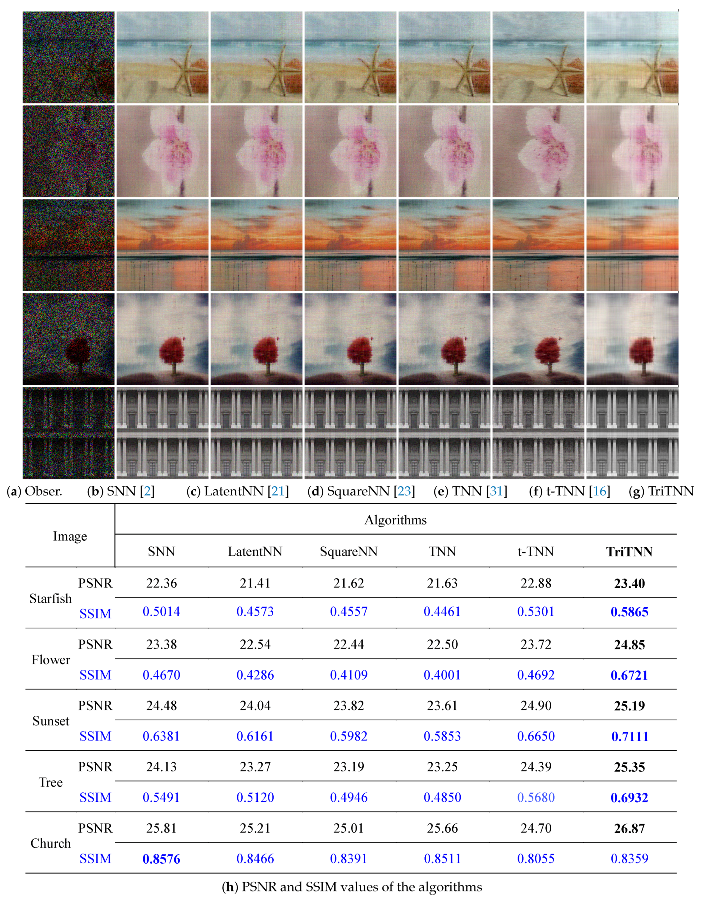
The inpainting results of five images are shown in Figure 6 for qualitative comparison. We can see that the proposed TriTNN-based model obtains better visual performances. For quantitative comparison, the PSNR and SSIM values on the twelve images of seven algorithms are reported in Figure 7. It can be seen that the proposed TriTNN-based outperforms the competitors in most cases.
5.2. Video Inpainting
The video inpainting task aims at imputing the missing pixels of a video. The performance competition is carried out on five widely-used YUVvideos (They are available from https://sites.google.com/site/subudhibadri/fewhelpfuldownloads): salesman_qcif, silent_qcif, suzie_qcif, tempete_cif and waterfall_cif. Due to the computational limitation, we use the first 30 frames of Y components in each video. This results in three tensors sized and two tensors sized . For each video, we uniformly sample 10% of the entries and conduct the video inpainting experiments.
The weight parameters of SNN are chosen to satisfy as suggested in [2]. Parameters -5 and are chosen to satisfy for the proposed model. Parameters of other algorithms are tuned for better performances in most cases. Given a video, we test ten times and report the averaged PSNR value.
The qualitative comparison is shown in Figure 8. The PSNR values are reported in Table 1. It can be seen that the TriTNN-based model outperforms the others. The proposed TriTNN has better performances than TNN and t-TNN, since the TriTNN exploits the row, column and tube redundancy simultaneously, whereas TNN or t-TNN only exploit one type of redundancy. The superiority of TriTNN over SNN, LatentNN and SquareNN may be explained by the fact that the circulant block matricization of a tensor coded in TriTNN makes use of more information than directly unfolding along each mode.
5.3. A Dataset for Autonomous Driving
Environment perception for autonomous driving has attracted more and more attention in computer vision. In this subsection, experiments on a dataset collected for autonomous driving are performed.
The dataset (a collection of Frame No. 165–No. 244 in Scenario B and Scenario B; additional sensor data available at http://www.mrt.kit.edu/z/publ/download/velodynetracking/dataset.html) has 80 frames of gray images and LiDAR point cloud data acquired by a Velodyne HDL-64E LiDAR. The image sequence is resized to be a tensor of size , and the LiDAR data are resampled, transformed and formatted to be two tensors of size representing the distance data and the intensity data, respectively.
Given a tensor to complete , experiments are carried out with seven different observation settings where the sampling ratio p varies from 0.1–0.7. The observed entries are further corrupted by i.i.d. Gaussian noise with standard deviation , where is the normalized magnitude of . The weight parameters of SNN are chosen to satisfy . Parameters -5 and are chosen to satisfy for the proposed model. Parameters of other algorithm are tuned manually to achieve better performances in most cases. Given a sampling ratio p, we repeat ten trials and report the averaged PSNR value.
The quantitative performance comparison in terms of PSNR is shown in Table 2, Table 3 and Table 4 for gray image sequence, distance data and intensity data completion, respectively. The highest average PSNR indicating the best recovery performance is highlighted in bold. From Table 2, Table 3 and Table 4, we can see that the proposed TriTNN-based model yields better performances over the other five algorithms for noisy tensor completion.
6. Conclusions
This paper studied the problem of completing a 3D tensor from incomplete observations. It has been used in broad applications of computer vision tasks like image and video inpainting. In this paper, a new tensor norm named the triple tubal nuclear norm (TriTNN) is proposed to simultaneously exploit tube, row and column redundancy in a circulant way by using a weighted sum of three TNNs. A TriTNN-based tensor completion model is presented. It is further solved by an ADMM-based algorithm with convergence guarantee. Experimental results on color images, videos and LiDAR datasets show the superiority of the proposed TriTNN against state-of-the-art nuclear norm-based tensor norms.
For the proposed TriTNN, the authors believe it can outperform many nuclear norm-based tensor completion models because more spatial-temporal information is exploited. However, generally speaking, it has the following two drawbacks:
- Computational inefficiency: Compared to TNN and t-TNN, it is more time-consuming since it involves computing TNN, t-TNN and rt-TNN (see Equation (18)).
In the future research, the authors are interested in efficient algorithms like [45] to tackle the problem of computational inefficiency. To decrease the sample complexity of TriTNN, it will be helpful to follow the suggestions in [44] to design new atomic norms like [46]. To get better visual completion performances, the authors would like to consider adding smoothness regularization in the model like [47,48,49] and adopting different tensorization methods like [50]. It is also helpful for studying new tensor completion models using deep neural networks [51]. For potential extensions of TriTNN, the authors would like to explore the p-th order () extension [52] and extensions to other discrete transforms other than DFT like [53].
Author Contributions
Conceptualization, D.W. and A.W. Data curation, D.W. and X.F. Formal analysis, B.W. (Bo Wang). Methodology, D.W. and A.W. Resources, B.W. (Boyu Wang) and B.W. (Bo Wang). Software, X.F. and B.W. (Boyu Wang). Writing, original draft, D.W., A.W. and X.F. Writing, review and editing, B.W. (Boyu Wang) and B.W. (Bo Wang).
Acknowledgments
The authors are grateful to the anonymous referees for their insightful and constructive comments that led to an improved version of the paper. The authors would like to thank Fangfang Yang and Zhong Jin for their long-time support. The authors wish to thank the audiences of White Paper Tao (WPT) for their focus.This work is partially supported by the National Natural Science Foundation of China under Grant Nos. 61702262, 61703209, 91420201 and 61472187.
Conflicts of Interest
The authors declare no conflict of interest.
References
- Kilmer, M.E.; Braman, K.; Hao, N.; Hoover, R.C. Third-order tensors as operators on matrices: A theoretical and computational framework with applications in imaging. SIAM J. Matrix Anal. Appl. 2013, 34, 148–172. [Google Scholar] [CrossRef]
- Liu, J.; Musialski, P.; Wonka, P.; Ye, J. Tensor completion for estimating missing values in visual data. IEEE Trans. Pattern Anal. Mach. Intell. 2013, 35, 208–220. [Google Scholar] [CrossRef] [PubMed]
- Wang, A.; Jin, Z. Near-optimal Noisy Low-tubal-rank Tensor Completion via Singular Tube Thresholding. In Proceedings of the IEEE International Conference on Data Mining Workshop (ICDMW), New Orleans, LA, USA, 18–21 November 2017; pp. 553–560. [Google Scholar]
- Signoretto, M.; Dinh, Q.T.; Lathauwer, L.D.; Suykens, J.A.K. Learning with tensors: a framework based on convex optimization and spectral regularization. Mach. Learn. 2014, 94, 303–351. [Google Scholar] [CrossRef]
- Cichocki, A.; Mandic, D.; De Lathauwer, L.; Zhou, G.; Zhao, Q.; Caiafa, C.; Phan, H.A. Tensor decompositions for signal processing applications: From two-way to multiway component analysis. IEEE Signal Process. Mag. 2015, 32, 145–163. [Google Scholar] [CrossRef]
- Lu, C.; Feng, J.; Chen, Y.; Liu, W.; Lin, Z.; Yan, S. Tensor Robust Principal Component Analysis: Exact Recovery of Corrupted Low-Rank Tensors via Convex Optimization. In Proceedings of the IEEE Conference on Computer Vision and Pattern Recognition, Las Vegas, NV, USA, 27–30 June 2016; pp. 5249–5257. [Google Scholar]
- Wei, D.; Wang, A.; Wang, B.; Feng, X. Tensor Completion Using Spectral (k, p) -Support Norm. IEEE Access 2018, 6, 11559–11572. [Google Scholar] [CrossRef]
- Liu, Y.; Shang, F. An Efficient Matrix Factorization Method for Tensor Completion. IEEE Signal Process. Lett. 2013, 20, 307–310. [Google Scholar] [CrossRef]
- Song, X.; Lu, H. Multilinear Regression for Embedded Feature Selection with Application to fMRI Analysis. In Proceedings of the AAAI Conference on Artificial Intelligence, San Francisco, CA, USA, 4–9 February 2017; pp. 2562–2568. [Google Scholar]
- Tan, H.; Feng, G.; Feng, J.; Wang, W.; Zhang, Y.J.; Li, F. A tensor-based method for missing traffic data completion. Transp. Res. Part C 2013, 28, 15–27. [Google Scholar] [CrossRef]
- Zhao, Q.; Zhang, L.; Cichocki, A. Bayesian CP Factorization of Incomplete Tensors with Automatic Rank Determination. IEEE Trans. Pattern Anal. Mach. Intell. 2015, 37, 1751–1763. [Google Scholar] [CrossRef] [PubMed]
- Cichocki, A.; Lee, N.; Oseledets, I.; Phan, A.H.; Zhao, Q.; Mandic, D.P. Tensor Networks for Dimensionality Reduction and Large-scale Optimization: Part 1 Low-Rank Tensor Decompositions. Found. Trends Mach. Learn. 2016, 9, 249–429. [Google Scholar] [CrossRef] [Green Version]
- Harshman, R.A. Foundations of the PARAFAC Procedure: Models and Conditions for an “Explanatory” Multi-Modal Factor Analysis; University of California: Los Angeles, CA, USA, 1970. [Google Scholar]
- Kolda, T.G.; Bader, B.W. Tensor decompositions and applications. SIAM Rev. 2009, 51, 455–500. [Google Scholar] [CrossRef]
- Tucker, L.R. Some mathematical notes on three-mode factor analysis. Psychometrika 1966, 31, 279–311. [Google Scholar] [CrossRef] [PubMed]
- Hu, W.; Tao, D.; Zhang, W. The twist tensor nuclear norm for video completion. IEEE Trans. Neural Netw. Learn. Syst. 2017, 28, 2961–2973. [Google Scholar] [CrossRef] [PubMed]
- Yuan, M.; Zhang, C.H. Incoherent Tensor Norms and Their Applications in Higher Order Tensor Completion. IEEE Trans. Inf. Theory 2017, 63, 6753–6766. [Google Scholar] [CrossRef] [Green Version]
- Song, Q.; Ge, H.; Caverlee, J.; Hu, X. Tensor Completion Algorithms in Big Data Analytics. arXiv, 2017; arXiv:1711.10105. [Google Scholar]
- Candès, E.J.; Tao, T. The power of convex relaxation: near-optimal matrix completion. IEEE Trans. Inf. Theory 2010, 56, 2053–2080. [Google Scholar] [CrossRef]
- Hillar, C.J.; Lim, L. Most Tensor Problems Are NP-Hard. J. ACM 2009, 60, 45. [Google Scholar] [CrossRef]
- Tomioka, R.; Suzuki, T. Convex tensor decomposition via structured schatten norm regularization. In Proceedings of the Advances in Neural Information Processing Systems, Lake Tahoe, NV, USA, 5–10 December 2013; pp. 1331–1339. [Google Scholar]
- Semerci, O.; Hao, N.; Kilmer, M.E.; Miller, E.L. Tensor-Based Formulation and Nuclear Norm Regularization for Multienergy Computed Tomography. IEEE Trans. Image Process. 2014, 23, 1678–1693. [Google Scholar] [CrossRef] [PubMed] [Green Version]
- Mu, C.; Huang, B.; Wright, J.; Goldfarb, D. Square Deal: Lower Bounds and Improved Relaxations for Tensor Recovery. In Proceedings of the International Conference on Machine Learning, Beijing, China, 21–26 June 2014; pp. 73–81. [Google Scholar]
- Zhao, Q.; Meng, D.; Kong, X.; Xie, Q.; Cao, W.; Wang, Y.; Xu, Z. A Novel Sparsity Measure for Tensor Recovery. In Proceedings of the IEEE International Conference on Computer Vision, Santiago, Chile, 7–13 December 2015; pp. 271–279. [Google Scholar]
- Tomioka, R.; Hayashi, K.; Kashima, H. Estimation of low-rank tensors via convex optimization. arXiv, 2010; arXiv:1010.0789. [Google Scholar]
- Chretien, S.; Wei, T. Sensing tensors with Gaussian filters. IEEE Trans. Inf. Theory 2017, 63, 843–852. [Google Scholar] [CrossRef]
- Ghadermarzy, N.; Plan, Y.; Yılmaz, Ö. Near-optimal sample complexity for convex tensor completion. arXiv, 2017; arXiv:1711.04965. [Google Scholar]
- Ghadermarzy, N.; Plan, Y.; Yılmaz, Ö. Learning tensors from partial binary measurements. arXiv, 2018; arXiv:1804.00108. [Google Scholar]
- Liu, Y.; Shang, F.; Fan, W.; Cheng, J.; Cheng, H. Generalized Higher-Order Orthogonal Iteration for Tensor Decomposition and Completion. In Proceedings of the Advances in Neural Information Processing Systems, Palais des Congrès de Montréal, Montréal, Canada, 8–13 December 2014; pp. 1763–1771. [Google Scholar]
- Zhang, Z.; Ely, G.; Aeron, S.; Hao, N.; Kilmer, M. Novel methods for multilinear data completion and de-noising based on tensor-SVD. In Proceedings of the IEEE Conference on Computer Vision and Pattern Recognition, Columbus, OH, USA, 23–28 June 2014; pp. 3842–3849. [Google Scholar]
- Zhang, Z.; Aeron, S. Exact Tensor Completion Using t-SVD. IEEE Trans. Signal Process. 2017, 65, 1511–1526. [Google Scholar] [CrossRef]
- Sun, W.; Chen, Y.; Huang, L.; So, H.C. Tensor Completion via Generalized Tensor Tubal Rank Minimization using General Unfolding. IEEE Signal Process. Lett. 2018. [Google Scholar] [CrossRef]
- Zhou, P.; Lu, C.; Lin, Z.; Zhang, C. Tensor Factorization for Low-Rank Tensor Completion. IEEE Trans. Image Process. 2018, 27, 1152–1163. [Google Scholar] [CrossRef] [PubMed]
- Ely, G.T.; Aeron, S.; Hao, N.; Kilmer, M.E. 5D seismic data completion and denoising using a novel class of tensor decompositions. Geophysics 2015, 80, V83–V95. [Google Scholar] [CrossRef]
- Liu, X.; Aeron, S.; Aggarwal, V.; Wang, X.; Wu, M. Adaptive Sampling of RF Fingerprints for Fine-grained Indoor Localization. IEEE Trans. Mob. Comput. 2016, 15, 2411–2423. [Google Scholar] [CrossRef]
- Jiang, J.Q.; Ng, M.K. Exact Tensor Completion from Sparsely Corrupted Observations via Convex Optimization. arXiv, 2017; arXiv:1708.00601. [Google Scholar]
- Liu, X.Y.; Aeron, S.; Aggarwal, V.; Wang, X. Low-tubal-rank tensor completion using alternating minimization. arXiv, 2016; arXiv:1610.01690. [Google Scholar]
- Boyd, S.; Parikh, N.; Chu, E.; Peleato, B.; Eckstein, J. Distributed optimization and statistical learning via the alternating direction method of multipliers. Found. Trends Mach. Learn. 2011, 3, 1–122. [Google Scholar] [CrossRef]
- Zhou, P.; Feng, J. Outlier-Robust Tensor PCA. In Proceedings of the IEEE Conference on Computer Vision and Pattern Recognition, Honolulu, HI, USA, 21–26 July 2017. [Google Scholar]
- Cai, J.F.; Candès, E.J.; Shen, Z. A singular value thresholding algorithm for matrix completion. SIAM J. Opt. 2010, 20, 1956–1982. [Google Scholar] [CrossRef]
- Gleich, D.F.; Greif, C.; Varah, J.M. The power and Arnoldi methods in an algebra of circulants. Numer. Linear Algebra Appl. 2013, 20, 809–831. [Google Scholar] [CrossRef]
- Granata, J.; Conner, M.; Tolimieri, R. The tensor product: a mathematical programming language for FFTs and other fast DSP operations. IEEE Signal Process. Mag. 1992, 9, 40–48. [Google Scholar] [CrossRef]
- Wang, Z.; Bovik, A.C.; Sheikh, H.R.; Simoncelli, E.P. Image quality assessment: from error visibility to structural similarity. IEEE Trans. Image Process. 2004, 13, 600–612. [Google Scholar] [CrossRef] [PubMed]
- Oymak, S.; Jalali, A.; Fazel, M.; Eldar, Y.C.; Hassibi, B. Simultaneously structured models with application to sparse and low-rank matrices. IEEE Trans. Inf. Theory 2015, 61, 2886–2908. [Google Scholar] [CrossRef]
- Mu, C.; Zhang, Y.; Wright, J.; Goldfarb, D. Scalable Robust Matrix Recovery: Frank-Wolfe Meets Proximal Methods. SIAM J. Sci. Comput. 2016, 38, A3291–A3317. [Google Scholar] [CrossRef]
- Richard, E.; Obozinski, G.R.; Vert, J.P. Tight convex relaxations for sparse matrix factorization. In Proceedings of the Advances in Neural Information Processing Systems, Montreal, QC, Canada, 8–13 December 2014; pp. 3284–3292. [Google Scholar]
- Yokota, T.; Zhao, Q.; Cichocki, A. Smooth PARAFAC Decomposition for Tensor Completion. IEEE Trans. Signal Process. 2016, 64, 5423–5436. [Google Scholar] [CrossRef]
- Chen, Y.L.; Hsu, C.T.; Liao, H.Y.M. Simultaneous Tensor Decomposition and Completion Using Factor Priors. IEEE Trans. Pattern Anal. Mach. Intell. 2014, 36, 577–591. [Google Scholar] [CrossRef] [PubMed]
- Xutao Li, Y.Y.; Xu, X. Low-Rank Tensor Completion with Total Variation for Visual Data Inpainting. In Proceedings of the AAAI Conference on Artificial Intelligence, San Francisco, CA, USA, 4–9 February 2017; pp. 2210–2216. [Google Scholar]
- Yokota, T.; Erem, B.; Guler, S.; Warfield, S.K.; Hontani, H. Missing Slice Recovery for Tensors Using a Low-rank Model in Embedded Space. arXiv, 2018; arXiv:1804.01736. [Google Scholar]
- Fan, J.; Cheng, J. Matrix completion by deep matrix factorization. Neural Netw. 2018, 98, 34–41. [Google Scholar] [CrossRef] [PubMed]
- Martin, C.D.; Shafer, R.; Larue, B. An Order-p Tensor Factorization with Applications in Imaging. SIAM J. Sci. Comput. 2013, 35, A474–A490. [Google Scholar] [CrossRef]
- Liu, X.Y.; Wang, X. Fourth-order tensors with multidimensional discrete transforms. arXiv, 2017; arXiv:1705.01576. [Google Scholar]
Figure 1.
Illustration of tensor (t)-SVD.
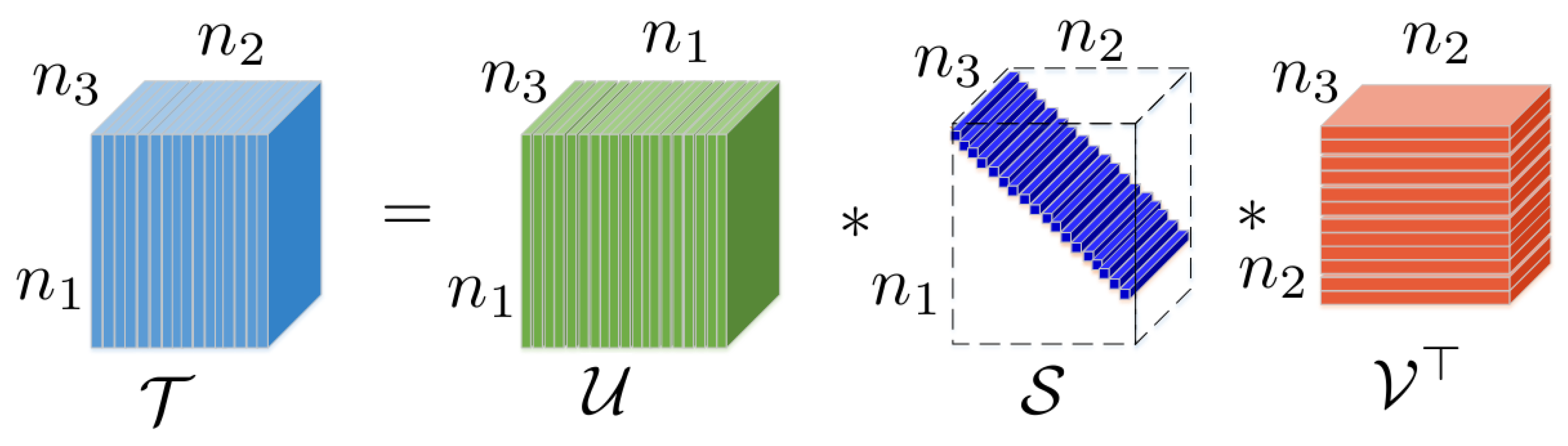
Figure 2.
The column twist and column squeeze operations.
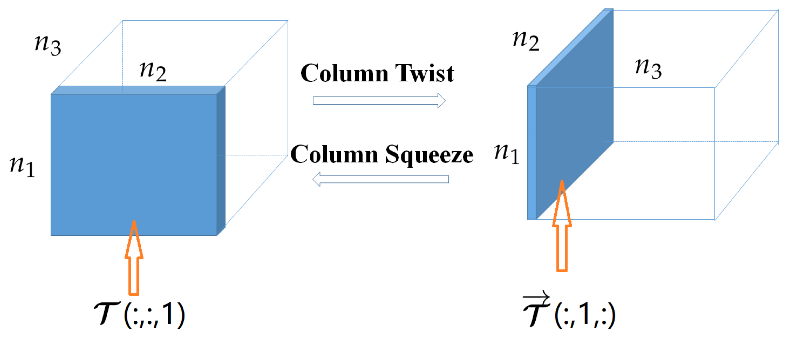
Figure 3.
An intuitive illustration of relationships between the original tensor, the column twist tensor, the row twist tensor, the block circulant matrix and the circulant block matricization of a tensor . Subplots (a–c) show the operations on the column twist tensor, the original tensor and the row twist tensor, respectively. It can be seen that exploits the tube redundancy in a circulant way while keeping the row and column relationship, exploits the row redundancy in a circulant way while keeping the tube and column relationship and exploits the column redundancy in a circulant way while keeping the tube and row relationship.

Figure 4.
The row twist and row squeeze operations.

Figure 5.
Twelve color images used in the experiments.

Figure 6.
Examples of color image inpainting. (a) is the observed noisy incomplete image (Obs.) with sampling ratio 0.3 and noise level ; (b–g) show the inpainting results of nuclear norm-based models: SNN [2], latent tensor nuclear norm-based model (LatentNN) [21], SquareNN [23], tensor tubal nuclear norm (TNN) [31], t-TNN [16] and the proposed model, respectively. The corresponding PSNR and SSIM values are listed in (k). The highest PSNR and SSIM indicating the best inpainting performance are highlighted in bold. It is suggested to be viewed in color as a pdf file with a 4× zoom in. TriTNN, triple tubal nuclear norm.

Figure 7.
Quantitative evaluation of algorithms on color images for Uniform-0.3: the image is sampled uniformly with ratio and corrupted with noise level . (a) PSNR values; (b) SSIM values.
Figure 7.
Quantitative evaluation of algorithms on color images for Uniform-0.3: the image is sampled uniformly with ratio and corrupted with noise level . (a) PSNR values; (b) SSIM values.
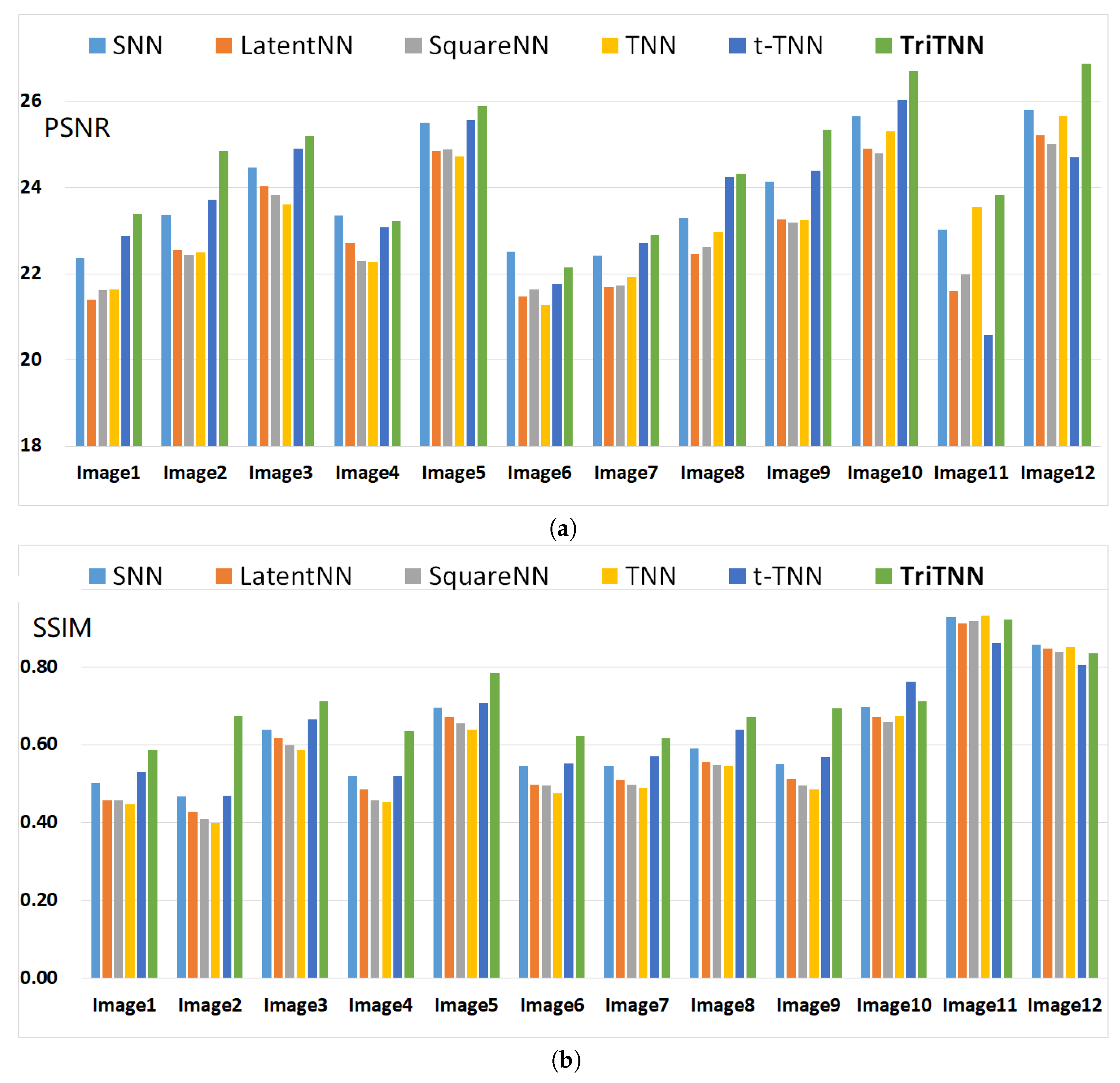
Figure 8.
Examples of YUVvideo inpainting. (a) is the first frame of each video; (b) is the observed incomplete frame (Obs.) with missing entries; (c–h) show the inpainting results of nuclear norm-based models: SNN [2], LatentNN [21], SquareNN [23], TNN [31], t-TNN [16] and the proposed model TriTNN-based model, respectively. It is suggested to be viewed as a pdf file with a 4× zoom in.

Table 1.
Quantitative evaluation of algorithms in PSNR values for YUV video inpainting: each video is sampled uniformly with ratio .
Table 1.
Quantitative evaluation of algorithms in PSNR values for YUV video inpainting: each video is sampled uniformly with ratio .
| Video | SNN [2] | LatentNN [21] | SquareNN [23] | TNN [31] | t-TNN [16] | TriTNN |
|---|---|---|---|---|---|---|
| salesman_qcif | 21.10 | 24.21 | 20.31 | 25.56 | 25.73 | 26.18 |
| silent_qcif | 24.07 | 23.95 | 22.98 | 27.93 | 28.03 | 28.47 |
| suzie_qcif | 25.79 | 24.63 | 24.48 | 27.92 | 29.47 | 29.70 |
| tempete_cif | 19.10 | 18.45 | 19.23 | 20.65 | 21.21 | 21.46 |
| waterfall_cif | 24.10 | 22.39 | 24.06 | 26.71 | 27.44 | 28.22 |
Table 2.
Comparison of the PSNR values for image sequence completion.
| Sampling Ratio | SNN [2] | LatentNN [21] | SquareNN [23] | TNN [31] | t-TNN [16] | TriTNN |
|---|---|---|---|---|---|---|
| 14.58 | 15.50 | 17.27 | 17.23 | 17.29 | 17.45 | |
| 17.79 | 17.27 | 18.16 | 18.32 | 18.59 | 18.74 | |
| 18.74 | 18.36 | 18.80 | 19.04 | 19.12 | 19.53 | |
| 19.29 | 19.02 | 19.21 | 19.50 | 19.44 | 20.02 | |
| 19.61 | 19.43 | 19.49 | 19.82 | 19.64 | 20.28 | |
| 19.80 | 19.70 | 19.69 | 20.06 | 19.76 | 22.01 | |
| 19.90 | 19.83 | 19.84 | 20.23 | 19.85 | 22.41 |
Table 3.
Comparison of the PSNR values for HDL-64Edistance data completion.
| Sampling Ratio | SNN [2] | LatentNN [21] | SquareNN [23] | TNN [31] | t-TNN [16] | TriTNN |
|---|---|---|---|---|---|---|
| 17.80 | 16.90 | 17.64 | 19.03 | 18.67 | 18.91 | |
| 19.26 | 18.48 | 18.94 | 20.04 | 19.60 | 20.09 | |
| 20.33 | 19.71 | 19.94 | 20.93 | 20.41 | 21.04 | |
| 21.24 | 20.67 | 20.89 | 21.74 | 21.17 | 21.92 | |
| 22.05 | 21.55 | 21.75 | 22.47 | 21.88 | 22.72 | |
| 22.82 | 22.39 | 22.56 | 23.16 | 22.61 | 23.68 | |
| 23.54 | 23.21 | 23.34 | 23.79 | 23.35 | 24.51 |
Table 4.
Comparison of the PSNR values for HDL-64E intensity data completion.
| Sampling Ratio | SNN [2] | LatentNN [21] | SquareNN [23] | TNN [31] | t-TNN [16] | TriTNN |
|---|---|---|---|---|---|---|
| 17.30 | 17.63 | 17.57 | 18.31 | 18.62 | 18.36 | |
| 18.79 | 19.30 | 18.92 | 19.50 | 19.61 | 19.63 | |
| 19.85 | 20.29 | 19.93 | 20.38 | 20.37 | 20.45 | |
| 20.84 | 21.11 | 20.90 | 21.24 | 21.08 | 21.30 | |
| 21.72 | 21.86 | 21.76 | 22.05 | 21.78 | 22.18 | |
| 22.51 | 22.62 | 22.53 | 22.79 | 22.50 | 22.94 | |
| 23.39 | 23.40 | 23.39 | 23.59 | 23.27 | 23.80 |
© 2018 by the authors. Licensee MDPI, Basel, Switzerland. This article is an open access article distributed under the terms and conditions of the Creative Commons Attribution (CC BY) license (http://creativecommons.org/licenses/by/4.0/).
Share and Cite
MDPI and ACS Style
Wei, D.; Wang, A.; Feng, X.; Wang, B.; Wang, B. Tensor Completion Based on Triple Tubal Nuclear Norm. Algorithms 2018, 11, 94. https://doi.org/10.3390/a11070094
AMA Style
Wei D, Wang A, Feng X, Wang B, Wang B. Tensor Completion Based on Triple Tubal Nuclear Norm. Algorithms. 2018; 11(7):94. https://doi.org/10.3390/a11070094
Chicago/Turabian StyleWei, Dongxu, Andong Wang, Xiaoqin Feng, Boyu Wang, and Bo Wang. 2018. "Tensor Completion Based on Triple Tubal Nuclear Norm" Algorithms 11, no. 7: 94. https://doi.org/10.3390/a11070094
Note that from the first issue of 2016, this journal uses article numbers instead of page numbers. See further details here.