Control Strategy of Speed Servo Systems Based on Deep Reinforcement Learning


School of Electrical Engineering and Automation, East China Jiaotong University, Nanchang 330013, China
*
Author to whom correspondence should be addressed.
Algorithms 2018, 11(5), 65; https://doi.org/10.3390/a11050065
Submission received: 8 March 2018
/
Revised: 28 April 2018
/
Accepted: 3 May 2018
/
Published: 5 May 2018
(This article belongs to the Special Issue Algorithms for PID Controller)
Abstract
:We developed a novel control strategy of speed servo systems based on deep reinforcement learning. The control parameters of speed servo systems are difficult to regulate for practical applications, and problems of moment disturbance and inertia mutation occur during the operation process. A class of reinforcement learning agents for speed servo systems is designed based on the deep deterministic policy gradient algorithm. The agents are trained by a significant number of system data. After learning completion, they can automatically adjust the control parameters of servo systems and compensate for current online. Consequently, a servo system can always maintain good control performance. Numerous experiments are conducted to verify the proposed control strategy. Results show that the proposed method can achieve proportional–integral–derivative automatic tuning and effectively overcome the effects of inertia mutation and torque disturbance.
1. Introduction
Servo systems are widely used in robots, aerospace, computer numerical control machine tools, and other fields [1,2,3]. Their internal electrical characteristics often change, namely, the inertia change of the mechanical structure connected to them and the torque disturbance in the working process. Servo systems generally adopt a fixed-parameter structure proportional–integral–derivative (PID) controller to complete the system adjustment process. The control performance of the PID controller with a fixed-parameter structure is closely related to its control parameters. When the state of the control loop changes, it will not achieve a good control performance [4,5,6]. Servo systems often need to reorganize their parameters and seek new control strategies to meet the needs of high-performance control in various situations.
Many researchers have proposed several solutions for the problems of inertia variables and torque disturbance in the application of servo systems such as fuzzy logic, synovial, and adaptive control to improve the control accuracy of servo systems. Dong, Vu, and Han et al. [7] proposed a fuzzy neural network adaptive hybrid control system, which obtained high robustness when torque disturbance and servo motor parameters were uncertain. However, a systematic fuzzy control theory was difficult to establish to solve the fuzzy control mechanism. A large number of fuzzy rules also needed to be established to improve control accuracy, which greatly increased the algorithm complexity. Jezernik, Korelič, and Horvat [8] proposed a sliding mode control method for permanent magnet synchronous motors, which can have a fast dynamic response and strong robustness when changes in torque occur. However, when the system parameters were changed, the controller output easily produced jitter. In [9], an adaptive PID control method based on gradient descent method was proposed. The control method presented a fast dynamic response and a small steady-state error when the internal parameters of the servo system changed. However, the algorithm was slow and difficult to converge. Although defects remain in existing PID control methods, the PID control structure is still an important way to improve the control performances of systems.
Deep reinforcement learning is an important branch of artificial intelligence and has made great progress in recent years. In 2015, the Google DeepMind team proposed a deep reinforcement learning algorithm, deep Q-network (DQN) [10,11], and verified its universality and superiority in the games of Atari 2600, StarCraft, and Go [12]. The research progress of deep reinforcement learning has attracted the attention of many researchers. Not only have many improvement strategies been proposed, many researchers have begun to apply the research results of deep reinforcement learning to practical engineering applications. Lillicrap T.P proposed a deep deterministic policy gradient (DDPG) algorithm as a replay buffer to construct a target network to solve the problems of a continuous motion space neural network convergence and a slow algorithm update [13]. Jiang, Zhang, and Luo et al. [14] adopted a reinforcement learning method to realize an optimized tracking control of completely unknown nonlinear Markov jump systems. Carlucho, Paula, and Villar et al. [15] proposed an incremental q-learning adaptive PID control algorithm and applied it to mobile machines. Yu, Shi, and Huang et al. [16] proposed an optimal tracking control of an underwater vehicle based on the DDPG algorithm and achieved better control accuracy than that of the traditional PID algorithm. Other studies such as [17,18] adopted the reinforcement learning of continuous state space to energy management.
The aforementioned results lay a good theoretical foundation, however, there still exist three shortcomings in the control process of a servo system: (1) Traditional control methods such as PID, fuzzy logic control, and model predictive control require complex mathematical models and the expertise of experts, however, these experiences and knowledge are very difficult to obtain. (2) The optimal tracking curves optimized by particle swarm optimization, genetic algorithm, and neural network algorithm [19,20] are usually effective only for specific cycle periods and lack on-line learning capabilities and limited generalization ability. (3) Classic reinforcement learning methods such as Q-learning are prone to dimension disaster problems, do not have good generalization ability, and are usually only useful for specific tasks.
More than 90% of the industrial control processes adopt the PID algorithm, which is because its simple structure and robust performance remain stable under complex conditions. Unfortunately, it is very difficult to correctly adjust the gain of the PID controller, because the servo system is often disturbed in the working process and has problems such as time-delays, inertia change, and nonlinearity. DDPG is a data-driven control method that can learn the mathematical model of the system according to the input and output data of the system and realize the optimal control of the system according to the given reward. The core idea of deep reinforcement learning is to evaluate a decision-making behavior in a certain type of process by giving an evaluation index to train a class of agents through a large number of system data generated in the decision-making process. Therefore, the reinforcement learning method can be used to automatically adjust the control parameters of servo systems. Based on the tuning control system, reinforcement learning provides the best solution for adjusting compensations on the basis of tuning control systems. Servo systems accordingly obtain satisfactory control performances. This is the first time deep reinforcement learning has been applied to a speed servo system. Deep reinforcement learning has good knowledge transfer ability, which is necessary for a servo system to track signals with different amplitudes or frequencies.
In this study, an adaptive compensation PID control strategy of a speed servo system based on the DDPG algorithm is proposed. Two types of reinforcement learning agents with the same structure are designed. The environment interaction object of the first class of agents is built by a servo system controlled by a PID controller. The actor–critic framework and four neural networks are adopted to construct the reinforcement learning agents. A reward function is constructed on the basis of the absolute value of the tracking error of the speed servo system. A state set is constructed by the output angle and error of the speed servo system. PI control structure is adopted in most practical application processes of the servo system. Hence, the Kd of PID controller is not considered in this paper, and the PID parameters Kp, Ki construct an action set. The second agent class changes its action set to the current that needs to be compensated after the PID output current on the basis of the first agent class. The adaptive compensation for the PID output current is then realized. The convergence speed of the neural network is enhanced through the dynamic adjustment of noise strategy [21,22]. L2 regularization is used to prevent neural network overfitting [23,24]. The first class of agents can automatically adjust the PID parameters. The second class can solve the control performance degradation caused by the changes in the internal structural parameters of the servo system due to the traditional PID control structure. And the second kind of reinforcement learning agent can make the corresponding action according to the previous learning experience in the case of an unknown disturbance and an unknown tracking curve by learning the input and output data of the system. The effect is still better than the fixed parameter PID algorithm.
2. Model Analysis of a Speed Servo System
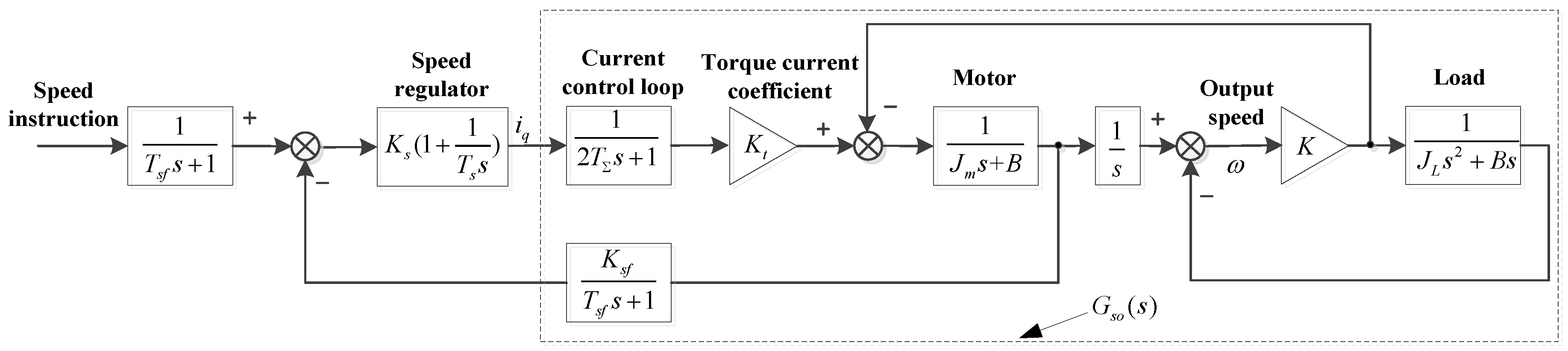
The speed servo system consists of current control loop, servo motor, load, and feedback system. According to the analysis of the component of speed loop, the current closed loop, motor, and speed detection are assumed as first-order systems. Using the PI control algorithm employed as a speed regulator, the speed servo system structure diagram can be obtained in Figure 1.
Where is the proportional gain of current loop. is the integral time constant. is the servo system torque current coefficient. represents the speed feedback coefficient, is the number of detected pulses, represents the resolution of encoder, is the speed detection cycle. is the time constant of current closed-loop approximate system. is the time constant of speed feedback approximate system. is the stiffness coefficient of mechanical transmission. is the conversion coefficient of load friction.
When the impact of resonance on a servo system is ignored, the motor rotor and load object can be assumed as a rigid body and the inertia of the servo system can be expressed as . Where represents motor inertia, is load inertia. The external load torque of the servo system is assumed to be , and the speed-loop-controlled model can be expressed as:
where . Equation (1) can be rearranged into:
where , , , and .
The control time interval is used to discrete Equation (2), and the transfer function of the controlled object of the speed servo system is obtained as follows:
Equation (3) can be rewritten into the following system difference equation for convenience:
where is the speed at time , represents the q axis component of the current. The load torque disturbances can also be described by:
Equation (5) presents that the speed fluctuation caused by changes in load torque is associated with the system inertia and load torque. A small inertia indicates great impacts of the same load torque fluctuations on the speed control process. The system inertia and load torque should be carefully considered during the servo system operation to obtain a stable velocity response. For example, during the movement of the arm of a robot, its inertia is constantly changing. Thus in the CNC machining process, the quality of the processed parts will reduce, which will lead to the change of converted inertia of the feeding axis. When the characteristics of the load object changes, the characteristics of the entire servo system will change. If the system inertia increases, the response of the system will slow down, which is likely to cause system instability and result in climb. On the contrary, if the system inertia decreases, dynamic response will speed up with speed overshoot as well as turbulence.
According to Equations (3)–(5), the relevant parameters of a specific type of servo system are given as follows: of , motor inertia of , and friction coefficient of . We construct system 1 with torque of 1 N·m and load inertia of , system 2 with torque of 1 N·m and load inertia of , and system 3 with torque of 3 N·m and load inertia of to simulate the torque change and disturbance during the operation of the servo system. The rotation inertia and external torque disturbance of the servo system during operation can be considered the jump switches among systems 1, 2, and 3 at different times. The transfer function of the system model can be obtained by taking the above described system 1, 2, and 3 parameters into Equation (1). Using the control time interval to discrete Equation (1), the mathematical model of various servo systems can be obtained according to Equations (4), as shown in Table 1.
3. Servo System Control Strategy Based on Reinforcement Learning
3.1. Strategic Process of Reinforcement Learning
The reinforcement learning framework can be described as the Markov decision process [25]. A limited range of discrete time discount Markov decision processes can be expressed as , where is the state set, is the action set, is the transition probability, is the immediate reward function, is the initial state distribution, is the discount factor, and is a sequence of trajectories. The cumulative return is defined as . The goal of reinforcement learning is to find an optimal strategy that maximizes the reward under this strategy, defined as .
3.1.1. DQN Algorithms
The Monte Carlo method is used to calculate the expectation of return value in the state value function, and the expectation is estimated by a random sample. In calculating the value function, the expectation of the random variable is replaced with the empirical average. Combining with Monte Carlo sampling and dynamic programming methods, the one-step prediction method is used to calculate the current state-value function to obtain the algorithm update formula of Q-learning [26] as follows:
where is the learning rate, represents the discounting factor.
However, the state value of the servo system control is always continuous. The original Q-learning is a learning algorithm based on Q table; therefore, a dimension failure easily occurs in processing the continuous state. DQN can learn value function using a neural network. The network is trained off-policy with samples from a replay buffer to minimize the correlation among samples, and the target neural network is adopted to give consistent targets during temporal difference backups. The target neural network is expressed as . The network that the value function approximates is expressed as , and the loss function is generated as:
3.1.2. Deterministic Policy Gradient Algorithms
The output actions of DQN are discretized and this will result in the failure to find the optimal parameter, or the violent oscillation of the output current. On the basis of the Markov decision process, the single represents the cumulative reward of the track , is defined as the probability of showing the occurrence of a trajectory , and the objective function of reinforcement learning can be expressed as . The goal in reinforcement learning is to learn an optimal parameter that maximizes the expected return from the start distribution, defined as . The objective function is optimized by using the gradient descent ; in the equation, . Further consolidation can be obtained as follows:
The policy gradient algorithm has achieved good results in dealing with the problem of continuous action space. According to the stochastic gradient descent [27], the performance gradient can be expressed as:
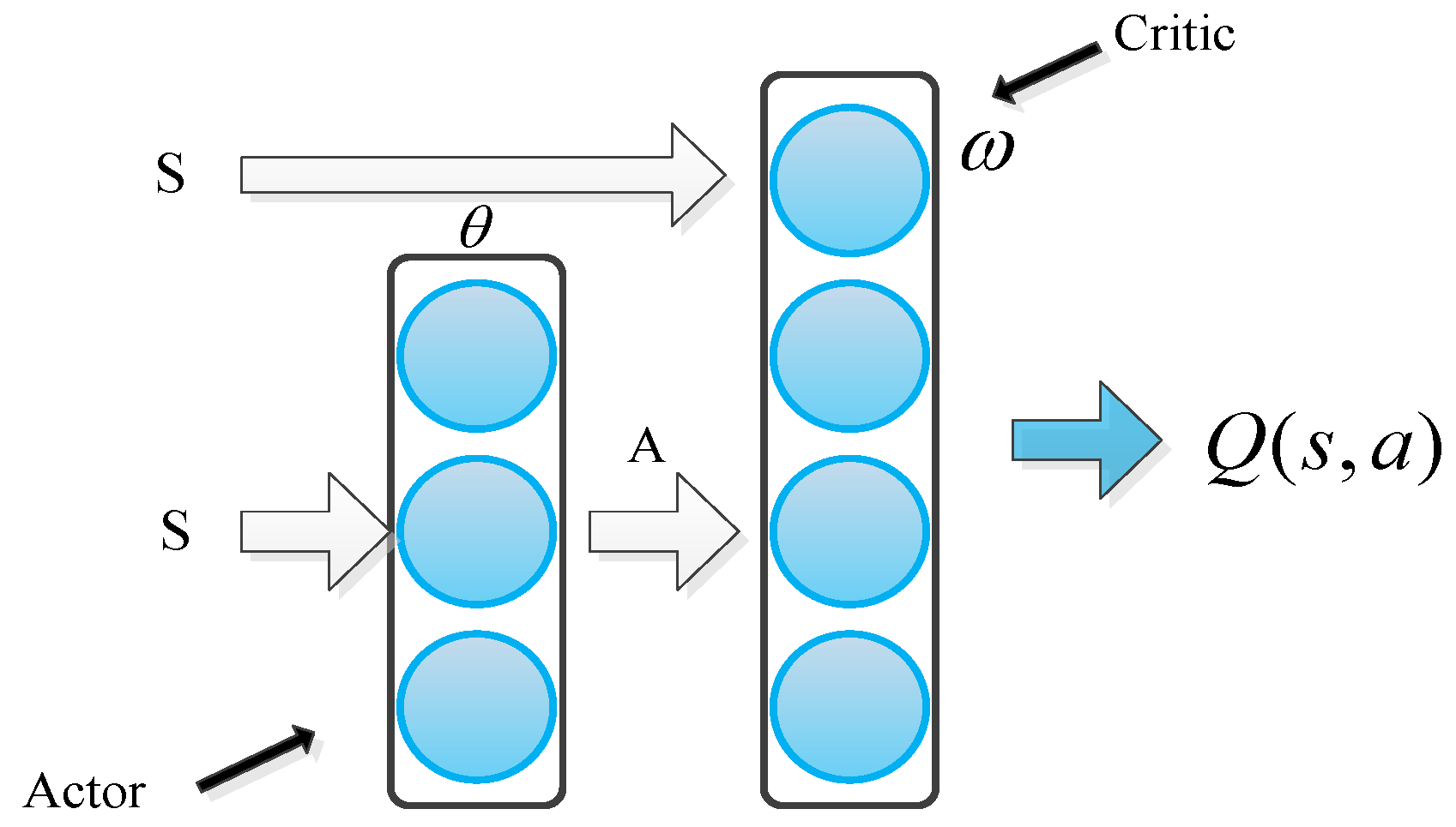
The framework of the actor–critic algorithm based on the idea of the stochastic gradient descent is proposed and widely used [28]. The actor is used to adjust the parameter . The critic approximates the value function , where is the parameter to be approximated. The algorithm structure is shown in Figure 2.
Lillicrap, Hunt, and Pritzel et al. [13] presented an actor–critic, model-free algorithm based on the deterministic policy gradient [27], and the formula of the deterministic policy gradient is:
represents the state behavior strategy. Neural networks are employed to approximate the action-value function and deterministic policy . The updating formula of the DDPG algorithm [13] is obtained as:
3.2. PID Servo System Control Scheme Based on Reinforcement Learning
3.2.1. PID Parameter Tuning Method Based on Reinforcement Learning
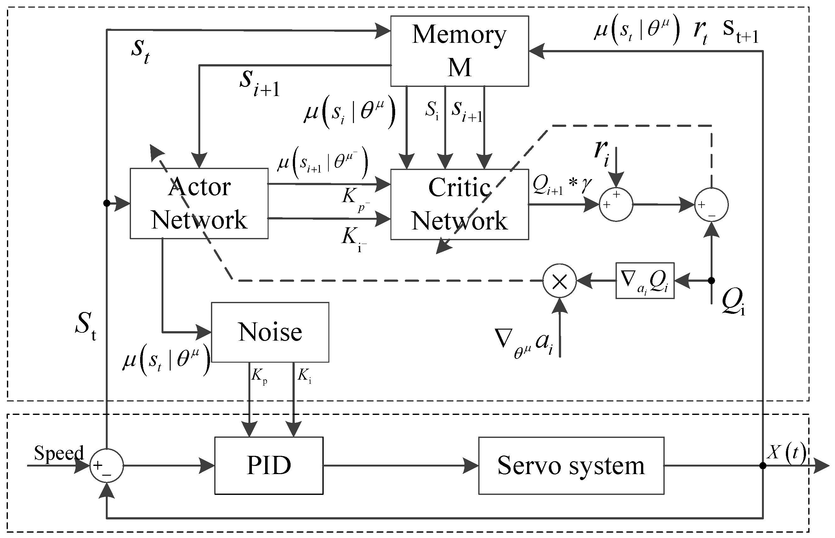
This study uses actor–critic to construct the framework of reinforcement learning agent 1, with a PID servo system as its environment object. The tracking error curve of incentive function is acquired. The deterministic policy gradient algorithm is used to design an action network, and the DQN algorithm is used to design an evaluation network. PID parameter self-tuning is realized. The structure diagram of the adaptive PID control algorithm based on reinforcement learning is shown in Figure 3.
In Figure 3, the upper dotted line frame is an adaptive PID parameter regulator based on reinforcement learning, which is composed of a reinforcement learning agent; the lower dashed box has a PID servo controller and a speed servo system as agent environment interaction objects. is a set of reinforcement learning agent states . is a set of states at the next moment, which is acquired by the interaction of agent 1 and servo environments. , , and denote the angular velocity at the last moment, the current moment, and the next moment of the servo system, respectively. , , and refers to the need to track the signal of the next moment, after two times, and after three times, respectively. , , and are the output error values of the previous moment, at the current time, and at the next moment, respectively. indicates the action selected by the actor evaluation network according to the state , and indicates the action selected by the actor target network according to the state . The PID parameters are a set of action variables to the reinforcement learning agent. The reward function is constructed by the absolute value of the tracking error of the output angle of the servo system. The data are obtained through the interaction of the agent and the servo environment and stored in the memory . The network update data are obtained by memory playback, and the neural networks are trained using Equation (14). The reinforcement learning agent is obtained on the basis of the current state to select the appropriate , and automatic tuning of the parameters of the PID servo system is realized.
3.2.2. Adaptive PID Current Compensation Method Based on Reinforcement Learning
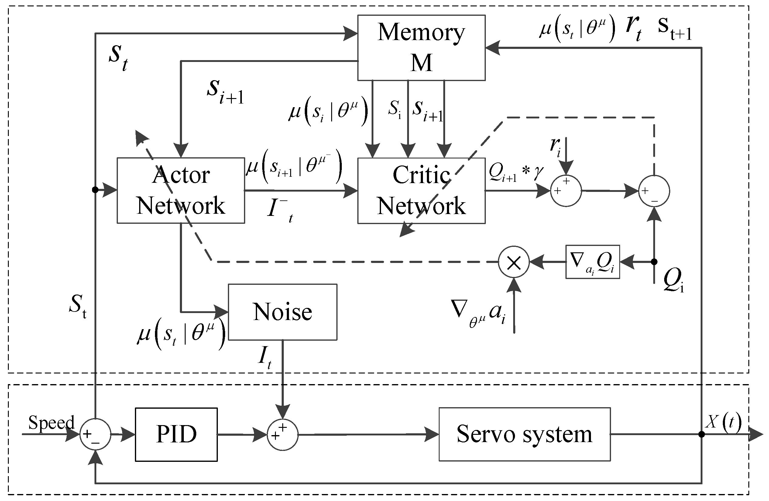
The adaptive PID current compensation agent 2 adopts the same control structure and algorithm as those of agent 1. The adaptive compensation of PID output current is realized. The structure diagram of the adaptive PID control algorithm based on reinforcement learning is shown in Figure 4.
In Figure 4, the upper dotted box is the adaptive current compensator based on reinforcement learning for reinforcement learning agent 2, and the lower dotted box comprises a PID servo controller and a speed servo system as the environment interaction objects of the reinforcement learning agent. The state definition is the same as that of agent 1. The current , as a set of action variables to the reinforcement learning agent, is compensated. The reward function is constructed by the absolute value of the tracking error of the output angle of the servo system. The reinforcement learning agent is achieved on the basis of the current state to select the appropriate , and the adaptive compensation for the PID output current is realized.
3.3. Design Scheme of Reinforcement Learning Agent
3.3.1. Network Design for Actor
Two four-layer neural networks are established on the basis of the deterministic policy gradient algorithm. They are the actor evaluation and target networks, which have the same structures but different functions. The structure of the actor network is shown below:
As illustrated in Figure 5, the actor evaluation network has exactly the same number of neurons and structure as those of the actor target network. The input layer of the actor evaluation network has six neurons, which correspond to six input nodes, namely, for the angular velocity at the last moment, the output error value of the previous moment, the angular velocity at the current moment, the output error value at the current time, the signal needed to track in the next moment, and the signal needed to track after two times, respectively. is a set of reinforcement learning agent state . The action value of the evaluation network is output. The inputs of the actor target network are the current angular velocity , the output error value at the current time, the angular velocity at the next moment after the interaction between action and the environment, the output error value at the next moment, the signal tracked after two times, and the signal tracked after three times. is a set of states at the next moment. The action value of the target network is output. The actor network contains three hidden layers. The first hidden layer comprises 200 neurons, and the activation function in this layer is ReLu6. The second hidden layer also consists of 200 neurons and the activation function is ReLu6. The third hidden layer is composed of 10 neural networks, and the activation function is ReLu. Each layer of neurons uses L2 regularization to prevent overfitting of the neural network.
3.3.2. Network Design for Critic
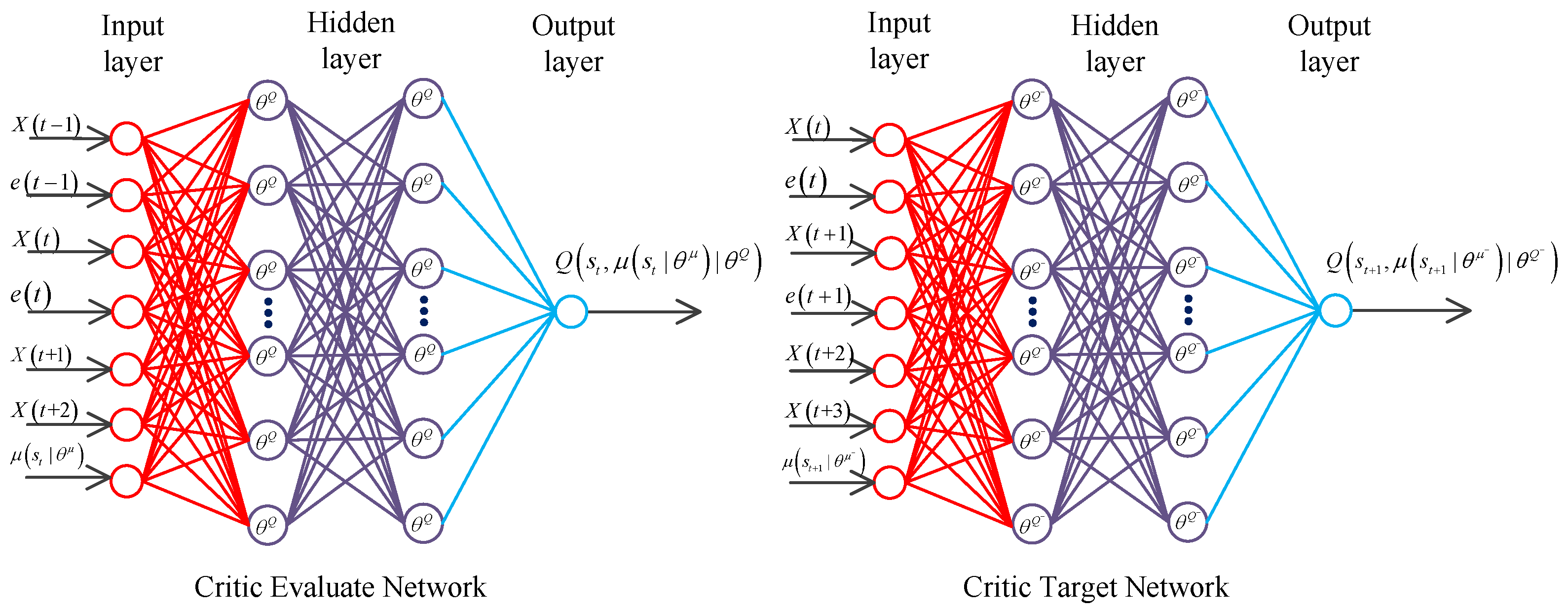
Two four-layer neural networks are established on the basis of the DQN algorithm. They are the critic evaluation and target networks, which have the same structures but different functions. The structure of the critic network is shown below:
As shown in Figure 6, the critic evaluation network has exactly the same number of neurons and structure as those of the critic target network. The input layer of the critic evaluation network has seven neurons, which correspond to seven input nodes, namely, for the angular velocity at the last moment, the output error value of the previous moment, the angular velocity at the current moment, the output error value at the current time, the signal needed to track for the next moment, the signal to track after two times, and the output value of the actor evaluation network. The output layer contains a neuron, which outputs the action-value function . is a set of reinforcement learning agent state . The critic target network also has seven nodes, namely, for the angular velocity at the current moment, the output error value at the current time, the angular velocity at the next moment after the interaction between action and the environment, the output error value at the next moment, the signal to track after two times, the signal to track after three times, and the output value of the actor target network. The critic target network outputs the state-action value function . is a set of states at the next moment. The critic network contains three hidden layers. The first hidden layer comprises 200 neurons, and its activation function is ReLu6.The second hidden layer also consists of 200 neurons, and its activation function is ReLu6. The third hidden layer is composed of 10 neural networks, and its activation function is ReLu. L2 regularization is adopted to prevent overfitting of the neural network.
3.4. Implementation Process of the Adaptive PID Algorithm Based on DDPG Algorithm
In this paper, two types of agents are designed with the same neural network structure. Agent 1 searches for the optimal PID parameters within 0 to 100 range, in order to realize the adaptive tuning of the PID parameters of the speed servo system. The adaptive compensation of PID output current is realized by Agent 2, which further reduces the steady state error.
Agent 1 is designed on the basis of the actor–critic network structure in 3.3. The critic and actor , with weights of and , respectively, are randomly initialized. The target networks and with weights of and , respectively, are randomly initialized. A memory library with capacity is built. The current state is stored. Action is taken. The reward and the next moment state are acquired. The first state is initialized. The action is selected on the basis of the actor evaluation network. The action is performed in the PID servo controller to obtain the return and the next state . The transition is stored in . A random minibatch of transitions from is sampled. is computed, and the critic is updated by minimizing the loss to integrate into Equation (8). The actor network is updated with on the basis of Equation (12). The target network is updated with , .
Agent 2 is designed on the same neural network structure and state set as agent 1. By changing the action space of agent 1, the current compensation of the PID controller is realized and the control performance is further improved. The action is selected on the basis of the actor evaluation network. The same DDPG algorithm with agent 1 is adopted to train the agent 2.
4. Result and Discussion
4.1. Experimental Setup
In the actual application process, the speed servo system instruction is generally trapezoidal or positive rotation. Therefore, only the performances of the servo control system in the two types of instruction cases are analyzed and compared in this study on the basis of system control experiments under the instructions of different amplitudes, frequencies, and rise and fall rates. In the control process of the servo system, PID parameters play a key role in the control performance of the speed servo system. The classic PID (Classic_PID) controller is adopted to compare with the algorithm proposed in this paper. The control parameters turned based on the empirical knowledge from experts are and .
Reinforcement learning agent 1 is constructed on the basis of the method in 3.4.1 to realize automatic tuning of the PID parameters of the servo system. The relevant parameters are set as follows: the capacity of the memory is = 50,000, the actor target network updates the steps by 11,000, and the critic target network updates the steps by 10,000. The action range is [0 to 100]. The learning rate of actor and critic , and the batch size . Gaussian distribution is used to increase noise, and the output value of the neural network is used as the distribution mean. Parameter var 1 is set as the standard deviation, and the initial action noise var 1 = 10. The noise strategy is adjusted dynamically with the increase in learning frequency. Finally, var 1 = 0.01. In this paper, the control precision of the controller is adopted as the control target. In consideration of the limitation of control servo motor current and power consumption in practical engineering, the reward is defined as:
where . Table 1 presents that with the control servo system 1, the tracking amplitude is 1000, the slope absolute value is 13,333.3, the isosceles trapezoidal signal is 0.5 s, the loop iteration is 5000 times, and the environment interaction object is reinforcement learning agent 1. The trained agent model is called MODEL_1.
Reinforcement learning agent 2_1 is constructed on the basis of the method in 3.4.2 to realize the adaptive compensation of PID output current. The optimal control parameters learned by the adaptive PID control algorithm in MODEL_1 are and . The system performance of the fixed PID control structure under these parameters is compared with the control performance of the adaptive current compensation method proposed in this study.
The relevant parameters of the reinforcement agent 2_1 are set as follows: the capacity of the memory is = 50,000, the actor target network updates the steps by 11,000, and the critic target network updates the steps by 10,000. The action range is [−2 to 2]. The learning rate of actor and critic , and the batch size , and the initial action noise var 2 = 2. Finally, var 2 = 0.01. The control output of agent 2_1 needs to compensate the PID current. Therefore, the angular velocity error of PID control is constructed to build the reward function , and the reward is defined as:
where . The environment interaction object of agent 1 is adopted to the reinforcement learning agent 2_1. Eight hundred episodes are trained to acquire the agent model, called MODEL_2.
Agent 2_2 is constructed on the basis of the structure of agent 2_1. Agent 2_2 changes the relevant parameters on the basis of agent 2_1 as follows: the memory is changed to , the capacity of the memory is , the actor target network updates the steps by 1100, the critic target network updates the steps by 1000, and the remaining indicators are unchanged by agent 2_2. The compensation tracking amplitude is 10, and the frequency is 100 Hz sinusoidal signal. Four thousand episodes are trained to acquire the agent model MODEL_3.
The system models of system inertia mutation and external torque disturbance are tested to verify the adaptability of the proposed adaptive control strategy based on the adaptive speed servo system of reinforcement learning in this study. The performance of the proposed method is quantitatively analyzed with velocity tracking curve rendering, velocity tracking error value, and Integral of Absolute Error (IAE) index value.
4.2. Experimental Results
Test case #1
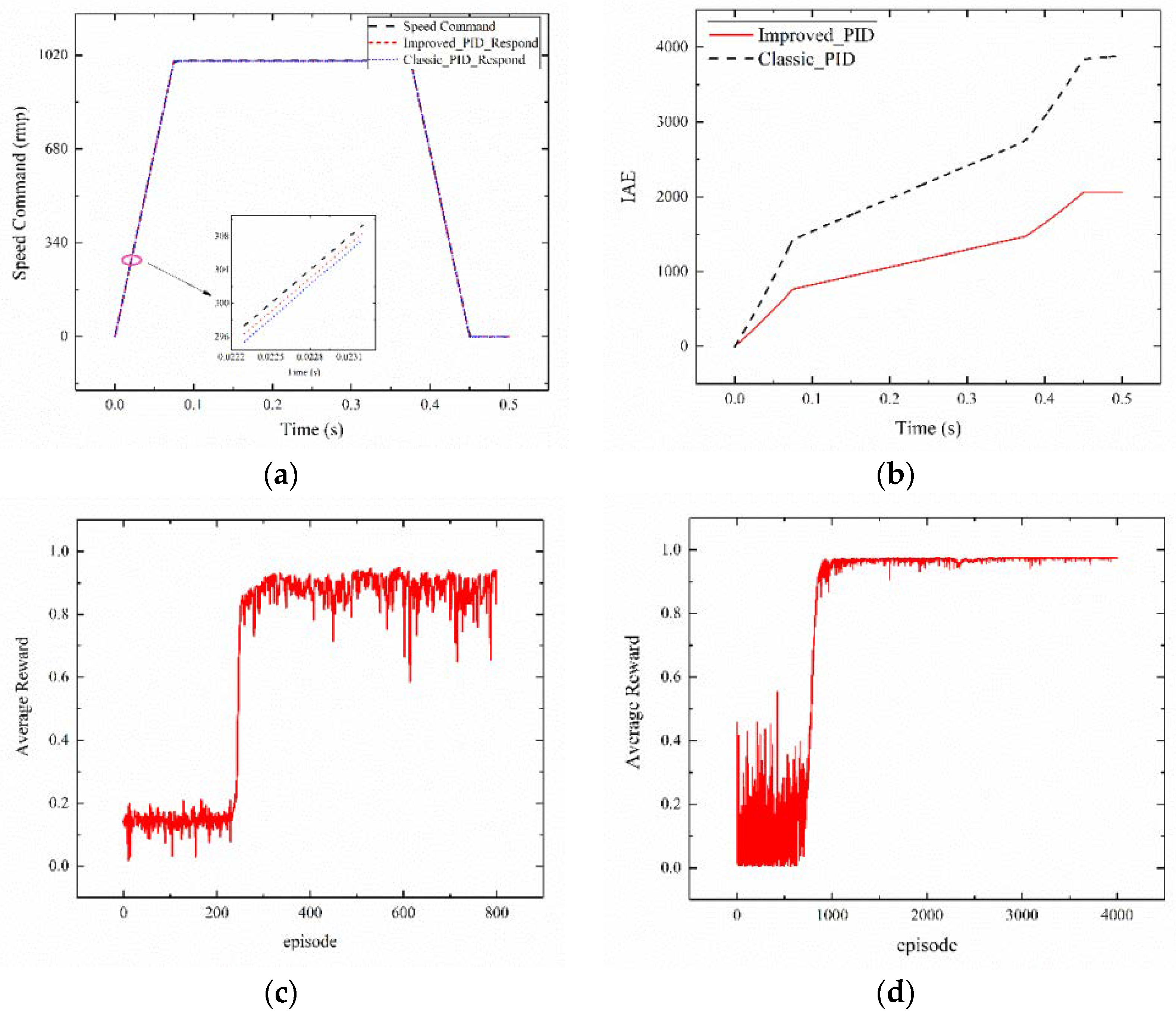
The following figure shows the data of the successful training of each model. The performance test of MODEL_1 is shown in Figure 7a, in which the tracking amplitude of agent 1 is 1000, the absolute value of the slope is 13,333.3, and the isosceles trapezoid tracking effect presents an inconsiderable error. The reinforcement learning output action values of Kp, Ki present a straight line. The optimal control parameters are and . It can be seen from the Figure 7b that the improved PID (Improved_PID) with good parameters can achieve better control performance than Classic_PID. Figure 7c indicates that 800 episode values are trained to acquire the average reward for agent 2_1. The training is started by exploring a large degree, where in the average reward value is very low. As the training steps increase, the average reward increases gradually, and MODEL_2 eventually converges. Figure 7d depicts the average reward of agent 2_2 when training 4000 episode values. The average reward eventually increases and tends to be stable. The correctness and effectiveness of the agent model of the proposed method in this study are verified according to the above results.
Test case #2
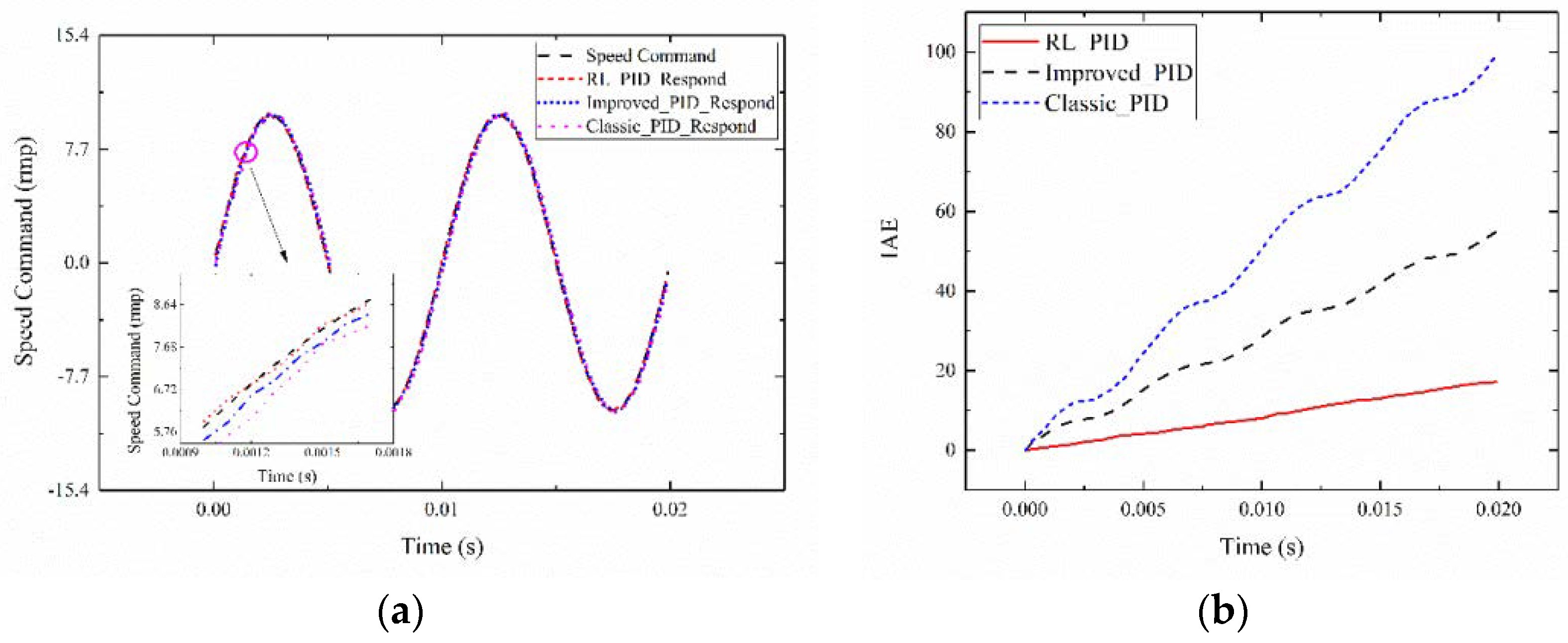
The tracking command signal of the setting system is set with the amplitude value of 1000, the slope absolute value of 13,333.3 isosceles trapezoid signal, amplitude of 0.1, zero mean, variance of 1, and random white Gaussian noise signal. When tracking 0.5 s, system 1 is selected as the servo system in the tracking process. The reinforcement learning adaptive PID current compensation method is compared with PID control. The MODEL_2 control and the performance comparison of the PID approaches are shown in Figure 8.
Figure 8a presents the tracking effect diagram of 0.50 s for the reinforcement learning adaptive PID current compensation method. A good tracking performance is obtained. The circle-part amplification is shown in the figure. Agent 2_1 tracking effect (RL_PID) is compared with Classic_PID and Improved_PID. In the absence of external disturbances, the proposed method can rapidly and accurately track the command signal, and the Classic_PID control structure produces a large tracking error. The control performance of Improved_PID is between Classic_PID and RL_PID. The parameter tuning method proposed in this paper can achieve better control performance than the Classic_PID. Figure 8b depicts the IAE index for RL_PID, Improved_PID, and Classic_PID. The IAE of the reinforcement learning adaptive PID control algorithm is smaller than that of the PID algorithm under the condition of the same system. The results prove that the proposed control strategy is feasible in tracking trapezoidal signal and can achieve a good control performance.
Test case #3
The tracking command signal of the setting system has an amplitude value of 2000, aslope absolute value of 26,666.6 isosceles trapezoid signal, an amplitude of 0.1, zero mean, variance of 1, and a random white Gaussian noise signal. When tracking 0.5 s, system 1 is selected as the servo system. The inertia and moment disturbance of the random system are added between 0.075 and 0.375 s. The reinforcement learning adaptive PID current compensation method (RL_PID) is compared with Improved_PID control, and Classic_PID. The MODEL_2 control and the performance comparison of the PID approaches are shown in Figure 9.
Figure 9a presents the tracking effect diagram of 0.50 s for the reinforcement learning adaptive PID current compensation method. A good tracking performance is observed. The circle-part amplification is shown in the figure. Agent 2_1 tracking effect (RL_PID) is compared with Improved_PID and Classic_PID. The proposed method follows the signal amplitude. The slope with changed circumstances shows a better tracking effect than that of the Improved_PID and Classic_PID. This method is verified to have good adaptability. Figure 9b shows a schematic of the control system of the adaptive PID and PID control algorithms, where 0 represents system 1, 1 represents system 2, and 2 represents system 3. Figure 9c depicts the comparison chart of the reinforcement learning adaptive PID control algorithm and the PID control algorithm IAE. The IAE value of the reinforcement learning adaptive PID control algorithm is always less than that of the PID algorithm under the same system. The image above Figure 9d shows the comparison diagram of the RL_PID, Improved_PID and Classic_PID tracking error. When the system changes, the tracking error of the reinforcement learning is less than that of the Improved_PID and Classic_PID. It can be obtained from the figure that the PID controller after turning the parameter of the agent 1 is better than the classical PID controller to reduce the tracking error caused by the mutation of inertia. Current compensation in the PID controller after turning parameters can reduce the error further. The figure below Figure 9d shows the current value of the RL_PID based on reinforcement learning output. When the system undergoes mutation, the output current value of the reinforcement learning (RL_PID_RL) in adaptive PID based on reinforcement learning and the value of PID (RL_PID_PID) in adaptive PID based on reinforcement learning change to adapt to the system. The results prove that the proposed control strategy in tracking trapezoidal signal amplitude, slope change, system inertia, and torque under the condition of random mutation is still better than Improved_PID and Classic_PID. The applicability and superiority of the proposed method are verified.
Test case #4
The tracking command signal is set with a signal amplitude of 10, a frequency of 100 Hz sinusoidal signal, an amplitude of 0.1, zero mean, variance of 1, and random white Gaussian noise signal. When tracking 0.02 s, system 1 is selected as the servo system, and agent 2_2 is tested. The reinforcement learning adaptive PID current compensation method is compared with Improved_PID control and Classic_PID control. The MODEL_3 control and the performance comparison of Improved_PID and Classic_PID are shown in Figure 10.
Figure 10a is the tracking effect diagram of 0.02 s for the reinforcement learning adaptive PID current compensation method. A good tracking performance is yielded, and the circle-part amplification is shown in the figure. Agent 2_2 tracking effect is compared with Improved_PID and Classic_PID. In the absence of external disturbances, the proposed method can rapidly and accurately track the command signal, and the Classic_PID control structure produces a large tracking error. The control performance of Improved_PID with good parameters is better than that of Classic_PID, which verifies that the parameters searched by the reinforcement learning agent 1 can still be applied when the tracking signal type changes. Figure 10b shows the IAE index for the reinforcement learning adaptive PID control algorithm, Improved_PID and Classic_PID control algorithm. The IAE of the reinforcement learning adaptive PID control algorithm is smaller than that of the Improved_PID algorithm and Classic_PID algorithm under the condition of the same system. The results confirm that the control strategy proposed in this study is feasible to track sinusoidal signal and can obtain a good control performance.
Test case #5
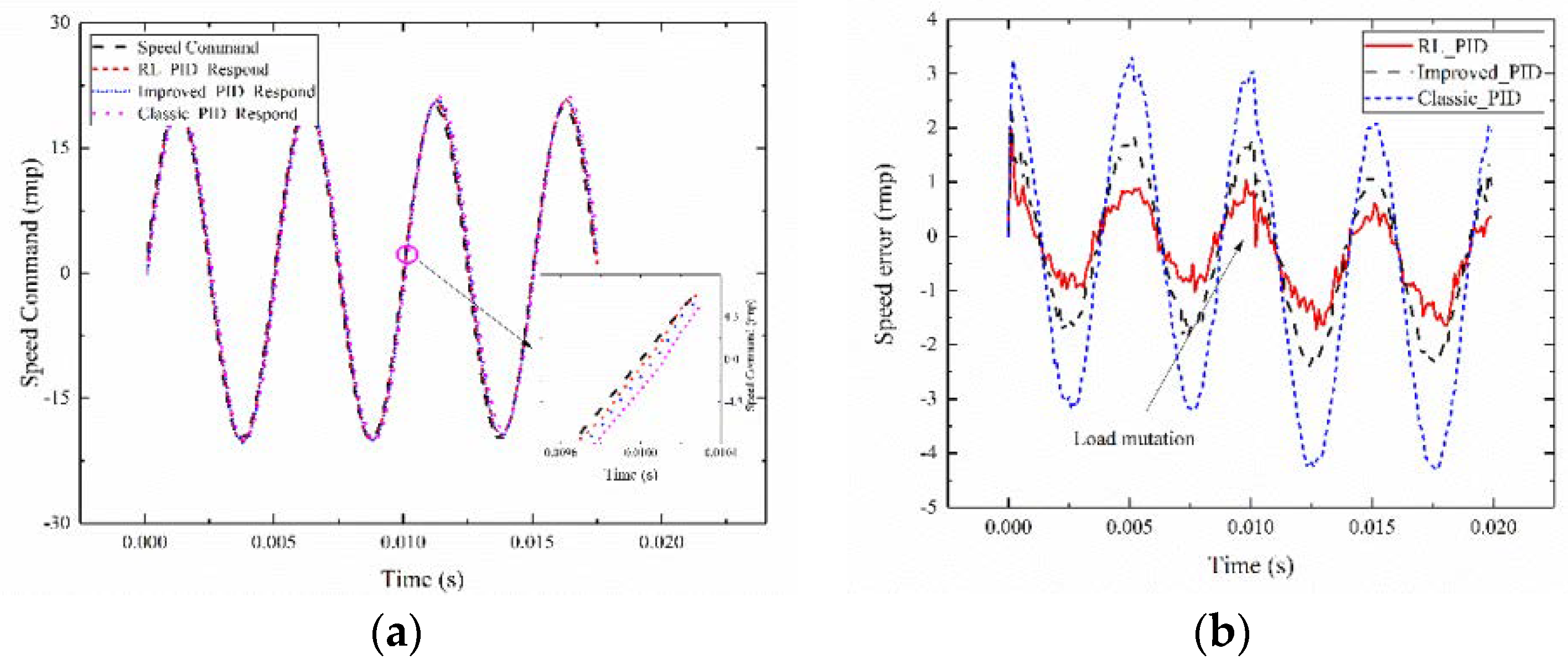
The tracking command signal is set with a signal amplitude of 20, a frequency of 200 Hz sinusoidal signal, an amplitude of 0.1, zero mean, variance of 1, and random white Gaussian noise signal. When tracking 0.02 s, system 1 is selected as the servo system. The torque mutation system is switched to system 3 at 0.01 s, and agent 2_2 is tested. The reinforcement learning adaptive PID current compensation method is compared with Improved_PID and Classic_PID. The MODEL_3 control and the performance comparison of the PID approaches are shown in Figure 11.
Figure 11a presents the tracking effect diagram of 0.02 s for the reinforcement learning adaptive PID current compensation method. A good tracking performance is obtained, and the circle-part amplification is shown in the figure. From the comparison between the tracking effect (RL_PID), Improved_PID and Classic_PID tracking effect, the tracking effect of the proposed method is still better than that of the no current compensation PID control structure. Figure 11b is the error graph of the adaptive PID, Improved_PID, and Classic_PID control algorithms. The error value of the adaptive PID control algorithm is significantly smaller than that of the Improved_PID algorithm and the Classic_PID algorithm under the same system. The Improved_PID has a better PID parameter that can achieve a smaller tracking error than Classic_PID when the load is a mutation. The results prove that the presented control strategy under the condition of torque mutation has a better tracking performance than that of Improved_PID and Classic_PID. The applicability and superiority of the proposed method are verified.
Test case #6
The proposed control strategy based on reinforcement learning is compared with fixed parameter PID control performance of servo system structure under the circumstances of different signal types, signal amplitudes, torques, and inertia mutations, with its IAE as the evaluation index. For the system with random mutation, random system inertia is added, and the torque disturbance ranges from 0.075 s to 0.375 s. For the system with inertia mutation, 0.01 s switch to system 2 is required. For the system with load mutation, 0.01 s system to switch to system 3 is needed. The results are shown in Table 2, Table 3, Table 4 and Table 5.
According to the experimental results in different velocity commands and complex disturbances and inertia change under such circumstances, the IAE index of the method proposed in this study is less than the IAE index value of the fixed parameter PID control system. The proposed method has a better control performance than the PID control structure with fixed parameters and has good adaptability. In addition, the proposed PID parameter tuning method based on deep reinforcement learning can search better control parameters, create the fixed parameter PID control system under the condition of the system of inertia, and load mutations that can obtain better control performance than classic PID.
5. Conclusions
In this study, we design a reinforcement learning agent to automatically control the parameters of a speed servo system. The agent establishes the networks of action and critic functions on the basis of the DDPG algorithm. The action network realizes the optimal approximation of the strategy. The critic network realizes the optimal approximation of the value function and adopts the strategies of memory playback, parameter freezing, and noise dynamic adjustment to improve the convergence speed of neural networks. The tuning parameters of the servo system are obtained, and the same reinforcement learning intelligent structure is adopted to enhance the control accuracy.
The use of reinforcement learning cannot only make the control parameters of the servo system have fast and accurate tuning, but also can perform current online compensation on the basis of the state of the servo system. The system can effectively overcome the influences of external factors. This study proposes a servo system control strategy based on reinforcement learning in different types of instructions, torque disturbances, and inertia cases. A satisfactory performance of the control system is obtained. The experimental results demonstrate the effectiveness and robustness of the proposed method. In this paper, the tuning of PID parameters of the servo system and the compensation of current are two agents. Multi-task learning may solve this problem and this will be the topic of a future work. In addition, we find that L2 regularization can improve the generalization ability of reinforcement learning agents. The contributions in this paper will be beneficial to the application of deep reinforcement learning in a servo system.
Author Contributions
P.C. contributed to the conception of the reported research and helped revise the manuscript. Z.H. contributed significantly to the design and conduct of the experiment and the analysis of results, as well as contributed to the writing of the manuscript. C.C. and J.X. helped design the experiments and perform the analysis with constructive discussions.
Acknowledgments
This research is supported by the National Natural Science Foundation of China (61663011) and the postdoctoral fund of Jiangxi Province (2015KY19).
Conflicts of Interest
The authors declare no conflicts of interest.
References
- Zheng, S.; Tang, X.; Song, B.; Ye, B. Stable adaptive PI control for permanent magnet synchronous motor drive based on improved JITL technique. ISA Trans. 2013, 52, 539–549. [Google Scholar] [CrossRef] [PubMed]
- Roy, P.; Roy, B.K. Fractional order PI control applied to level control in coupled two tank MIMO system with experimental validation. Control Eng. Pract. 2016, 48, 119–135. [Google Scholar] [CrossRef]
- Ang, K.H.; Chong, G.; Li, Y. PID control system analysis, design, and technology. IEEE Trans. Control Syst. Technol. 2005, 13, 559–576. [Google Scholar] [CrossRef]
- Sekour, M.; Hartani, K.; Draou, A.; Ahmed, A. Sensorless Fuzzy Direct Torque Control for High Performance Electric Vehicle with Four In-Wheel Motors. J. Electr. Eng. Technol. 2013, 8, 530–543. [Google Scholar] [CrossRef]
- Zhang, X.; Sun, L.; Zhao, K.; Sun, L. Nonlinear Speed Control for PMSM System Using Sliding-Mode Control and Disturbance Compensation Techniques. IEEE Trans. Power Electron. 2012, 28, 1358–1365. [Google Scholar] [CrossRef]
- Dang, Q.D.; Vu, N.T.T.; Choi, H.H.; Jung, J.W. Neuro-Fuzzy Control of Interior Permanent Magnet Synchronous Motors. J. Electr. Eng. Technol. 2013, 8, 1439–1450. [Google Scholar] [CrossRef]
- El-Sousy, F.F.M. Adaptive hybrid control system using a recurrent RBFN-based self-evolving fuzzy-neural-network for PMSM servo drives. Appl. Soft Comput. 2014, 21, 509–532. [Google Scholar] [CrossRef]
- Jezernik, K.; Korelič, J.; Horvat, R. PMSM sliding mode FPGA-based control for torque ripple reduction. IEEE Trans. Power Electron. 2012, 28, 3549–3556. [Google Scholar] [CrossRef]
- Jung, J.W.; Leu, V.Q.; Do, T.D.; Kim, E.K.; Choi, H.H. Adaptive PID Speed Control Design for Permanent Magnet Synchronous Motor Drives. IEEE Trans. Power Electron. 2014, 30, 900–908. [Google Scholar] [CrossRef]
- Mnih, V.; Kavukcuoglu, K.; Silver, D.; Graves, A.; Antonoglou, I.; Wierstra, D.; Riedmiller, M. Playing Atari with Deep Reinforcement Learning. Comput. Sci. 2013. Available online: https://arxiv.org/pdf/1312.5602v1.pdf (accessed on 3 May 2018).
- Mnih, V.; Kavukcuoglu, K.; Silver, D.; Rusu, A.A.; Veness, J.; Bellemare, M.G.; Graves, A.; Riedmiller, M.; Fidjeland, A.K.; Ostrovski, G.; et al. Human-level control through deep reinforcement learning. Nature 2015, 518, 529–533. [Google Scholar] [CrossRef] [PubMed]
- Silver, D.; Huang, A.; Maddison, C.J.; Guez, A.; Sifre, L.; van den Driessche, G.; Schrittwieser, J.; Antonoglou, I.; Panneershelvam, V.; Lanctot, M.; et al. Mastering the game of Go with deep neural networks and tree search. Nature 2016, 529, 484–489. [Google Scholar] [CrossRef] [PubMed]
- Lillicrap, T.P.; Hunt, J.J.; Pritzel, A.; Heess, N.; Erez, T.; Tassa, Y.; Silver, D.; Wierstra, D. Continuous control with deep reinforcement learning. Comput. Sci. 2015, 8, A187. Available online: http://xueshu.baidu.com/s?wd=paperuri%3A%283752bdb69e8a3f4849ecba38b2b0168f%29&filter=sc_long_sign&tn=SE_xueshusource_2kduw22v&sc_vurl=http%3A%2F%2Farxiv.org%2Fabs%2F1509.02971&ie=utf-8&sc_us=1138439324812222606 (accessed on 3 May 2018).
- Jiang, H.; Zhang, H.; Luo, Y.; Wang, J. Optimal tracking control for completely unknown nonlinear discrete-time Markov jump systems using data-based reinforcement learning method. Neurocomputing 2016, 194, 176–182. [Google Scholar] [CrossRef]
- Carlucho, I.; Paula, M.D.; Villar, S.; Acosta, G.G. Incremental Q-learning strategy for adaptive PID control of mobile robots. Expert Syst. Appl. 2017, 80, 183–199. [Google Scholar] [CrossRef]
- Yu, R.; Shi, Z.; Huang, C.; Li, T.; Ma, Q. Deep reinforcement learning based optimal trajectory tracking control of autonomous underwater vehicle. In Proceedings of the 2017 36th Chinese Control Conference (CCC), Dalian, China, 26–28 July 2017; IEEE: Piscataway, NJ, USA, 2017; pp. 4958–4965. [Google Scholar] [CrossRef]
- Zhao, H.; Wang, Y.; Zhao, M.; Sun, C.; Tan, Q. Application of Gradient Descent Continuous Actor-Critic Algorithm for Bilateral Spot Electricity Market Modeling Considering Renewable Power Penetration. Algorithms 2017, 10, 53. [Google Scholar] [CrossRef]
- Hu, Y.; Li, W.; Xu, K.; Zahid, T.; Qin, F.; Li, C. Energy Management Strategy for a Hybrid Electric Vehicle Based on Deep Reinforcement Learning. Appl. Sci. 2018, 8, 187. [Google Scholar] [CrossRef]
- Lin, C.H. Composite recurrent Laguerre orthogonal polynomials neural network dynamic control for continuously variable transmission system using altered particle swarm optimization. Nonlinear Dyn. 2015, 81, 1219–1245. [Google Scholar] [CrossRef]
- Liu, Y.J.; Tong, S. Adaptive NN tracking control of uncertain nonlinear discrete-time systems with nonaffine dead-zone input. IEEE Trans. Cybern. 2017, 45, 497–505. [Google Scholar] [CrossRef] [PubMed]
- Dos Santos Mignon, A.; da Rocha, R.L.A. An Adaptive Implementation of ε-Greedy in Reinforcement Learning. Procedia Comput. Sci. 2017, 109, 1146–1151. [Google Scholar] [CrossRef]
- Plappert, M.; Houthooft, R.; Dhariwal, P.; Sidor, S.; Chen, R.Y.; Chen, X.; Asfour, T.; Abbeel, P.; Andrychowicz, M. Parameter Space Noise for Exploration. Comput. Sci. 2017. Available online: http://xueshu.baidu.com/s?wd=paperuri%3A%28c8411e5bc5e651d776e9d4997604cc3e%29&filter=sc_long_sign&tn=SE_xueshusource_2kduw22v&sc_vurl=http%3A%2F%2Farxiv.org%2Fabs%2F1706.01905&ie=utf-8&sc_us=8746754823928227025 (accessed on 3 May 2018).
- Nigam, K. Using maximum entropy for text classification. In Proceedings of the IJCAI-99 Workshop on Machine Learning for Information Filtering, Stockholm, Sweden, 1 August 1999; pp. 61–67. Available online: http://www.kamalnigam.com/papers/maxent-ijcaiws99.pdf (accessed on 3 May 2018).
- Ng, A.Y. Feature selection, L1 vs. L2 regularization, and rotational invariance. In Proceedings of the Twenty-First International Conference on Machine Learning, Banff, AB, Canada, 4–8 June 2004; ACM: New York, NY, USA, 2004; p. 78. Available online: http://www.yaroslavvb.com/papers/ng-feature.pdf (accessed on 3 May 2018).
- Monahan, G.E. A Survey of Partially Observable Markov Decision Processes: Theory, Models, and Algorithms. Manag. Sci. 1982, 28, 1–16. [Google Scholar] [CrossRef]
- Sutton, R.S.; Barto, A.G. Reinforcement Learning: An Introduction; MIT Press: Cambridge, MA, USA, 1998; Available online: http://www.umiacs.umd.edu/~hal/courses/2016F_RL/RL9.pdf (accessed on 3 May 2018).
- Silver, D.; Lever, G.; Heess, N.; Thomas, D.; Wierstra, D.; Riedmiller, M. Deterministic policy gradient algorithms. In Proceedings of the International Conference on International Conference on Machine Learning, Beijing, China, 21–26 June 2014; pp. 387–395. Available online: http://www0.cs.ucl.ac.uk/staff/d.silver/web/Applications_files/deterministic-policy-gradients.pdf (accessed on 3 May 2018).
- Konda, V.R.; Tsitsiklis, J.N. Actor-critic algorithms. SIAM J. Control Optim. 2002, 42, 1143–1166. Available online: http://web.mit.edu/jnt/OldFiles/www/Papers/C.-99-konda-NIPS.pdf (accessed on 3 May 2018). [CrossRef]
Figure 1.
Diagram of the speed servo system structure.

Figure 2.
Diagram of the actor–critic algorithm structure.

Figure 3.
Adaptive proportional–integral–derivative (PID) control structure diagram based on reinforcement learning agent 1.
Figure 3.
Adaptive proportional–integral–derivative (PID) control structure diagram based on reinforcement learning agent 1.

Figure 4.
Adaptive PID current compensation control structure diagram based on reinforcement learning agent 2.
Figure 4.
Adaptive PID current compensation control structure diagram based on reinforcement learning agent 2.

Figure 5.
Structure diagram of the actor network.
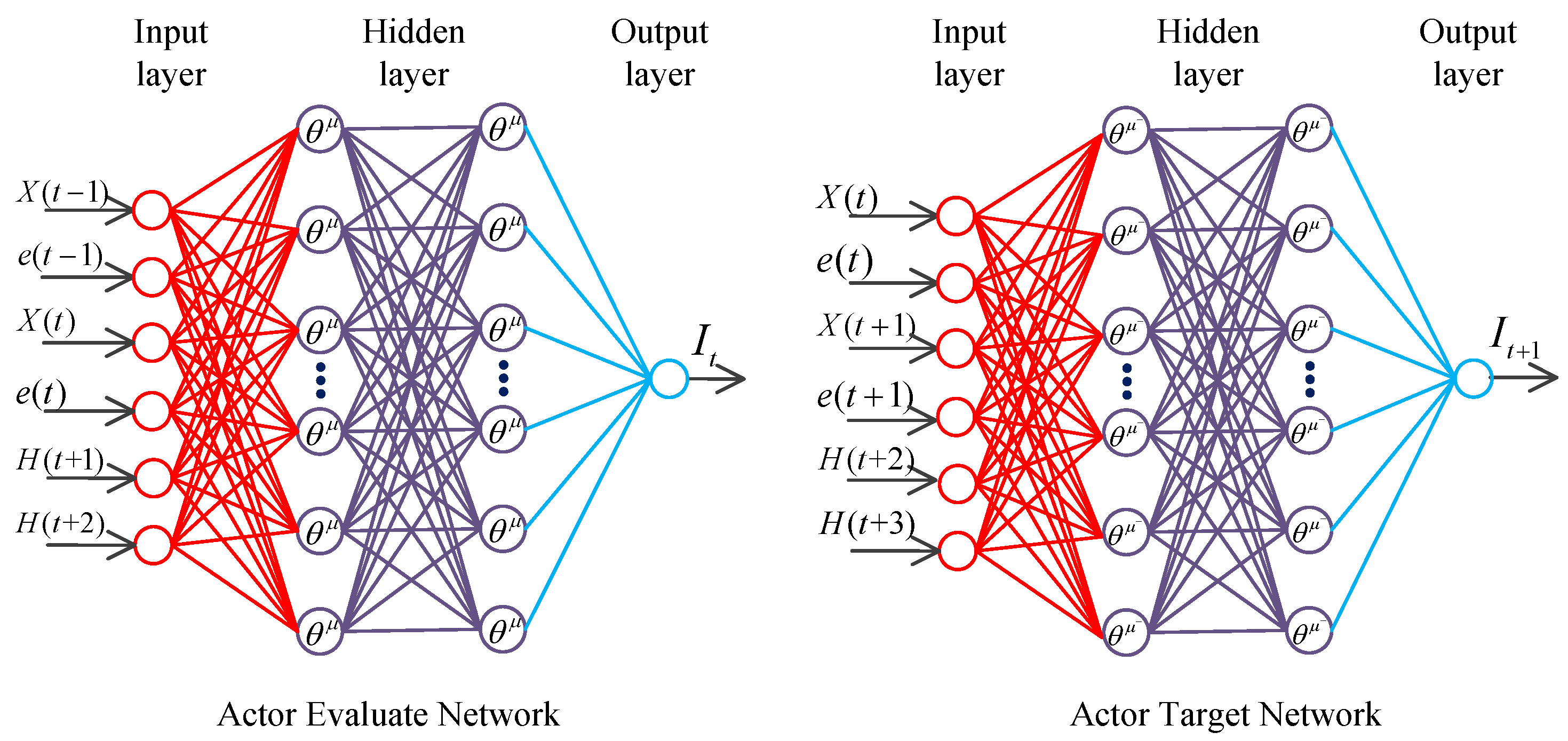
Figure 6.
Structure diagram of the critic network.

Figure 7.
Result of test case #1. (a) Agent 1 tracking renderings; (b) Integral of absolute error (IAE) index comparison diagram; (c) Average reward value of agent 2_1; (d) Average reward value of agent 2_2.
Figure 7.
Result of test case #1. (a) Agent 1 tracking renderings; (b) Integral of absolute error (IAE) index comparison diagram; (c) Average reward value of agent 2_1; (d) Average reward value of agent 2_2.

Figure 8.
Result of test case #2. (a) Tracking signal comparison diagram; (b) IAE index comparison diagram.
Figure 8.
Result of test case #2. (a) Tracking signal comparison diagram; (b) IAE index comparison diagram.
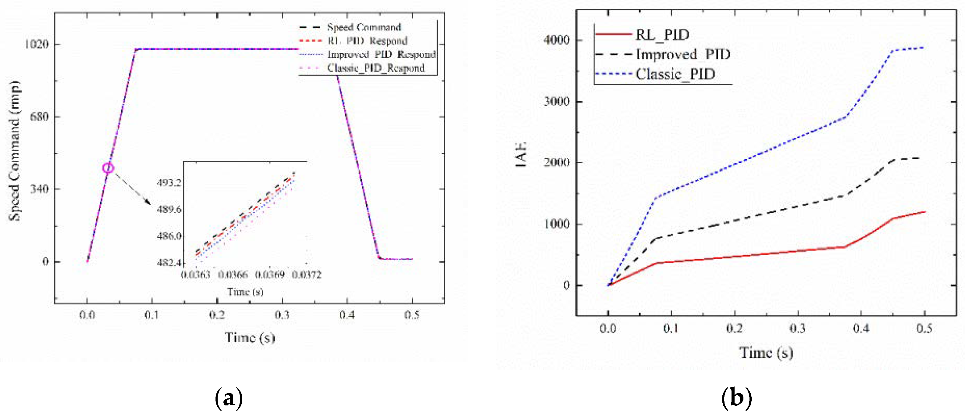
Figure 9.
Result of test case #3 (a) Tracking signal comparison diagram; (b) System selection chart; (c) IAE index comparison diagram; (d) Agent 2_1 output current value and tracking error graph.
Figure 9.
Result of test case #3 (a) Tracking signal comparison diagram; (b) System selection chart; (c) IAE index comparison diagram; (d) Agent 2_1 output current value and tracking error graph.
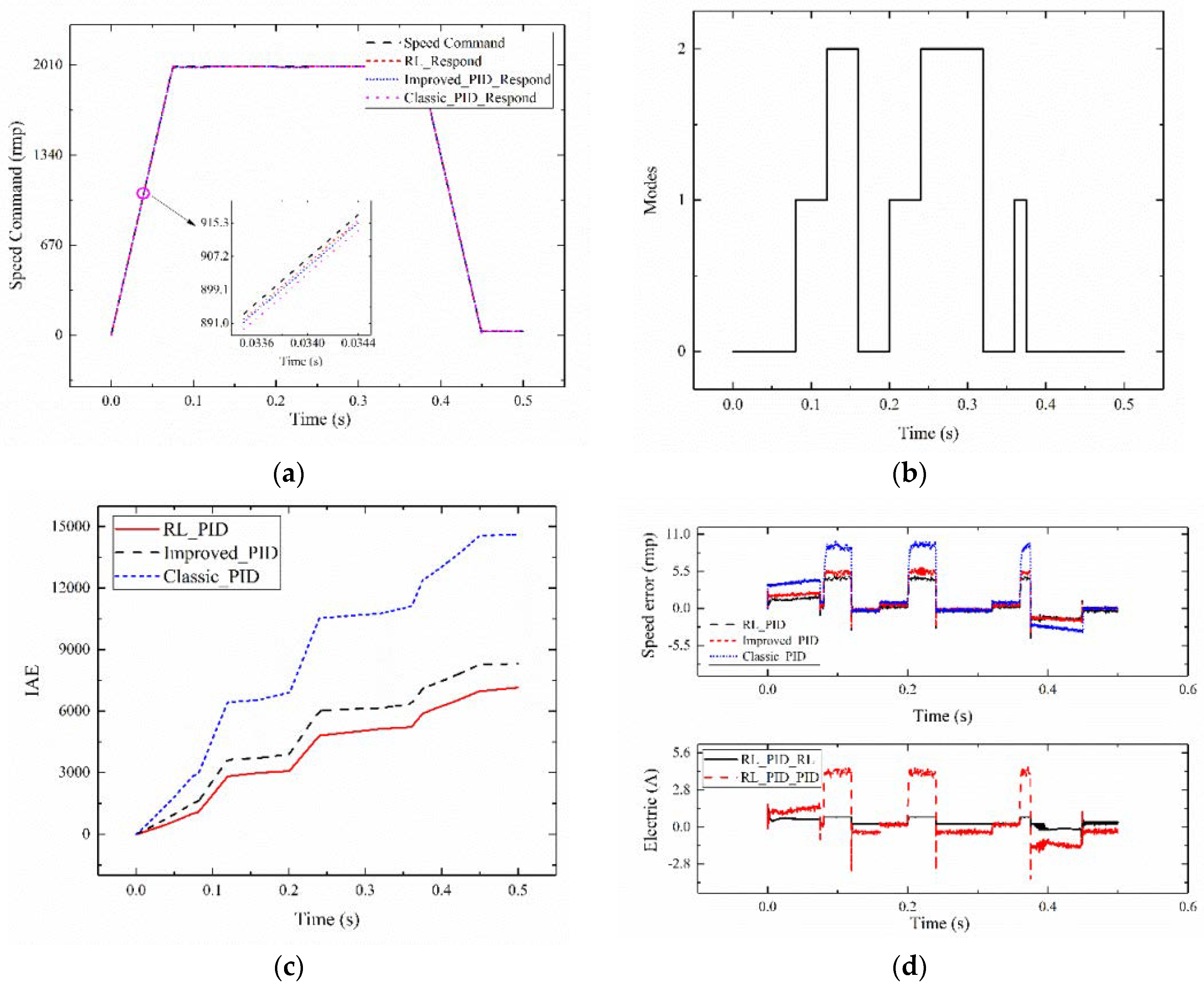
Figure 10.
Result of test case #4. (a) Tracking signal comparison diagram; (b) IAE index comparison diagram.
Figure 10.
Result of test case #4. (a) Tracking signal comparison diagram; (b) IAE index comparison diagram.

Figure 11.
Result of test case #5. (a) Tracking signal comparison diagram; (b) Tracking error comparison diagram.
Figure 11.
Result of test case #5. (a) Tracking signal comparison diagram; (b) Tracking error comparison diagram.


Table 1.
Servo system model.
| System | Differential Equation Expression of The Mathematical Model |
|---|---|
| System 1 | |
| System 2 | |
| System 3 |
Table 2.
Amplitude value with 1000 slope 13,333.3 isosceles trapezoid tracking signal under 0.5 s RL_PID, Improved_PID and Classic_PID IAE indicator table.
Table 2.
Amplitude value with 1000 slope 13,333.3 isosceles trapezoid tracking signal under 0.5 s RL_PID, Improved_PID and Classic_PID IAE indicator table.
| System | RL_PID | Improved_-PID | Classic_PID |
|---|---|---|---|
| System 1 | 1199.56 | 2087.81 | 3883.61 |
| system with random mutation | 4000.01 | 5444.85 | 8017.54 |
Table 3.
Amplitude value with 2000 slope 26,666.6 isosceles trapezoid tracking signal under 0.5 s RL_PID, Improved_PID and Classic_PID IAE indicator table.
Table 3.
Amplitude value with 2000 slope 26,666.6 isosceles trapezoid tracking signal under 0.5 s RL_PID, Improved_PID and Classic_PID IAE indicator table.
| System | RL_PID | Improved_PID | Classic_PID |
|---|---|---|---|
| System 1 | 2937.40 | 4144.64 | 7705.06 |
| system with random mutation | 7144.29 | 8307.17 | 14,608.11 |
Table 4.
Amplitude with 10 frequency 100 sinusoidal tracking signal under 0.02 s RL_PID, Improved_PID and Classic_PID IAE indicator table.
Table 4.
Amplitude with 10 frequency 100 sinusoidal tracking signal under 0.02 s RL_PID, Improved_PID and Classic_PID IAE indicator table.
| System | RL_PID | Improved_PID | Classic_PID |
|---|---|---|---|
| System 1 | 17.126 | 54.412 | 99.760 |
| system with inertia mutation | 199.045 | 271.327 | 427.420 |
| system with load mutation | 60.300 | 89.819 | 166.420 |
Table 5.
Amplitude with 20 frequency 200 sinusoidal tracking signal under 0.02 s RL_PID, Improved_PID and Classic_PID IAE indicator table.
Table 5.
Amplitude with 20 frequency 200 sinusoidal tracking signal under 0.02 s RL_PID, Improved_PID and Classic_PID IAE indicator table.
| System | RL_PID | Improved_PID | Classic_PID |
|---|---|---|---|
| System 1 | 112.418 | 217.766 | 403.680 |
| system with inertia mutation | 827.467 | 952.202 | 1278.677 |
| system with load mutation | 129.000 | 226.029 | 417.880 |
© 2018 by the authors. Licensee MDPI, Basel, Switzerland. This article is an open access article distributed under the terms and conditions of the Creative Commons Attribution (CC BY) license (http://creativecommons.org/licenses/by/4.0/).
Share and Cite
MDPI and ACS Style
Chen, P.; He, Z.; Chen, C.; Xu, J. Control Strategy of Speed Servo Systems Based on Deep Reinforcement Learning. Algorithms 2018, 11, 65. https://doi.org/10.3390/a11050065
AMA Style
Chen P, He Z, Chen C, Xu J. Control Strategy of Speed Servo Systems Based on Deep Reinforcement Learning. Algorithms. 2018; 11(5):65. https://doi.org/10.3390/a11050065
Chicago/Turabian StyleChen, Pengzhan, Zhiqiang He, Chuanxi Chen, and Jiahong Xu. 2018. "Control Strategy of Speed Servo Systems Based on Deep Reinforcement Learning" Algorithms 11, no. 5: 65. https://doi.org/10.3390/a11050065
Note that from the first issue of 2016, this journal uses article numbers instead of page numbers. See further details here.