BELMKN: Bayesian Extreme Learning Machines Kohonen Network


1
Robotics Advance Lab, School of Electrical and Electronic Engineering, Nanyang Technological University, 50 Nanyang Avenue, Singapore 639798, Singapore
2
Department of Computer Science Engineering, BMS College of Engineering, Bengaluru 560019, India
3
Wipro Technologies, Keonics Electronic City, Bengaluru 560100, India
*
Author to whom correspondence should be addressed.
Algorithms 2018, 11(5), 56; https://doi.org/10.3390/a11050056
Submission received: 1 April 2018
/
Revised: 22 April 2018
/
Accepted: 24 April 2018
/
Published: 27 April 2018
(This article belongs to the Special Issue Advanced Artificial Neural Networks)
Abstract
:This paper proposes the Bayesian Extreme Learning Machine Kohonen Network (BELMKN) framework to solve the clustering problem. The BELMKN framework uses three levels in processing nonlinearly separable datasets to obtain efficient clustering in terms of accuracy. In the first level, the Extreme Learning Machine (ELM)-based feature learning approach captures the nonlinearity in the data distribution by mapping it onto a d-dimensional space. In the second level, ELM-based feature extracted data is used as an input for Bayesian Information Criterion (BIC) to predict the number of clusters termed as a cluster prediction. In the final level, feature-extracted data along with the cluster prediction is passed to the Kohonen Network to obtain improved clustering accuracy. The main advantage of the proposed method is to overcome the problem of having a priori identifiers or class labels for the data; it is difficult to obtain labels in most of the cases for the real world datasets. The BELMKN framework is applied to 3 synthetic datasets and 10 benchmark datasets from the UCI machine learning repository and compared with the state-of-the-art clustering methods. The experimental results show that the proposed BELMKN-based clustering outperforms other clustering algorithms for the majority of the datasets. Hence, the BELMKN framework can be used to improve the clustering accuracy of the nonlinearly separable datasets.
1. Introduction
Clustering is an unsupervised way of exploring the data and its distribution by grouping data points into a number of clusters [1,2]. The aim of clustering is to find the internal structure of the data and is therefore exploratory in nature. Clustering is used in many engineering applications, for example, in a search for data clustering in Google Scholar [3], which reveals thousands of entries year-wise [4]; in social networking sites to identify the cohesive group of friends; and in online shopping sites to group customers with similar behavior based on their past purchase records. It is further used in satellite image processing to identify land use land cover [5,6] and to locate the sensitive regions during an earthquake [7]. It is also used in biomedical applications [8] and software effort estimation [9].
In the literature, most of the unsupervised learning methods in particular clustering can be categorized into a crisp or probabilistic-based approach to cluster the data [10,11,12]. These clustering algorithms are found to work extensively well on linearly separable datasets, but the clustering accuracy drastically decreases with a multi-modal, multi-class overlap dataset with higher dimensionality and a large number of samples, because they fail to explore the underlying structure of the data [13]. Among different clustering algorithms, k-means is a widely used crisp-based approach for clustering the dataset [14]. The k-means algorithm requires apriori information of the number of clusters. The clustering is performed iteratively by random initialization of cluster centers, and groups the samples using some similarity measures (distance criteria) [14,15]. The Kohonen Network (KN) [16] is a crisp-based neural network clustering algorithm. The KN uses a competitive learning mechanism to extract knowledge in the form of weights (cluster centers), iteratively [17]. The Expectation Maximization (EM) algorithm is a widely used, probabilistic-based approach, in which likelihood estimation of the data points to the cluster is performed [18]. EM uses a Gaussian Mixture Model (GMM) to cluster the datasets. The GMM algorithm is a useful model selection tool with which to estimate the likelihood of data distribution by fitting the finite mixture model [19].
The common problems in most of the aforementioned algorithms are in estimating the number of clusters prior to, and that converge to, local optima [20,21]. This results in low clustering efficiency for nonlinearly separable datasets in which the samples of different classes overlap. To overcome the problems involved with these conventional clustering approaches, there is a need for an efficient clustering algorithm that takes care of feature learning [22] and cluster prediction [23]. The automatic prediction of the number of clusters can be statistically determined using the model selection approach [24]. To perform efficient clustering, it is crucial to choose the right feature learning technique. Therefore, the useful data representations are first extracted using the Extreme Learning Machine (ELM)-based feature learning technique [25,26]. ELM is a non-iterative feature learning technique that uses a single hidden layer [27]. ELM has many advantages over iterative feature learning algorithms such as gradient-based methods. The problem with gradient-based methods is that they are mostly iterative in nature, do not guarantee convergence to global minima, and are computationally expensive. ELM computes the weights between the hidden and output layer in one step with better generalization [25]. ELM was initially used for classification and regression [26]; recently, Huang et al., 2014 [28] proposed the Unsupervised ELM (US-ELM) to solve the clustering problem. In their study, the number of clusters is assigned apriori and feature extracted data is clustered using k-means algorithm [28].
In this paper, we propose the Bayesian Extreme Learning Machine Kohonen Network (BELMKN) framework for clustering the datasets. The BELMKN framework consists of three levels, namely, feature learning, cluster prediction, and partitional clustering. In the first level, ELM-based feature learning utilizes transformations of data to extract useful features from the original data [28]. An elegant selection of features can greatly decrease the workload and simplify the subsequent design process. Generally, ideal features should be of use in distinguishing patterns belonging to different clusters; this helps to overcome the dataset that is prone to noise for better extraction and interpretation. In the next level, the model selection technique such as Bayesian Information Criterion (BIC) [29] can be used to predict the number of clusters from the ELM feature-extracted information. In the final level, the number of clusters predicted and the ELM feature-extracted data is given to the Kohonen Network to perform the clustering task. The performance of the proposed BELMKN framework is compared with the four clustering methods, namely, k-means [14], Self-Organizing Maps (SOM) [16], EM algorithm [18], and US-ELM [28]. The performance of the clustering algorithms is compared by applying 3 synthetic datasets and 10 standard benchmark datasets obtained from the UCI repository (https://archive.ics.uci.edu/ml/index.php).
The rest of the paper is organized as follows. Section 2 presents the architecture diagram of the proposed BELMKN framework with a high-level description of the pseudo code. Section 3 discusses the illustrative examples (3 synthetic datasets) that are applied to the different clustering algorithms for comparison. Section 4 presents the results and discussion of various clustering methods by applying them to the ten benchmark datasets. Further, the effect of various parameters on clustering accuracy is discussed, and the paper is concluded in Section 5.
2. Methodology
The proposed BELMKN algorithm consists of three phases, as presented in the architecture shown in Figure 1. The three phases include feature learning, cluster prediction, and an unsupervised Kohonen network for partitional clustering.
2.1. Feature Learning Using Extreme Learning Machine (ELM)
In most of the applications, it is not just the best clustering algorithm that matters but also the choice of the right feature learning method [22]. In this study, the first phase of the BELMKN uses ELM-based feature learning approach. ELM-based feature learning is useful in projecting the input space onto a β dimension, which is efficient for predicting the number of clusters, as well as for clustering the dataset efficiently [28]. ELM is chosen over other gradient-based methods for feature learning due to its non-iterative nature, and it arrives at a closed form solution by converging to global minima by minimizing the error at a faster rate.
Consider the input data Xi, in which i = 1,2, …, d with dimension Rd. ELM consists of three layers: the input layer, a hidden layer, and the output layer. The weights between the input and the hidden layer are randomly initialized from a uniform distribution, given by , in which d is the number of input neurons and is the number of hidden neurons with a bias. The weight () between the hidden layer and the output layer needs to be computed. A feed-forward pass is performed between the input and hidden layer. The hidden layer activations (H) are calculated using,
in which , ni is the number of input neurons, is the sigmoidal activation function; in general, given as , in which v = XW + b, and b is the input layer bias. The hidden to output layer weights are calculated using the objective function [28],
in which denotes the trace of the matrix, is the tradeoff parameter, and L is the graph Laplacian given by,
in which S is the similarity matrix computed by the Gaussian function and D is the diagonal matrix given by,
The above equation is a closed-form solution, i.e., it attains minima at . In general, the weights between the hidden and output layers should avoid converging to zero. Hence, we impose the constraints on Equation (2) as , in which is the identity matrix.
The optimal solution to Equation (2) is computed by choosing smallest eigenvalues with corresponding normalized eigenvectors using [28],
The eigenvectors capture useful representations of the data, and after sorting the eigenvalue in ascending order, the eigenvector corresponding to the first eigenvalue is discarded, as it is not useful for data representation. Let , in which is the smallest eigenvalues of Equation (3) with is the corresponding eigenvectors.
The matrix , in which are the normalized eigenvectors. After obtaining the matrix, the output matrix is calculated using [28],
2.2. Cluster Prediction Using Bayesian Information Criterion (BIC)
The second phase in BELMKN is to predict the number of clusters using Bayesian Information Criterion (BIC) [29]. BIC is a model selection technique that is used to predict the number of clusters in the dataset. In real-world problems, most of the datasets are usually unlabeled, and, traditionally, most of the clustering algorithms require apriori information of the number of clusters. BIC is useful for solving aforementioned problem by statistically predicting the number of the clusters from the data distribution.
BIC associates with Gaussian distribution in which each cluster has mean and covariance matrix as parameters. In our study, we estimate these parameters using the Expectation Maximization (EM) algorithm. The Bayesian Information Criterion (BIC) is given by [6,29],
in which N is the total number of samples, k is the number of free parameters to be estimated, and is the maximized value of the likelihood function. The BIC values are computed for nc, in which c = 1, 2, …, N, the model with the lowest BIC value, is chosen, which gives the optimal number of clusters for the dataset.
2.3. Partitional Clustering Using the Kohonen Network
The third phase in BELMKN involves partitional clustering of the data using Kohonen Network (KN). The input to this network is the output obtained from ELM-based feature learning (E) with BIC-based cluster prediction (nc). The Kohonen Network consists of two layers, namely, the input and the output layers. The number of output layer neurons (no) is the number of clusters (nc) that is determined by BIC. The weight matrix between the input and the output layers, , in which is the number of input neurons. Further, the weights are calculated using the discriminant function value that is used as the basis for competition using Euclidean distance as a distance metric given by,
in which j is the dimension ranging 1 to no.
The winning neuron is the one that closely matches with the input, i.e., the neuron for which the discriminant function value is minimum [17]. We calculate the value of neighborhood function using,
in which t is the iteration number, is the learning rate at iteration t given by , and is the spread of the data points in consideration given by in which T1 and T2 are time constants [29].
Finally, we update the weights of the winning neuron and the neighboring neurons using [17],
The performance of partitional clustering is calculated using the clustering accuracy. The clustering accuracy (CA) is given by [30],
in which is the number of correctly clustered samples with respect to the class labels, and N is the total number of samples in the dataset.
| Pseudo code: A high-level description of BELMKN |
Input:
|
3. Illustrative Example
In this section, we illustrate the proposed BELMKN framework by applying it to three synthetic datasets, as shown in Figure 2. The obtained results of BELMKN are compared with the state-of-the-art clustering methods, namely, k-means [14], SOM [16], EM [18], and USELM [28].
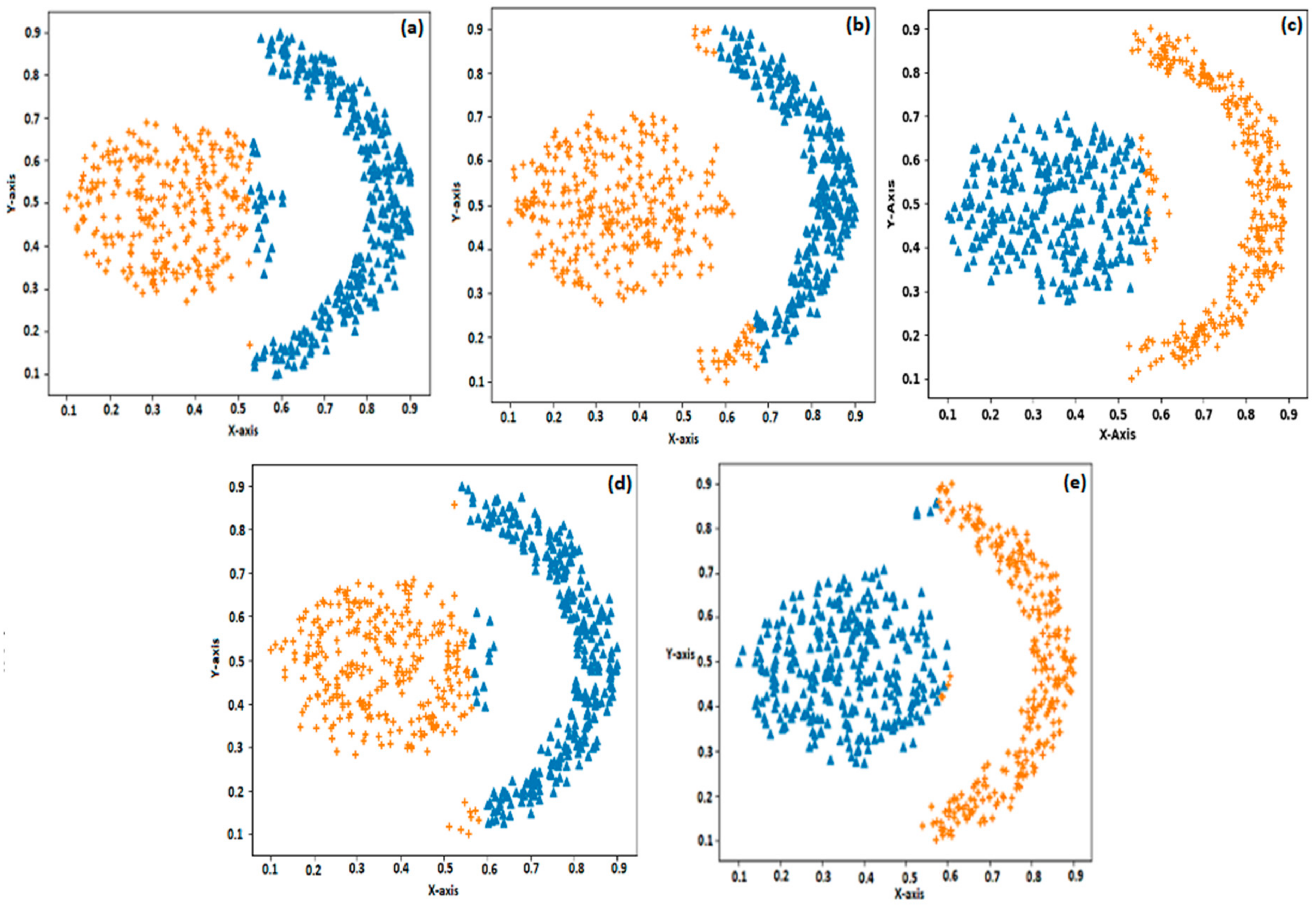
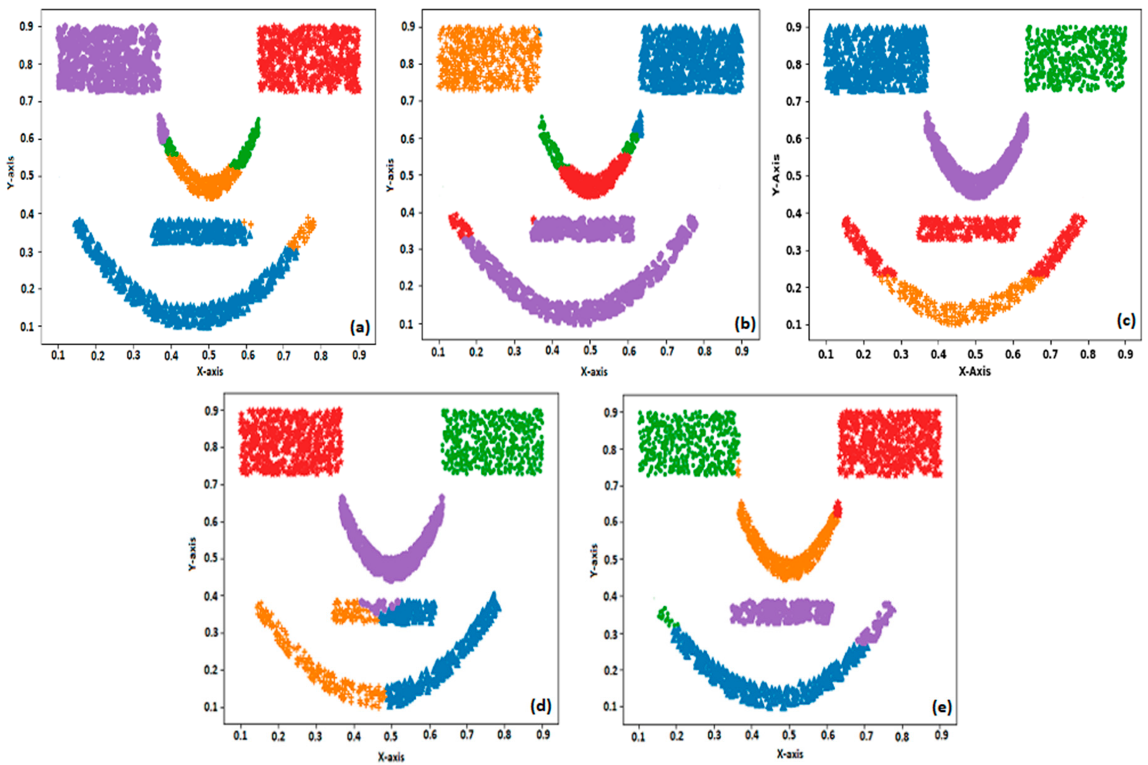
The first synthetic dataset consists of 400 samples and 4 classes in which each class consists of 100 samples and the data distribution is linearly separable. The second dataset consists of 600 samples and 2 classes in which each class consists of 300 samples. The spatial distribution of the second dataset appears as a flame pattern. The third dataset shows the spatial distribution of the face pattern. This dataset consists of 2200 samples and 5 classes with each class consisting of 500, 500, 200, and 500 samples. Here, two classes that form the eyes and nose are linearly separable, whereas the other two parts are nonlinearly separable. The second and third synthetic datasets are more complex to cluster effectively and efficiently.
For each of the synthetic datasets, the BELMKN and other four state-of-the-art clustering methods are applied. The BELMKN uses ELM to perform feature learning with the parameter values set empirically. The feature extracted information from the ELM network is given to BIC as input for cluster prediction. The optimal number of clusters predicted by BIC decides the number of output neurons of the Kohonen Network. The number of hidden neurons is set as 10, 40, and 20, respectively, for the three synthetic datasets. Figure 2 shows that the clustering of the first synthetic dataset using all the clustering methods used in this study resulted in 100% accuracy. This is because all the classes in this dataset are linearly separable. The second dataset (flame pattern) is nonlinearly separable between two classes. We can observe from Figure 3a–e that US-ELM performs better than k-means, SOM, and EM, whereas compared to US-ELM the proposed BELMKN performed better. For the face pattern dataset, the EM algorithm performs better when compared to SOM and k-means as EM algorithm assigns cluster centers probabilistically, whereas k-means and SOM involve crisp-based clustering; the outcome of these clustering methods are shown in Figure 4a–c. Using ELM network, we perform feature learning initially by transforming the data samples in which the assignment of cluster centers become easier for k-means and SOM. It is evident that US-ELM (ELM with k-means) is able to capture nonlinearity well due to ELM-based feature learning but fails to cluster efficiently due to the drawbacks of k-means. In particular, the US-ELM fails to capture the mouth part of face pattern in the dataset, as shown in Figure 4d. This problem is overcome using the proposed BELMKN framework, as shown in Figure 4e.
Overall the proposed BELMKN performs better than all the four methods for the three synthetic datasets. This is due to ELM capturing the nonlinearity in the dataset followed by BIC to predict the number of clusters accurately and finally; the Kohonen network uses competitive learning to cluster the dataset efficiently. Among the conventional methods (k-means, SOM, EM), BELMKN and USELM performed better, which shows the importance of using ELM-based feature learning. Hence, we can use BELMKN for clustering linear, as well as nonlinear, synthetic datasets efficiently.
4. Results and Discussion
In this section, we present the results obtained using BELMKN framework on 10 benchmark datasets from the UCI Database Repository [31,32]. Initially, we describe the characteristics of the dataset, and then we present the results for the number of clusters predicted by BIC with ELM-based feature learning; this is compared to BIC applied on the original dataset. Finally, we compare the clustering performance of BELMKN with other well-known clustering algorithms, namely, k-means [14], SOM [16], EM [33], and USELM [28]. The algorithms were tested on a computer with the Core-i3 processor, 4 GB RAM, Python 2.7, and Windows 10 OS.
4.1. Dataset Description
In the literature, 10 benchmark datasets are widely used to compare the performance of the proposed algorithm. The number of samples, their input dimension, and the number of clusters are shown in Table 1. The BELMKN framework uses three phases on each dataset to extract the clustering accuracy, i.e., ELM for feature learning, and this feature-extracted information is used for cluster prediction using BIC. The feature-extracted information with the predicted number of clusters is given as the input to Kohonen network to compute overall clustering accuracy. The description of the datasets used is as follows:
- Dataset 1:
- The Cancer dataset consists of 2 classes that categorize the tumor as either malignant or benign. It contains 569 samples and 30 attributes.
- Dataset 2:
- The Dermatology dataset is based on the differential diagnosis of erythemato-squamous diseases in dermatology. It consists of 366 samples, 34 attributes, and 6 classes.
- Dataset 3:
- The E. coli dataset is based on the cellular localization sites of proteins. It contains 327 samples, 7 attributes, and 5 classes.
- Dataset 4:
- The Glass dataset is based on the oxide content of each glass type. It contains 214 samples, 9 attributes, and 6 classes.
- Dataset 5:
- The Heart dataset is based on the diagnosis of heart disease. It contains 270 samples, 13 attributes, and 2 classes.
- Dataset 6:
- The Horse dataset is to classify whether the horse will die, survive, or be euthanized. The dataset contains 364 samples, 27 attributes, and 3 classes.
- Dataset 7:
- The Iris dataset is based on the width and length of the sepals and petals of 3 varieties (classes) of flowers, namely, setosa, virginica andversicolor, with 150 samples and 4 attributes.
- Dataset 8:
- The Thyroid dataset is based on whether the thyroid is over-function, normal-function, or under-function (3 classes). The dataset contains 215 samples and 5 attributes.
- Dataset 9:
- The Vehicle dataset is used to classify a vehicle into 4 classes given the silhouette. The dataset contains 846 samples and 18 attributes.
- Dataset 10:
- The Wine dataset is obtained from the chemical analysis of wine obtained from 3 different cultivators (3 classes). The dataset contains 178 samples and 13 attributes.
4.2. Analysis of Cluster Prediction
The Bayesian Information Criterion (BIC) is used to predict the number of clusters for the given dataset. The actual data and the feature extracted data (i.e., by applying ELM) for different datasets are given as input to BIC to predict the number of clusters, as shown in Table 2. In this table, we can observe that there is a difference in the number of clusters predicted by BIC when it is applied directly to the original dataset. The Cancer dataset, using BIC, both with and without ELM-based feature learning, was not able to predict the number of clusters given by the dataset. The ELM-based learning with BIC is not able to predict Heart dataset. This is because ELM is overfitting Cancer and Heart datasets, and, as a result, BIC is not able to capture the number of clusters, whereas in all other cases the prediction is accurate. In case of E. coli, Glass and Horse dataset when BIC applied directly to the original dataset the number of clusters is predicted to be 4, 3, and 2 respectively, instead of 5, 6, and 3. This is because ELM-based feature learning is able to capture the underlying nonlinear distribution of these datasets. Overall, by applying ELM we have carried out a nonlinear feature extraction of the original data, thereby discarding the redundant data that helps BIC to obtain the best partition for the entire data. Hence, prediction accuracy is 80% in the case of ELM-based feature learning with BIC, whereas it is 60% when BIC is applied directly to the dataset. As a result, by using ELM-BIC we are able to obtain the exact number of clusters as given by the dataset.
4.3. Effect of Parameter Settings
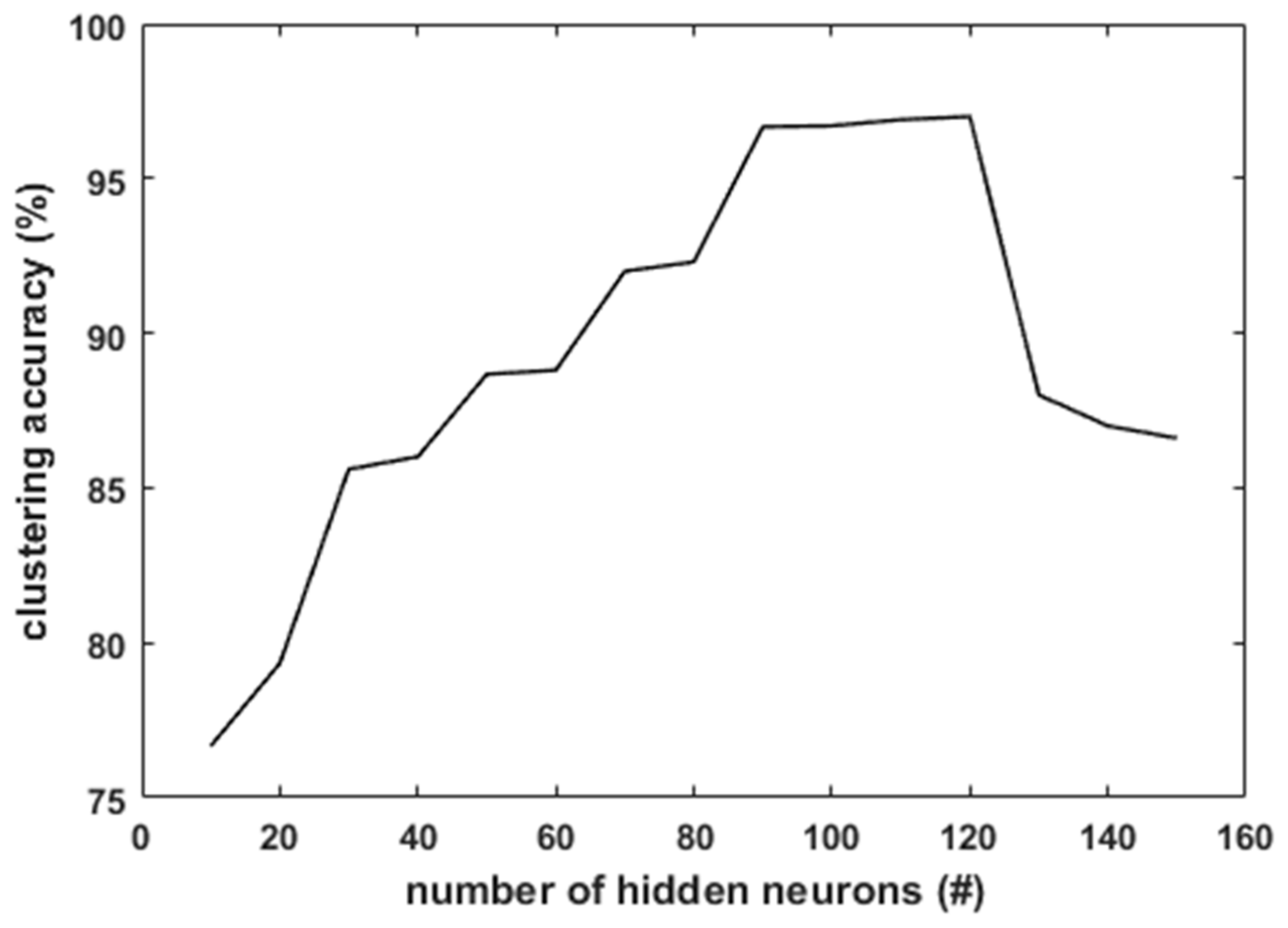
In BELMKN, it is observed that the performance of clustering and convergence rate of the ELM network depends on the number of hidden neurons. ELM requires a sufficient number of hidden neurons to capture the nonlinearity, as it contains only one hidden layer. The number of hidden neurons varied in multiples of 10 from 10 to 150 for each dataset. The variation of the clustering accuracy with the number of hidden neurons for the Iris dataset is shown in Figure 5. It is observed that with 10 hidden neurons, clustering accuracy is less, as class 2 and class 3 samples overlap. This leads to underfitting. Although it is very difficult to determine the exact number of hidden neurons for a given dataset, we can get an approximate estimate by empirically trying different values. It is observed that for Iris Dataset, with 120 hidden neurons, the maximum accuracy is achieved. With further increase in the hidden neurons, the clustering accuracy is observed to decrease due to overfitting. In comparison with the US-ELM [28], in which 97% clustering accuracy was obtained for 1000 hidden neurons, the proposed BELMKN framework uses only 120 hidden neurons to obtain 97% clustering accuracy. Hence, we can observe that BELMKN provides a significant improvement by reducing the number of hidden neurons, which saves computational time.
The other ELM parameter values used are tradeoff parameter , sigma . The parameters and are varied as in the above sequences empirically for each of the 10 datasets. It is observed that with negative orders of magnitude of the hyperparameter , a smoother fit is obtained. On increasing the value of , overfitting is observed. On increasing the value of , which signifies the number of nearest neighbours, overfitting is also observed.
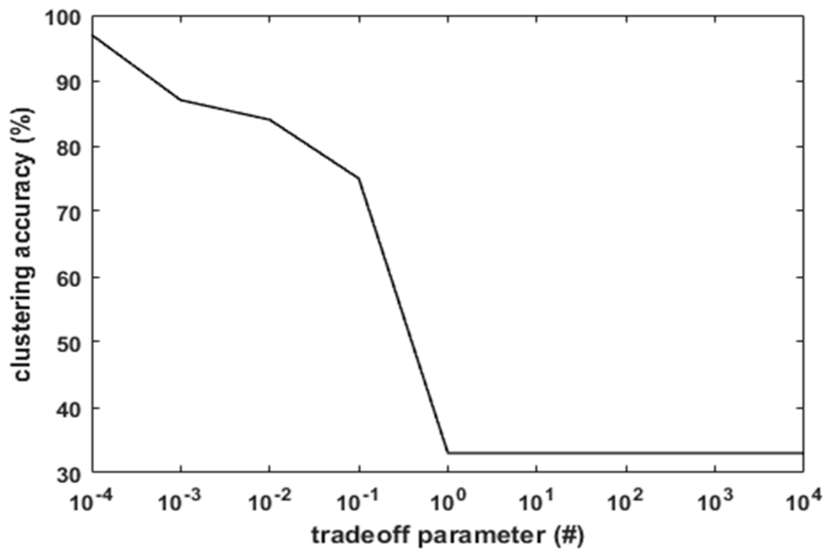
For the Iris dataset, by assigning = 50, the effect of on the clustering accuracy is presented in Figure 6. With , the clustering accuracy is maximum, which is 97%. With , the accuracy is observed to decrease to 85%. On further increase in the value of , the accuracy decreases from 85% to 75%. Hence, it is essential to select the optimal values of the parameters to achieve higher accuracy. Similarly, the parameter setting is done for the remaining datasets.
4.4. Analysis of Clustering Accuracy Using BELMKN
The proposed BELMKN framework is applied to the 10 datasets from UCI repository. The parameters to the ELM network are set empirically as discussed above, and the outputs of the ELM network with BIC cluster prediction are given to the Kohonen network. Hence, the proposed method is a fully automated clustering approach. This automated approach is observed to perform better than the USELM [28] and the traditional clustering approaches such as k-means, SOM, and EM for most of the datasets.
The performance of k-means is observed to be the least for all the datasets. This is because in k-means, the initial centroids are randomly assigned, and cluster centers are iteratively computed. Followed by k-means is SOM, also a linear clustering technique due to the absence of hidden layer. Though k-means and SOM are efficient at grouping linearly separable datasets; SOM overcomes the disadvantage of the k-means approach by using the neighborhood concept, i.e., in SOM the weights of the winning neuron and those neurons within its vicinity (neighborhood threshold) are updated. In Table 3, when we apply k-means and SOM algorithms to Iris dataset, we observe that the class 1 (50 samples), which is linearly separable, is grouped correctly, whereas the grouping of the remaining 100 samples (50 samples of class 2 and 50 samples of class 3) results in more misclassification, as they are nonlinearly separable. Hence, we can observe that k-means and SOM algorithms do not capture the nonlinearity in the dataset. When these algorithms are applied to Glass dataset, it is observed that the overall clustering accuracy is greater but the individual class efficiency is lower, as class 1 and class 2 are dominant in terms of accuracy, with majority of the samples present in these classes (i.e., 70 and 76 samples, respectively), leaving fewer samples to the remaining classes (i.e., class 3, class 4, and class 5 contain 13, 9, and 17 samples, respectively).
The overall accuracy for the k-means in Vehicle dataset seems better; this is due to some of the classes data points tend to dominate, and in some case it is sparse; suppose centers are picked in dominated classes; this results slightly better accuracy. Also, the sparse data points are not fully clustered with better accuracy into the respective classes. Overall, it is observed that the accuracy reduces when the sparse data points are overlapped on the dominated data points. From Table 3, we can also observe that the EM algorithm performs better than k-means and SOM. EM clustering is performed probabilistically, unlike k-means and SOM, which use the crisp assignment of the samples to the clusters. When compared to k-means, SOM, and EM algorithms, USELM performs better. In USELM, ELM performs non-linear feature learning, and the extracted features are given to k-means for clustering [28]. In USELM, there is no automatic prediction of the number of clusters [3]; it also suffers from the drawbacks of k-means. In the proposed BELMKN framework, non-linearity is captured well, similarly to USELM network, but the problem of cluster prediction is overcome and the clustering accuracy is improved by using Kohonen Network as the partitional clustering algorithm. Overall, it is observed that the proposed BELMKN framework performs the best among all the clustering techniques used in this study.
In Table 4, the average clustering accuracy for all the clustering techniques with 10 datasets is shown. In this table, we observe that BELMKN has the highest average clustering accuracy, followed by US-ELM. Among traditional clustering methods, EM is better than k-means, and SOM is better than the k-means algorithm. In Table 5, the sum of the ranks for all the datasets taken from Table 3 for each of the clustering techniques is presented. By ranking the sum of ranks, the proposed BELMKN is better than all other clustering methods. This is followed by USELM, whereas EM is better than SOM and k-means, and SOM is better than k-means.
5. Conclusions
This paper presents the Bayesian Extreme Learning Machine Kohonen Network (BELMKN) framework, which consists of three levels, to improve the clustering accuracy of the nonlinearly distributed dataset. ELM is used for feature learning, followed by BIC a model selection technique to extract the optimal number of clusters and the Kohonen Network for clustering the dataset. It is also observed that the performance of the BELMKN network depends on the number of parameters such as the tradeoff parameter (), the number of nearest neighbours (), and the number of hidden neurons (), which have to be set empirically for each dataset. These parameters need to be fine-tuned to avoid overfitting or underfitting.
The clustering task is successfully accomplished by applying 10 benchmark datasets from the UCI machine learning repository using the process of partitional clustering using the BELMKN. The clustering performance is compared with k-means, Self-Organizing Maps, the EM Algorithm, and USELM. From the results obtained, we can conclude that BELMKN is reliable and involves efficient clustering in terms of accuracy, which can also be used on complex datasets.
Although the results are very promising, there is still room for improvement. For example, it is challenging to generate optimal cluster centers with a big dataset with a varying number of dimensions (i.e., some class data points may have fewer samples in comparison with others); this may provide opportunities for further research. In addition, the clustering of the big dataset by implementing the BELMKN as a hierarchical clustering may provide better clustering efficiency. It will be useful to investigate these topics further.
Author Contributions
J.S. conceived and designed the research; S.S.C., N.G., J.S., and M.T. developed and analyzed the data; S.S.C., N.G., J.S., M.T., and I.M. wrote and edited the paper.
Conflicts of Interest
The authors declare no conflict of interest.
References
- Jain, A.K.; Murty, M.N.; Flynn, P.J. Data clustering: A review. ACM Comput. Surv. 1999, 31, 264–323. [Google Scholar] [CrossRef]
- Senthilnath, J.; Deepak, K.; Benediktsson, J.A.; Xiaoyang, Z. A Novel Hierarchical Clustering Technique Based on Splitting and Merging. Int. J. Image Data Fusion 2016, 7, 19–41. [Google Scholar] [CrossRef]
- Google Scholar. Available online: http://scholar.google.com (accessed on 28 March 2018).
- Jain, A.K. Data clustering: 50 years beyond K-means. Pattern Recognit. Lett. 2010, 31, 651–666. [Google Scholar] [CrossRef]
- Yang, X.; Lo, C.P. Using a time series of satellite imagery to detect land use and land cover changes in the Atlanta, Georgia metropolitan area. Int. J. Remote Sens. 2002, 23, 1775–1798. [Google Scholar] [CrossRef]
- Senthilnath, J.; Omkar, S.N.; Mani, V.; Tejovanth, N.; Diwakar, P.G.; Shenoy, A.B. Hierarchical clustering algorithm for land cover mapping using satellite images. IEEE J. Sel. Top. Appl. Earth Obs. Remote Sens. 2012, 5, 762–768. [Google Scholar] [CrossRef]
- Gvishiani, A.D.; Dzeboev, B.A.; Agayan, S.M. A New Approach to Recognition of the Strong Earthquake ProneAreas in the Caucasus. Izv. Phys. Solid Earth 2013, 49, 747–766. [Google Scholar] [CrossRef]
- Rui, X.; Donald, C.W. Clustering Algorithms in Biomedical Research—A Review. IEEE Rev. Biomed. Eng. 2010, 3, 120–154. [Google Scholar]
- Silhavy, R.; Silhavy, P.; Prokopova, Z. Evaluating Subset Selection Methods for Use Case Points Estimation. Inf. Softw. Technol. 2018, 97, 1–9. [Google Scholar] [CrossRef]
- Raghu, K.; James, M.K. A Possibilistic Approach to Clustering. IEEE Trans. Fuzzy Syst. 1993, 1, 98–110. [Google Scholar]
- Ron, Z.; Amnon, S. A Unifying Approach to Hard and Probabilistic Clustering. In Proceedings of the 10th IEEE International Conference on Computer Vision, Beijing, China, 7–21 October 2005; pp. 294–301. [Google Scholar]
- Sueli, A.M.; Joab, O.L. Comparing SOM neural network with Fuzzy c-means, K-means and traditional hierarchical clustering algorithms. Eur. J. Oper. Res. 2006, 174, 1742–1759. [Google Scholar]
- Rui, X.; Donald, W. Survey of Clustering Algorithms. IEEE Trans. Neural Netw. 2005, 16, 645–678. [Google Scholar]
- Tapas, K.; David, M.M.; Nathan, S.N.; Christine, D.P.; Ruth, S.; Angela, Y.W. An efficient k-means clustering algorithm: Analysis and implementation. IEEE Trans. Pattern Anal. Mach. Intell. 2002, 24, 881–892. [Google Scholar]
- Jean-Claude, F.; Patrick, L.; Marie, C. Advantages and drawbacks of the Batch Kohonen algorithm. In Proceedings of the 10th Eurorean Symposium on Artificial Neural Networks, Bruges, Belgium, 24–26 April 2002; pp. 223–230. [Google Scholar]
- Paul, M.; Shaw, K.C.; David, W. A Comparison of SOM Neural Network and Heirarchical Clustering Methods. Eur. J. Oper. Res. 1996, 93, 402–417. [Google Scholar]
- Senthilnath, J.; Dokania, A.; Kandukuri, M.; Ramesh, K.N.; Anand, G.; Omkar, S.N. Detection of tomatoes using spectral-spatial methods in remotely sensed RGB images captured by UAV. Biosyst. Eng. 2016, 146, 16–32. [Google Scholar] [CrossRef]
- Dempster, A.P.; Laird, N.M.; Rubin, D.B. Maximum Likelihood from Incomplete Data via the EM Algorithm. J. R. Stat. Soc. Ser. B 1977, 39, 1–38. [Google Scholar]
- Li, H.; Zhang, K.; Jiang, T. The regularized EM algorithm. In Proceedings of the 20th International Conference on Artificial Intelligence, Pittsburgh, PA, USA, 9–13 July 2005; pp. 807–812. [Google Scholar]
- Senthilnath, J.; Manasa, K.; Akanksha, D.; Ramesh, K.N. Application of UAV imaging platform for vegetation analysis based on spectral-spatial methods. Comput. Electron. Agric. 2017, 140, 8–24. [Google Scholar] [CrossRef]
- Senthilnath, J.; Kulkarni, S.; Raghuram, D.R.; Sudhindra, M.; Omkar, S.N.; Das, V.; Mani, V. A novel harmony search-based approach for clustering problems. Int. J. Swarm Intell. 2016, 2, 66–86. [Google Scholar] [CrossRef]
- Ding, S.; Zhang, N.; Zhang, J.; Xu, X.; Shi, Z. Unsupervised extreme learning machine with representational features. Int. J. Mach. Learn. Cybern. 2017, 8, 587–595. [Google Scholar] [CrossRef]
- Akogul, S.; Erisoglu, M. An Approach for Determining the Number of Clusters in a Model-Based Cluster Analysis. Entropy 2017, 19, 452. [Google Scholar] [CrossRef]
- Burnham, K.P.; Anderson, D.R. Multimodel inference: Understanding AIC and BIC in model selection. Sociol. Methods Res. 2004, 33, 261–304. [Google Scholar] [CrossRef]
- Huang, G.; Huang, G.B.; Song, S.; You, K. Trends in extreme learning machines: A review. Neural Netw. 2015, 61, 32–48. [Google Scholar] [CrossRef] [PubMed]
- Khan, B.; Wang, Z.; Han, F.; Iqbal, A.; Masood, R.J. Fabric Weave Pattern and Yarn Color Recognition and Classification Using a Deep ELM Network. Algorithms 2017, 10, 117. [Google Scholar] [CrossRef]
- Huang, G.B.; Zhou, H.; Ding, X.; Zhang, R. Extreme learning machine for regression and multiclass classification. IEEE Trans. Syst. Man Cybern. B 2012, 42, 513–529. [Google Scholar] [CrossRef] [PubMed]
- Huang, G.; Song, S.; Gupta, J.N.; Wu, C. Semi-supervised and unsupervised extreme learning machines. IEEE Trans. Cybern. 2014, 44, 2405–2417. [Google Scholar] [CrossRef] [PubMed]
- Schwarz, G. Estimating the dimension of a model. Ann. Stat. 1978, 6, 461–464. [Google Scholar] [CrossRef]
- Huang, Z.; Ng, M.K. A fuzzy k-modes algorithm for clustering categorical data. IEEE Trans. Fuzzy Syst. 1999, 7, 446–452. [Google Scholar] [CrossRef] [Green Version]
- Blake, C.L.; Merz, C.J. Repository of Machine Learning Databases; Department of Information and Computer Science, University of California: Irvine, CA, USA, 1998. [Google Scholar]
- Senthilnath, J.; Omkar, S.N.; Mani, V. Clustering using firefly algorithm: Performance study. Swarm Evolut. Comput. 2011, 1, 164–171. [Google Scholar] [CrossRef]
- Bhola, R.; Krishna, N.H.; Ramesh, K.N.; Senthilnath, J.; Anand, G. Detection of the power lines in UAV remote sensed images using spectral-spatial methods. J. Environ. Manag. 2018, 206, 1233–1242. [Google Scholar] [CrossRef] [PubMed]
Figure 1.
BELMKN architecture.
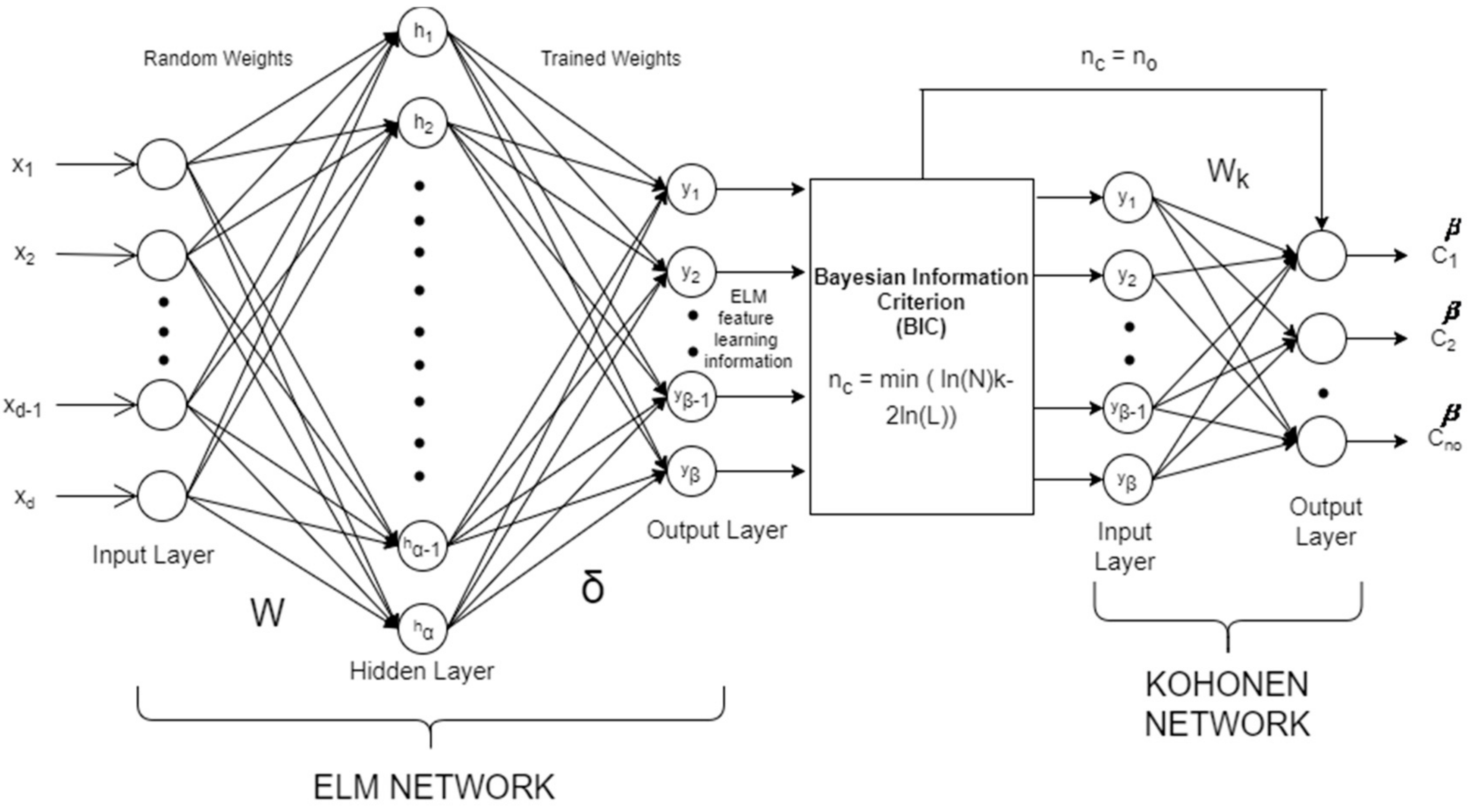
Figure 2.
Four-class, linearly separable distribution.
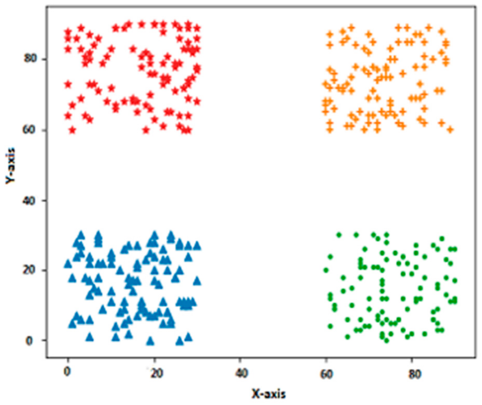
Figure 3.
Clustering of flame pattern distribution using (a) k-means; (b) SOM; (c) EM; (d) US-ELM; and (e) BELMKN.
Figure 3.
Clustering of flame pattern distribution using (a) k-means; (b) SOM; (c) EM; (d) US-ELM; and (e) BELMKN.

Figure 4.
Clustering of face pattern distribution using (a) k-means; (b) SOM; (c) EM; (d) US-ELM; and (e) BELMKN.
Figure 4.
Clustering of face pattern distribution using (a) k-means; (b) SOM; (c) EM; (d) US-ELM; and (e) BELMKN.

Figure 5.
Clustering accuracy versus number of hidden neurons.

Figure 6.
Clustering accuracy versus tradeoff parameter .


Table 1.
Properties of the dataset.
| Sl. No. | Dataset | Number of Samples | Input Dimension | Number of Clusters |
|---|---|---|---|---|
| 1 | Cancer | 569 | 30 | 2 |
| 2 | Dermatology | 366 | 34 | 6 |
| 3 | E. coli | 327 | 7 | 5 |
| 4 | Glass | 214 | 9 | 6 |
| 5 | Heart | 270 | 13 | 2 |
| 6 | Horse | 364 | 27 | 3 |
| 7 | Iris | 150 | 4 | 3 |
| 8 | Thyroid | 215 | 5 | 3 |
| 9 | Vehicle | 846 | 18 | 4 |
| 10 | Wine | 178 | 13 | 3 |
Table 2.
Cluster predicted using BIC for actual data and ELM-based feature learning data.
| Dataset | Cancer | Dermatology | E. coli | Glass | Heart | Horse | Iris | Thyroid | Vehicle | Wine |
|---|---|---|---|---|---|---|---|---|---|---|
| Actual Clusters | 2 | 6 | 5 | 6 | 2 | 3 | 3 | 3 | 4 | 3 |
| BIC cluster predicted on original dataset | 3 | 6 | 4 | 3 | 2 | 2 | 3 | 3 | 4 | 3 |
| BIC cluster predicted using ELM | 3 | 6 | 5 | 6 | 3 | 3 | 3 | 3 | 4 | 3 |
Table 3.
Clustering accuracy percentage and ranking of various techniques on each dataset.
| Sl No. | Dataset | k-Means | SOM | EM | USELM | BELMKN |
|---|---|---|---|---|---|---|
| 1 | Cancer | 85.4% (5) | 86% (4) | 91.21% (2) | 90% (3) | 92.6% (1) |
| 2 | Dermatology | 26.2% (5) | 32% (4) | 67.75% (3) | 82% (2) | 90.1% (1) |
| 3 | E. coli | 59.9% (4) | 61% (3) | 77.98% (2) | 82% (1) | 82% (1) |
| 4 | Glass | 54.2% (1) | 54% (2) | 47.66% (4) | 42% (5) | 48% (3) |
| 5 | Heart | 59.2% (4) | 60% (3) | 53.33% (5) | 70% (2) | 75.5% (1) |
| 6 | Horse | 48% (3) | 48% (3) | 43.4% (4) | 65% (1) | 63.18% (2) |
| 7 | Iris | 80% (5) | 82% (4) | 90% (3) | 96% (2) | 97% (1) |
| 8 | Thyroid | 86% (5) | 87% (4) | 94.27% (3) | 89% (3) | 90.5% (2) |
| 9 | Vehicle | 44% (2) | 44% (2) | 45.035% (1) | 42% (3) | 41% (4) |
| 10 | Wine | 70% (5) | 75% (4) | 90.44% (3) | 94% (2) | 96.6% (1) |
Table 4.
Average clustering accuracy and general ranking of the techniques of all datasets.
| Clustering Algorithm | k-Means | SOM | EM | USELM | BELMKN |
|---|---|---|---|---|---|
| Average | 61.29 | 62.9 | 70.1 | 75.2 | 77.65 |
| Rank | 5 | 4 | 3 | 2 | 1 |
Table 5.
The sum of ranking of the techniques and general ranking based on total ranking.
| Clustering Algorithm | k-Means | SOM | EM | USELM | BELMKN |
|---|---|---|---|---|---|
| Total | 39 | 33 | 30 | 24 | 17 |
| Rank | 5 | 4 | 3 | 2 | 1 |
© 2018 by the authors. Licensee MDPI, Basel, Switzerland. This article is an open access article distributed under the terms and conditions of the Creative Commons Attribution (CC BY) license (http://creativecommons.org/licenses/by/4.0/).
Share and Cite
MDPI and ACS Style
Senthilnath, J.; Simha C, S.; G, N.; Thapa, M.; M, I. BELMKN: Bayesian Extreme Learning Machines Kohonen Network. Algorithms 2018, 11, 56. https://doi.org/10.3390/a11050056
AMA Style
Senthilnath J, Simha C S, G N, Thapa M, M I. BELMKN: Bayesian Extreme Learning Machines Kohonen Network. Algorithms. 2018; 11(5):56. https://doi.org/10.3390/a11050056
Chicago/Turabian StyleSenthilnath, J., Sumanth Simha C, Nagaraj G, Meenakumari Thapa, and Indiramma M. 2018. "BELMKN: Bayesian Extreme Learning Machines Kohonen Network" Algorithms 11, no. 5: 56. https://doi.org/10.3390/a11050056
Note that from the first issue of 2016, this journal uses article numbers instead of page numbers. See further details here.